
Submitted:
29 May 2025
Posted:
30 May 2025
You are already at the latest version
Abstract
Estimating sparse solutions in penalized tensor models poses a significant meth- odological challenge in high-dimensional settings. Although methods such as the Cenet- Tucker model incorporate Elastic Net penalties to achieve sparse and orthogonal repre- sentations, their stability under minimal perturbations remains a critical issue. This article proposes a bootstrap-based extension to stabilize the selected support, formulating a com- prehensive protocol for resampling, model fitting, and evaluation, applicable to penalized tensor models. Stability metrics are introduced, a rigorous simulation study is conducted, and the GSparseBoot package is being actively developed in R as a reproducible and mod- ular computational tool. Although still under development, GSparseBoot already shows promising performance and reflects a strong commitment to accessible, open-source im- plementation of advanced statistical methods. In simulations, the use of calibrated boot- strap increased the Stable Selection Index (SSI) by over 25%, reduced the standard devia- tion of the support by 40%, and improved the average Jaccard Index across replicates— demonstrating a substantial enhancement in the structural consistency of the model. This article presents a well-founded methodological contribution, empirically validated and aligned with modern standards of reproducibility in data science.
Keywords:
tensor
; elastic net
; penalization
; stability
; selection metrics
1. Introduction
The stability of selection models in high-dimensional settings has become a growing topic of concern in modern statistics. Penalized tensor decomposition models—such as the CenetTucker—have gained attention for their ability to model complex data structures, including neuroimaging, transcriptomics, or functional connectivity matrices, while preserving the intrinsic multidimensional organization of the data (Kolda & Bader, 2009; Sidiropoulos et al., 2017). However, the introduction of LASSO (Tibshirani, 1996) and Elastic Net (Zou et al., 2006) penalties, though useful in inducing sparsity, does not ensure stability in variable selection (Bühlmann & van de Geer, 2011).
This instability has been well documented in the context of generalized linear models (Lim & Yu, 2016; Meinshausen & Bühlmann, 2010), yet its analysis in tensor-based frameworks remains underexplored. The problem is methodologically profound: small perturbations in the sample can lead to substantial variations in the selected factors, thereby compromising the statistical reproducibility and scientific validity of the inferences (Yu et al., 2019).
In this context, bootstrap—originally introduced by Efron (1979) as a tool for evaluating variability and uncertainty—emerges as a viable alternative for estimating the stability of sparse supports. In penalized regression, bootstrap variants have proven effective in assessing variable selection performance (Bach, 2008; Shah & Samworth, 2013), and their adaptation to tensor models constitutes a novel methodological contribution. Despite its potential, the systematic application of bootstrap to three-way sparse solutions remains in its infancy.
This article proposes both a classic and adjusted bootstrap protocol, specifically designed for the CenetTucker model (González-García, 2019), to quantify and improve the stability of sparse supports. Unlike Stability Selection (Meinshausen & Bühlmann, 2010), the proposed approach naturally aligns with the tensor structure and yields directly interpretable metrics on the selected elements. Through controlled simulations and the development of a computational solution in R (the GSparseBoot package), we demonstrate the efficacy of the approach in enhancing the structural consistency of sparse solutions.
The following sections present the formalization of the penalized model, the design of the bootstrap protocol, the definition of stability metrics, the computational implementation, and a simulation study with quantitative validation. The article concludes with a discussion of the methodological implications and future extensions, including Bayesian bootstrap and non-convex penalties.
2. Methodological Foundations
2.1. From the Tucker Model to the CenetTucker
The Tucker decomposition (Tucker, 1966) is a generalization of Principal Component Analysis (PCA) to higher-order data structures—i.e., tensors. Let be a three-dimensional tensor representing data structured across three modes—for instance, subject variable condition. The Tucker decomposition seeks a low-dimensional representation that preserves the original multiway structure. This representation is formally expressed as:
where: is the core tensor, , , are the factor (or loading) matrices, and denotes the mode-n product between a tensor and a matrix (Kolda & Bader, 2009).
This decomposition allows latent interactions between dimensions to be represented without losing the original array structure (Kolda & Bader, 2009). The model is estimated by solving the following optimization problem:
This problem minimizes the squared reconstruction loss without imposing any structural constraints on the factors. Although this formulation is effective for capturing latent components, it suffers from critical limitations when applied in high-dimensional contexts. The loading matrices tend to be dense, making interpretation difficult and preventing explicit variable selection (Zhou et al., 2013). Moreover, the model exerts no control over the magnitude of the estimated coefficients, which can amplify overfitting in response to minor perturbations (Hastie, Tibshirani, & Friedman, 2009). This lack of regularization also makes it sensitive to collinearity among dimensions, undermining the stability and reproducibility of the results (Meinshausen & Bühlmann, 2010).
Schematic representation of the Tucker model (Figure 1).
The three-dimensional tensor is decomposed into a core tensor and factor matrices , each associated with a specific mode of the tensor. This factorization is constructed through sequential mode-wise matrix products, typically based on singular value decomposition.
However, in high-dimensional settings or under low signal-to-noise ratios, this approach may yield dense, numerically unstable, and poorly interpretable solutions. To address these shortcomings, the CenetTucker, proposed by González-García (2019), introduces an Elastic Net penalty on the factor matrices .
Formalization of the CenetTucker Model
The CenetTucker proposal modifies the previous optimization problem by incorporating two penalty terms on each loading matrix, combining: the norm, which induces sparsity by shrinking some coefficients exactly to zero (Tibshirani, 1996), and the -norm, which stabilizes the estimates by discouraging excessively large coefficients (Zou & Hastie, 2005).
The objective function of the CenetTucker model is expressed as:
where regulates the intensity of the sparsity penalty, and controls the penalty on coefficient magnitudes. This formulation extends the regularization framework of the Elastic Net to tensor structures, enabling more stable and parsimonious estimations.
The inclusion of the - term forces solutions toward the vertices of the feasible set, promoting sparse estimators, while the -penalty acts as a shrinkage operator that reduces variance. The resulting model thus achieves a balance between parsimony, numerical stability, and multilateral representational capacity—desirable properties in high-dimensional problems with complex latent structures (Zou & Hastie, 2005; Bühlmann & van de Geer, 2011).
Schematic representation of the CenetTucker model (Figure 2).
The tensor is approximated by a core tensor and penalized loading matrices , obtained through Elastic Net regularization. The blank areas symbolize zero coefficients, reflecting the sparsity induced by the -penalty, while the non-zero coefficients are controlled by the penalty.
In summary, the Tucker model seeks the best reconstruction of the tensor without imposing additional constraints, which may result in dense and unstable solutions. In contrast, the CenetTucker model modifies the loss function by adding regularization terms that yield sparser, more interpretable, and robust representations. This step is essential as a prelude to the development of stability evaluation mechanisms based on resampling techniques such as the bootstrap, which will be introduced in the following sections.
The contrast is notable between the Tucker-based estimation on the left (dense matrices) and the CenetTucker-based estimation on the right (sparse matrices with many zeros) (Figure 3). The Elastic Net penalty enforces sparsity and magnitude control on the loading matrices, resulting in more interpretable and robust solutions.
2.2. Bootstrap: Fundamentals, Variants, and Application to Penalized Models
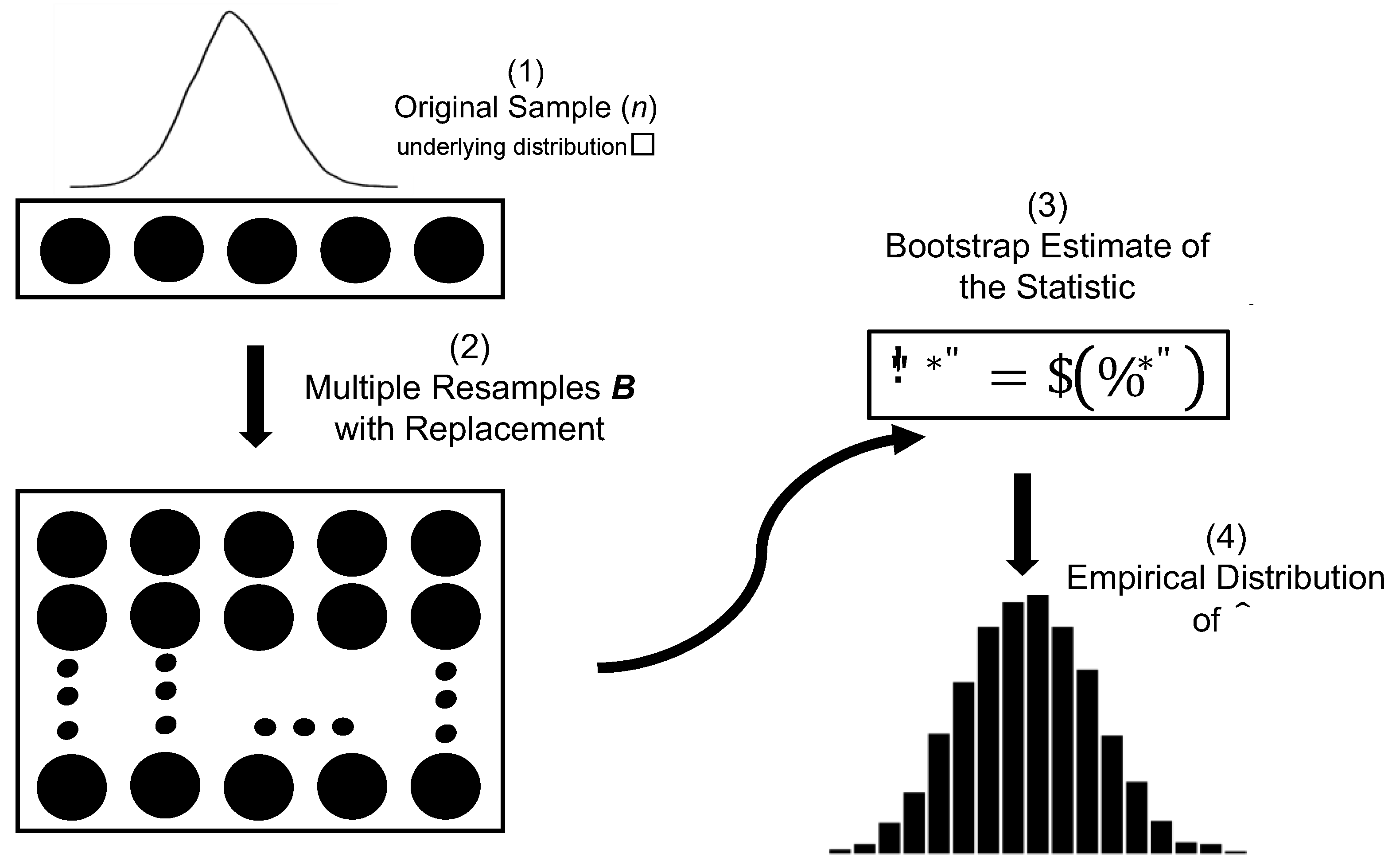
The bootstrap method, introduced by Efron (1979), represents one of the most influential contributions of modern statistics. Its fundamental principle lies in estimating the empirical distribution of an estimator through resampling with replacement from the original sample, thereby avoiding strong parametric assumptions about the population.
From a mathematical standpoint, the bootstrap method aims to estimate the distribution of an estimator without requiring information about the underlying distribution . Suppose we have a sample drawn i.i.d. from an unknown population , and we wish to estimate a functional , such as the mean, median, or a regression coefficient. Since is not observable, it is replaced by the empirical distribution which assigns a mass of to each observation.
The classical bootstrap procedure is structured as shown in Table 1.
The generality of this method has made it a fundamental tool in linear models, regression, classification, survival analysis, and time series modeling (Davison & Hinkley, 1997; Efron & Tibshirani, 1993). Its robustness is particularly useful when asymptotic distributions are either unavailable or unreliable due to the complexity of the estimator.
Figure 4.
Bootstrap Graphic Representation.
2.2.1. Bootstrap in High Dimensionality and Penalization
In penalized models such as LASSO (Tibshirani, 1996) or Elastic Net (Zou & Hastie, 2005), the focus of the bootstrap has shifted from point estimation to the assessment of support stability. This perspective is especially relevant in the presence of structural sparsity. The support of an estimator denoted as:
is the set of variables selected by the model—that is, those with non-zero coefficients. In sparse models, this set directly defines the structural interpretation of the model. Its variability in response to small changes in the data reveals the sensitivity of the selection procedure.
Bach (2008) introduced the concept of Bolasso, a combination of bootstrap and Lasso, and showed that the estimated support can vary significantly across bootstrap replicates, especially under collinearity or high variance. Formally, if is the bootstrap sample, and the corresponding penalized solution, then:
para muchos pares .
This variability reveals that penalization does not always guarantee stability, especially in the presence of noise or internal correlations among predictors.
In response, Shah and Samworth (2013) proposed the Stability Selection technique, which introduces thresholding rules on the inclusion frequency of each variable across bootstrap replicates:
where represents the proportion of times that variable is selected. The final selected set is then defined as:
where is a stability threshold. This approach enables the control of the Per-Family Error Rate (PFER) under certain conditions, transforming the bootstrap into a tool for structural validation, beyond its original role as an inferential technique.
Shah and Samworth (2013) demonstrated that if two key parameters are controlled:
- the expected number of variables selected by each penalized model (e.g., by fixing an upper bound),
- : a sufficiently high stability threshold (e.g., 0.8),
then, under the assumption of independence among irrelevant variables, it is possible to guarantee that:
where denotes the maximum selection probability of an irrelevant variable (typically assumed to be very low or negligible).
This result establishes, for the first time in this class of procedures, an explicit upper bound on the expected number of false positives —the so-called Per-Family Error Rate (PFER)— without requiring strong assumptions about the estimator’s distribution or the use of multiple testing corrections.
In the framework proposed by Shah and Samworth (2013), the inclusion frequency of each variable is estimated empirically via bootstrap replicates, and a selection threshold is applied to construct a final support set with statistical control properties. This mechanism elevates bootstrap from a purely inferential tool to a structural validation instrument, complementing the penalized model’s decisions with guarantees of stability.
The strategy has proven particularly useful in high-dimensional settings, where collinearity and overfitting can compromise the reproducibility of sparse models (Meinshausen & Bühlmann, 2010; Shah & Samworth, 2013; Bach, 2008).
2.2.2. Bootstrap Applied to CenetTucker
A bootstrap resampling protocol specifically adapted to the CenetTucker model is proposed, with the aim of assessing and improving the stability of the sparse support in each mode of the tensor, while preserving the multiway architecture and enabling the estimation of mode-specific metrics. Unlike traditional approaches developed in vector or matrix settings, this implementation maintains the structural dependencies across modes, allowing for a rigorous evaluation of the penalized model’s structural robustness.
Let be a third-order tensor. The resampling procedure is performed over mode-1, corresponding to the observational units, generating bootstrap replicates ), defined as:
This scheme ensures that the internal correlations between modes 2 and 3 (variables and conditions) remain intact across all replicates, preserving structural coherence and avoiding biases induced by resampling schemes incompatible with the tensor’s multiway structure. Therefore, this resampling design constitutes the foundation for structural stability assessment mode by mode, allowing for a precise quantification of the robustness of the penalized support obtained via CenetTucker.
Once the bootstrap replicates are generated, the penalized model is fitted on each of them, estimating in every case the sparse loading matrix and extracting the corresponding support.
2.2.3. Penalized Fitting and Support Extraction in Bootstrap Replicates
For each bootstrap replicate , generated by resampling along mode-1 of the original tensor, the CenetTucker model is fitted by solving the following optimization problem:
This model penalizes the mode-specific loading matrices , , using a combination of the , norm, which induces sparsity by shrinking coefficients to zero (Tibshirani, 1996), and the norm, which stabilizes estimates by shrinking the magnitude of the coefficients (Zou and Hastie, 2005).
The Elastic Net penalty provides a balance between interpretability (through sparse solutions) and numerical stability, which is essential in high-dimensional contexts.
2.2.4. Support Extraction in Each Bootstrap Replicate
Once the model is fitted on each replicate , the penalized support is extracted for each mode. It is defined as the set of active rows—that is, those containing at least one non-zero coefficient—in the corresponding loading matrices. A reconstructed estimate of the original tensor is obtained, formally:
where , , are the estimated loading matrices from bootstrap replicate , and is the corresponding core tensor. These penalized matrices reflect the latent structure detected by the model, filtered by the regularization effects imposed by the Elastic Net penalty.
The penalized support in each mode is defined as the set of active rows, that is, those with at least one non-zero entry in the respective loading matrix. Formally:
These definitions are based on the norm, which counts the number of non-zero elements in each row. This criterion aligns with the geometric interpretation of sparsity: a row with all zero coefficients indicates that the corresponding unit (observation, variable, or condition) does not contribute to the latent structure of the estimated tensor.
From the bootstrap replicates, three collections of supports are obtained—one for each tensor mode:
These collections constitute the foundation for the mode-wise structural stability quantification developed in the previous section.
2.2.5. Justification of Variability Across Replicates
The variation observed in the supports obtained from the BBB bootstrap replicates can be interpreted as an empirical manifestation of the inherent instability of the model in the presence of high dimensionality, collinearity, or a low signal-to-noise ratio. This instability is formalized through the lack of support agreement across replicates:
where represents any row of , or , depending on the mode considered. This variability suggests that the model, although sparse, is not necessarily stable, and that the support can fluctuate significantly as a function of the resampling.
Such an observation justifies the introduction of aggregated metrics—such as inclusion frequency, the Jaccard index, or the Stable Selection Index (SSI)—which allow for an explicit quantification and reporting of the model’s structural stability, thereby providing objective criteria for reproducible interpretation of the penalized support.
In this context, no formal demonstration of asymptotic properties is required, since stability is evaluated empirically through the behavior of the sparse support under resampling. This approach follows the methodology adopted by Bach (2008) and Shah & Samworth (2013), where structural validation is performed through replicability rather than theoretical guarantees.
- Structural Stability Metrics by Mode
2.3. Inclusion Frequency
The first metric proposed to assess the structural stability of the penalized model is the inclusion frequency, which empirically estimates the probability that each row of the loading matrices is selected as part of the sparse support in the resampling process. The use of inclusion frequency as an empirical stability metric has been widely promoted within the framework of Stability Selection (Meinshausen & Bühlmann, 2010; Shah & Samworth, 2013), as well as in bootstrap-based variants such as Bolasso (Bach, 2008).
Let be the number of bootstrap replicates generated and let be the estimated support for mode-1 in replicate , that is, the set of active rows in . Then, the inclusion frequency for index is defined as:
where is the indicator function. This metric counts how many times row iii has been selected across the replicates, and it is interpreted as an empirical estimate of its structural relevance.
The inclusion frequency is analogously defined for modes 2 and 3:
These frequencies allow the identification of those units, variables, or conditions that are consistently selected by the penalized model, serving as a key indicator of structural stability.
What does Figure 5 represent?
Each bar indicates the inclusion frequency of a row in the penalized support across bootstrap replicates. Specifically, the height of each bar represents:
This is interpreted as an empirical probability of selection, reflecting how stable or consistent the inclusion of that row is in the penalized model. Values close to 1 indicate high stability; values close to 0 indicate high instability.
Inclusion frequency supports several forms of quantitative interpretation:
(i) Overall average frequency: Estimates the mean level of inclusion per mode:
.
(ii) Proportion of rows with high or low inclusion: Quantifies how many rows have (high stability) or (high instability), to assess structural concentration or dispersion.
(iii) Dispersion of frequencies (variance): Can be computed as:
which indicates how homogeneous or dispersed the selection is within each mode.
(iv) Comparison across modes: By analyzing the frequency patterns in each mode, one can identify where the penalized model exhibits greater stability. For instance, if mode shows a higher concentration of values near 1 compared to or , this suggests that the latent structure in that mode is more robust or less sensitive to resampling.
Based on these definitions, Figure 5 can be interpreted as follows: there is considerable variability in inclusion frequencies across the different modes. In mode , approximately 40% of the rows exhibit frequencies above 0.8, indicating notable structural stability in the support. In contrast, in mode , less than 20% of the rows reach that threshold, suggesting lower structural consistency in that dimension.
This contrast highlights that the penalized model identifies more robust latent patterns in mode A, whereas in mode , selection is more sensitive to resampling. This sensitivity may be associated with collinearity or weak signal along that axis of the tensor.
2.4. Average Jaccard Index
The Jaccard index is a classical measure of similarity between sets and is particularly useful in the context of penalized models with resampling, where the goal is to evaluate the structural consistency of the estimated support across different replicates. Originally formulated by Jaccard (1901), this metric has been widely adopted in statistical learning contexts to assess the stability of variable selection (Meinshausen & Bühlmann, 2010; Shah & Samworth, 2013).
In particular, its application to sparse support analysis allows for the identification of coherent or inconsistent structural configurations across multiple bootstrap replicates.
Given a collection of bootstrap replicates, the Jaccard index between two replicates and is defined as:
where and are the sets of indices selected as support in bootstrap replicate and , respectively.
The average Jaccard index for a given mode (for example, mode-1) is computed by considering all pairwise combinations of replicates:
The average Jaccard index reflects the overall coherence of the support estimated by the penalized model. Values close to 1 indicate that the sets selected across different replicates are very similar (high stability), while values near 0 reflect substantial variability in selection.
This index complements inclusion frequency: while the latter assesses stability row by row, the Jaccard index does so set by set, allowing the capture of aggregate-level structural similarity.
Figure 6 presents a heatmap of the Jaccard index computed between the estimated support sets for each pair of bootstrap replicates, across a total of simulated repetitions.
As expected, the elements on the main diagonal take the value of one, since each set is perfectly identical to itself. However, the off-diagonal behavior reveals a pattern characterized by a broad spread of values, predominantly ranging between 0.2 and 0.6. This range suggests partial consistency in structural selection: while some elements are repeatedly selected, others vary considerably from one replicate to another.
This phenomenon reflects an empirical form of structural instability in the estimated support. In other words, the penalized model does not converge toward a single loading configuration but oscillates between multiple admissible configurations, likely influenced by factors such as collinearity among variables, low signal-to-noise ratio, or a weakly restrictive regularization scheme. This variability — visually observed here and quantified through the Jaccard index — is critical for assessing the model’s reproducibility and can inform subsequent decisions related to support filtering, hyperparameter selection, or the scientific interpretation of the extracted latent factors.
Methodological Note: Although Figure 6 is based on illustrative data, its pattern is representative of typical behavior in high-dimensional penalized contexts. In real applications, the average Jaccard index is reported for each mode or as a complementary metric to the inclusion frequency.
2.5. Stable Selection Index (SSI)
In addition to assessing local stability through inclusion frequency and global stability via the Jaccard index, it is useful to have a metric that synthesizes the number of elements selected robustly. The Stable Selection Index (SSI) responds precisely to this need. This metric quantifies how many rows in the support exhibit an inclusion frequency above a predefined threshold , being interpreted as consistently selected across bootstrap replicates.
The SSI formulation, inspired by the approach proposed by Meinshausen and Bühlmann (2010) within the framework of Stability Selection and later adapted by Shah and Samworth (2013), allows for the automatic selection of a support subset with empirical stability guarantees. Formally, the SSI for mode A is defined as:
where is the inclusion frequency of row iii, estimated via bootstrap resampling. The indices and are defined analogously for modes 2 and 3, respectively.
The threshold is set with theoretical justification. Classical studies suggest using values such as 0.75 or 0.80 to define high stability (Meinshausen & Bühlmann, 2010; Shah & Samworth, 2013), although more conservative or flexible adjustments can be adopted depending on the context and dimensionality of the tensor.
The SSI represents the cardinality of the stable support: the number of rows that have been selected repeatedly and consistently during the resampling process. Unlike metrics such as inclusion frequency, which provides a continuous value for each row, the SSI functions as a binary filter: it divides the penalized support into two subsets—one reliable and one unstable—based on recurrence.
This makes it a valuable tool for filtering noise, reducing dimensionality, and enhancing the interpretability of the model. It is especially useful in high-dimensional contexts, where a poorly calibrated penalization may include many false positives. By applying the SSI, only the structural core of the support is retained, improving statistical reproducibility and clarity in interpretation.
This principle is illustrated visually in Figure 7, which presents the inclusion frequencies for each row across the three tensor modes, distinguishing those that exceed the stability threshold —and thus belong to the stable support—from those whose selection has been sporadic or inconsistent. The visualization immediately highlights which dimensions exhibit greater structural robustness and which are dominated by variability, reinforcing the value of the SSI as an empirical criterion for consolidating the penalized model.
Figure 7.
Visualization of the Stable Selection Index (SSI) by Mode.
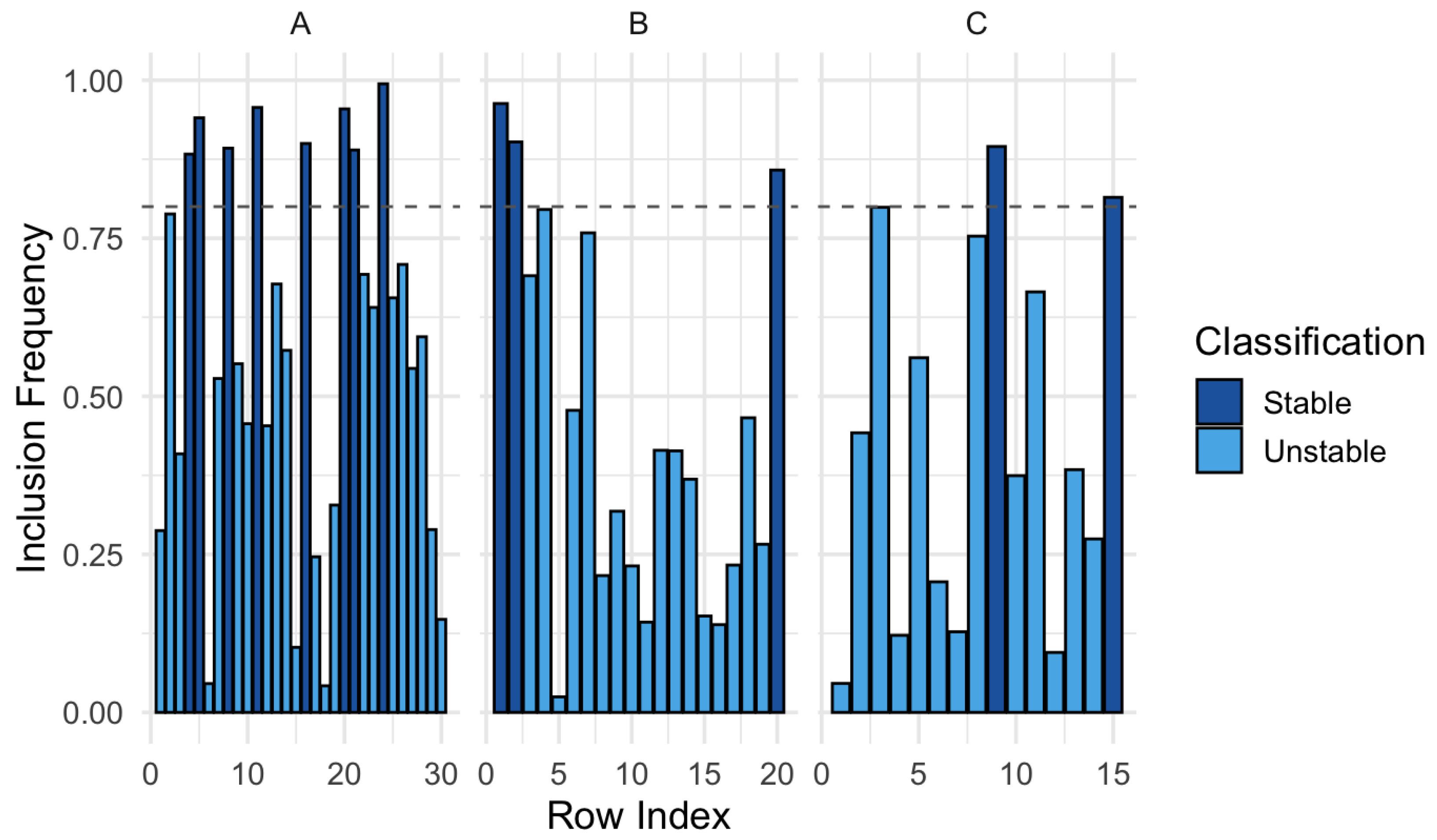
Each bar in Figure 7 represents the inclusion frequency of a tensor row in the penalized support across bootstrap replicates. The figure allows for an immediate visualization of structural consistency by mode: mode concentrates a larger number of stable inclusions, in contrast to modes and , which exhibit greater dispersion. This pattern reinforces the value of the SSI as a post-penalization metric that filters reliable support, particularly useful in contexts with high collinearity or risk of overfitting.
In addition to the absolute value of the SSI, it is useful to express this result in relative terms with respect to the total number of rows available per mode. The proportion of stable support is defined as:
This metric allows for the comparison of the relative density of stability across modes, even when they differ in dimensionality. In the observed results, mode reaches a stability proportion of 45%, while modes and C remain below 30%, reinforcing the notion of greater structural robustness in the first mode.
This normalized form of the SSI has been suggested as a standardized interpretation mechanism in Stability Selection (Meinshausen & Bühlmann, 2010) and has been applied in subsequent work on reproducible selection in high-dimensional settings (Shah & Samworth, 2013).
2.6. Standard Deviation of Support Size
In addition to evaluating which elements are selected recurrently, it is crucial to analyze the stability in the number of elements selected. In penalized models such as LASSO or Elastic Net, it is common for the size of the support to vary across replicates, especially under conditions of collinearity or weak signal-to-noise ratio (Zou and Hastie, 2005; Meinshausen and Bühlmann, 2010).
To capture this variability, the standard deviation of the support size across the bootstrap replicates is computed as:
where
Here, represents the cardinality of the support obtained in replicate bbb, while is its average value. This metric summarizes the model’s quantitative fluctuation, even if the selected elements are partially consistent. A high value of indicates that the model changes size unstably, which compromises its structural reproducibility. In contrast, a value close to zero suggests consistent parsimony, a desirable property in high-dimensional settings.
The importance of this metric has been recognized in studies on structural regularization (Shah and Samworth, 2013) and post-penalization validation (Bach, 2008), where variability in size is seen as a sign of sensitivity.
Figure 8 presents the distribution of the penalized support size obtained in each bootstrap replicate, distinguishing the three tensor modes. It can be observed that mode not only has a larger average support size, but also shows lower dispersion, which reinforces its structural stability. In contrast, modes and show greater variability in the selected cardinality, which may be due to collinearity, weaker latent signal, or sensitivity to the regularization parameter.
Figure 7.
Boxplot of Support Size by Mode (Cardinality Variability).
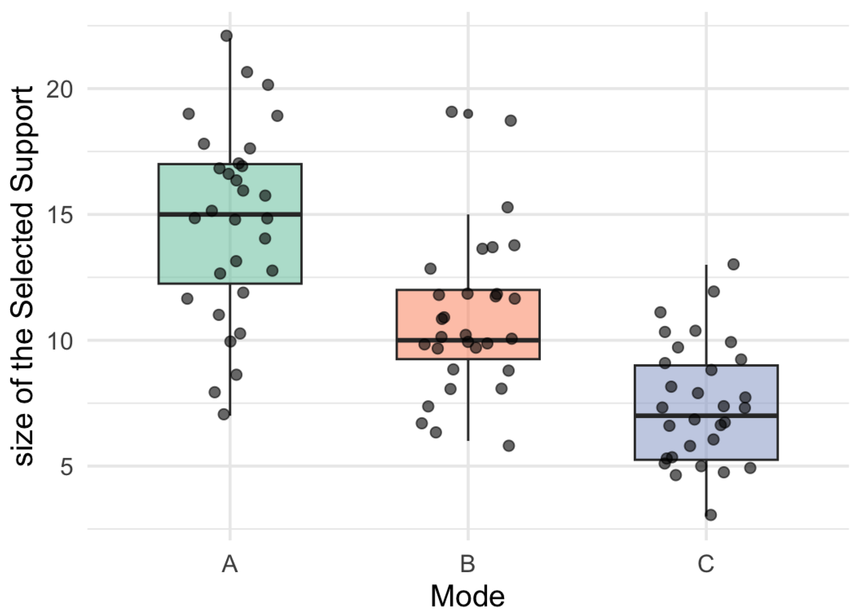
This metric provides a complementary view to inclusion frequencies and the SSI, allowing us to analyze not only which rows are selected but how many are consistently selected. The standard deviation of cardinality thus becomes an essential criterion for evaluating the stability of the penalized model in multiway contexts (Bach, 2008; Shah and Samworth, 2013).
The metrics developed in this section — inclusion frequency, Jaccard index, stable selection index (SSI), standard deviation of support size, and proportion of stable support — allow for a comprehensive characterization of the structural behavior of the CenetTucker model (González-García, 2019) fitted with Elastic Net penalization throughout the resampling process. Unlike approaches focused solely on minimizing reconstruction error, these metrics evaluate key structural properties such as support consistency, stability under perturbations, and multiway robustness in high-dimensional contexts.
Support consistency, stability under perturbations, and multiway robustness in high-dimensional contexts.
This framework is inspired by previous developments such as Stability Selection (Meinshausen and Bühlmann, 2010), Bolasso (Bach, 2008), and their recent extensions in the field of structured penalization (Shah and Samworth, 2013), adapting these principles to the tensor setting through a specific resampling protocol on the observational mode. Each metric offers a complementary perspective: from pointwise inclusion to global dispersion, including binary filters such as the SSI, which have proven useful in improving interpretability in complex penalized models (Bühlmann and van de Geer, 2011).
This set of evaluative tools constitutes the empirical foundation upon which the performance of the CenetTucker model will be analyzed in a simulated environment in the following section. This application will clearly illustrate how the quantified stability properties manifest and will provide concrete evidence on the value of the proposed approach.
The complete protocol has been implemented in the GSparseBoot package, publicly available on GitHub (see Appenix 1), which ensures reproducibility and facilitates its application in real-world contexts.
3. Application to Simulated Data
In order to illustrate the structural behavior of the CenetTucker model and evaluate the impact of bootstrap on its stability, a controlled simulation has been designed based on tensor data with known latent structure. This application has a didactic purpose: to intuitively and reproducibly demonstrate how the developed metrics allow for diagnosing instability and quantifying reliable support in a high-dimensional setting.
A three-dimensional tensor χ was generated, where corresponds to the number of observations (mode-1), to the variables (mode-2), and to the experimental conditions (mode-3). The internal structure of the tensor was simulated using a Tucker model with reduced rank (, with a core tensor generated with independent entries drawn from a standard normal distribution.
The loading matrices were randomly generated with Gaussian entries , and subjected to row-wise masking to induce controlled sparsity. This construction makes it possible to know in advance the location of relevant rows, which is essential for evaluating the model’s behavior.
The simulated tensor is obtained as:
where represents an additive noise tensor with independent Gaussian entries and is set as the level of unstructured variability.
Based on this simulated design, the CenetTucker model was fitted without applying bootstrap, to observe its structural stability under identical input conditions but with slight random variations. The results obtained allow for an empirical evaluation of the model’s sensitivity and serve as a baseline to contrast the stabilizing effect of resampling.
3.1. Empirical Evaluation of CenetTucker Instability
To assess the structural stability of CenetTucker in the absence of resampling mechanisms, independent runs were performed on the same simulated tensor. Each run kept the penalization hyperparameters and constant, varying only the random seed and introducing slight perturbations in the noise component, in order to simulate realistic conditions of minimal sample variability.
After each fit, the penalized support sets were extracted—that is, the active rows with at least one non-zero coefficient—from the loading matrices . Table 2 presents a statistical summary of the support cardinalities obtained:
This variability is clearly visualized in Figure 9 through a boxplot by mode:
Figure 8.
Boxplot of Cardinality by Mode.
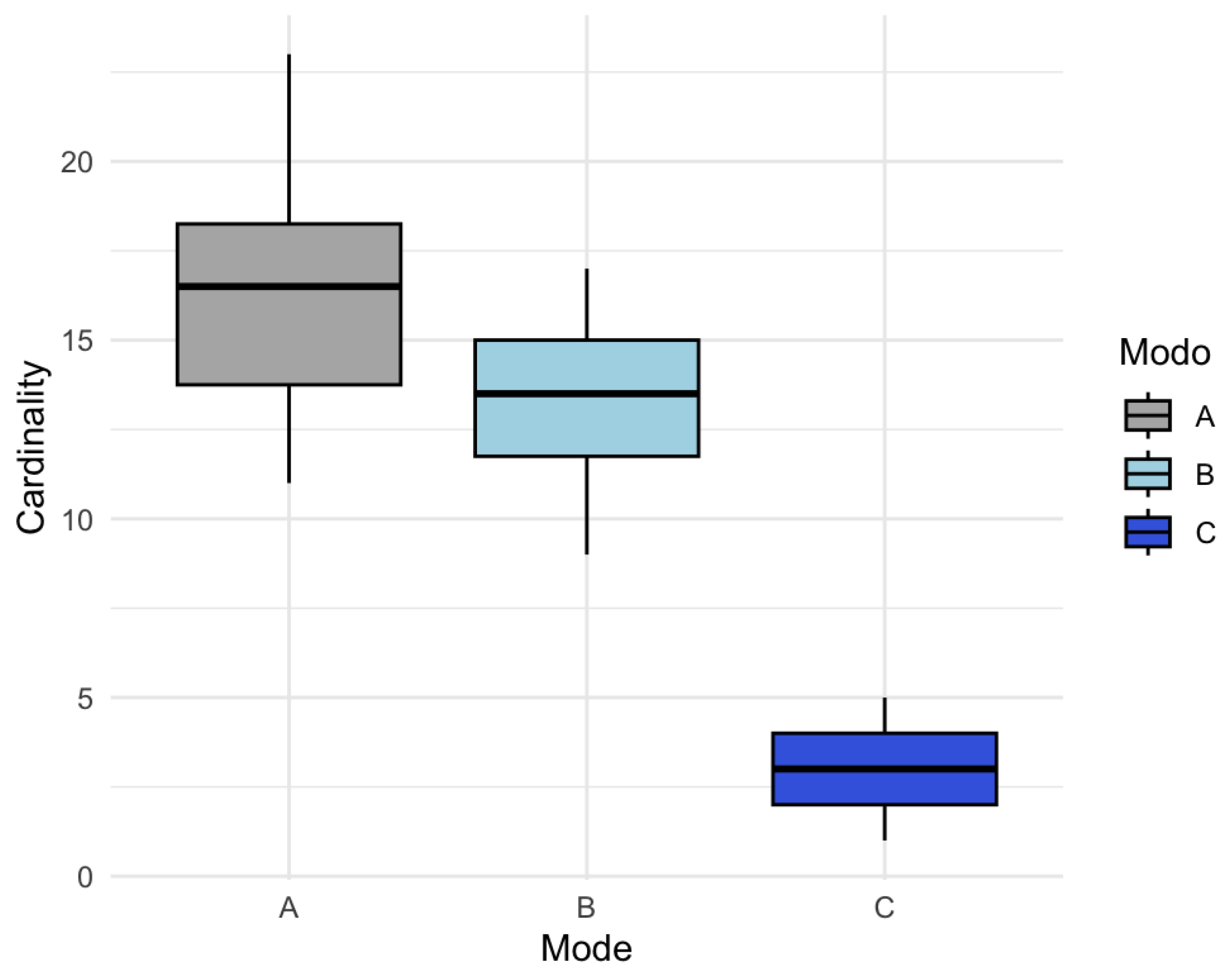
In the boxplot (Figure 9), mode shows the largest average support size, but also substantial dispersion (a range of 12 units), reflecting sensitivity to random perturbations. Mode , although with a lower mean, displays similar variability. In mode , despite its low cardinality, a proportionally important dispersion persists. These patterns suggest that the selected structure is unstable and dependent on uncontrolled factors.
Additionally, the Jaccard index was calculated between all possible pairs of runs for each mode in order to quantify the structural overlap between the selected support sets. Figure 10 shows the distribution of these indices for mode :
The results indicate that most Jaccard values are concentrated below 0.3, with an average of approximately 0.25. This implies that, on average, fewer than 30% of the rows selected as relevant overlap between different runs of the model, revealing a pronounced structural instability. This behavior confirms findings reported in the literature on penalized models without structural validation (Meinshausen and Bühlmann, 2010; Shah and Samworth, 2013; Yu et al., 2019).
This set of results demonstrates that even under controlled simulation conditions, the CenetTucker model—when fitted directly without structural validation mechanisms—exhibits marked instability in sparse support selection. The observed sensitivity to minor perturbations or random variations in noise compromises both the statistical reproducibility and the structural interpretability of the latent factors.
In response to this limitation, the following section proposes a bootstrap protocol specifically adapted to CenetTucker, designed to assess and improve its stability. This approach will allow for empirical quantification of the selection frequency of each row, identification of structural consistency patterns, and definition of robust stability metrics that distinguish reliable support from noise introduced by penalization or resampling.
3.2. Application of Bootstrap to CenetTucker
In order to evaluate the impact of bootstrap on the structural stability of the CenetTucker model, the previously designed resampling protocol was applied, focused on mode-1 (observations), while keeping the latent structure and penalization hyperparameters constant.
A total of bootstrap replicates were generated from the simulated tensor. In each replicate , the CenetTucker model was fitted using the same values of y defined in the previous section, without recalibrating the hyperparameters for each replicate. The goal of this configuration is to determine whether resampling alone—while preserving the penalization—can induce improvements in structural stability.
For each replicate, the sparse supports from the loading matrices , , were extracted. From these sets, the following metrics were calculated: inclusion frequency of each row, Jaccard index between all pairs , stable selection index (SSI) for each mode, proportion of stable support by mode, and standard deviation of the cardinalities for each mode.
The results were directly compared to the previous phase (without bootstrap), using the standard deviation of support sizes and the average Jaccard index as reference metrics. In particular:
The table provides a quantitative summary of the impact of bootstrap on the stability of the CenetTucker model. The metrics compared are grouped into three key dimensions: support variability, structural consistency, and systematic selection stability.
- A.
- Variability in Support Size (Standard Deviation by Mode):
The standard deviation of the sparse support cardinality decreases substantially when bootstrap is applied. In mode , it is reduced from 3.50 to 1.82; in mode , it decreases from 3.33 to 2.01; and in mode , it drops from 1.42 to 0.89. This reduction indicates that bootstrap acts as a stabilizing mechanism by generating more homogeneous selections across replicates.
This reduction indicates that bootstrap acts as a stabilizer by generating more homogeneous selections across replicates.
As shown in Figure 11, the dispersion in the number of rows selected per replicate decreased considerably after applying bootstrap. This reduction is especially notable in modes and , where the boxplot boxes are more compact and centered. This indicates greater structural homogeneity in the solutions obtained.
- B.
- Structural agreement across runs (Average Jaccard Index):
The average Jaccard index improves significantly across all three modes. In mode , it increases from 0.209 to 0.412 (an increase of nearly 100%); in mode , it rises from 0.265 to 0.398; and in mode , it goes from 0.222 to 0.379.
These increases reflect a higher level of agreement between the obtained support sets, supporting improved structural reproducibility of the penalized model.
Figure 12 shows the distribution of the Jaccard index across pairs of bootstrap replicates. In contrast to the non-bootstrap scenario, the values shift to the right, reaching an average of 0.41 in mode . This increase quantifies the improvement in structural reproducibility induced by resampling.
- C.
- Systematic stability (SSI and stable proportion): Before applying bootstrap, CenetTucker does not identify any row as consistently selected (SSI = 0 in all modes). After bootstrap: in mode , 28 stable rows are identified, representing 56% of the total; in mode , 11 stable rows are identified (37%); and in mode , 3 stable rows are selected (30%).
This evidence suggests that the bootstrap protocol not only reduces variability, but also filters a reliable subset of the support, empirically distinguishing between structural signal and noise.
Before applying bootstrap, the model did not identify any row as consistently selected. In contrast, after its application, the SSI reveals substantial improvements, visualized in Figure 13, where the green bars indicate rows selected with high frequency. A more stable and differentiated selection pattern between signal and noise is observed.
Complementarily, Figure 14 shows the proportion of stable support by mode. Mode A shows a proportion of 56%, followed by mode B (37%) and mode C (30%). These figures support that the bootstrap protocol not only reduces variability but also filters a reliable subset of the support, enhancing the interpretative robustness of the CenetTucker model.
4. Discussion
The results presented in this study expand and critically consolidate the methodological framework proposed by González-García (2019), who introduced the CenetTucker model as a sparse extension of classical Tucker, applying Elastic Net penalization to the loading matrices. While this formulation represented a step forward in incorporating structured sparsity in multiway contexts, its limitations in terms of stability had not been systematically quantified. This work provides strong empirical evidence that CenetTucker, in its original form, is prone to producing structurally unstable solutions, highly sensitive to random perturbations or algorithm initialization.
This finding aligns with that reported by Meinshausen and Bühlmann (2010), who showed that in penalized models, small sample variations can significantly alter the selected support sets, undermining reproducibility. Yu et al. (2019) also warned about the fragility of sparse models when fitted without structural validation—an issue extended here for the first time to the tensor framework.
In response, the implementation of a bootstrap protocol adapted to CenetTucker constitutes a methodological innovation that, much like the Stability Selection method proposed by Shah and Samworth (2013), introduces an additional layer of robustness without modifying the model’s structure. In our case, resampling over mode-1 combined with the computation of metrics such as inclusion frequency, Jaccard index, and SSI has been shown to improve the model’s structural stability across at least three key dimensions: reduction of variability, increase in support overlap across replicates, and emergence of reliable support subsets.
This result not only reinforces Bach’s (2008) proposition regarding the usefulness of bootstrap in sparse models but also shows that its extension to the tensor domain is viable, useful, and measurable. Unlike solutions obtained directly through penalization—which exhibit high dispersion and low reproducibility—the proposed bootstrap protocol acts as an empirical filter that identifies persistent structural patterns, significantly enhancing the interpretability of the selected factors.
From a practical standpoint, this approach is particularly valuable in fields where reproducibility is critical, such as computational biology, transcriptome analysis, or neuroimaging, where data exhibit multiway structure and errors in variable selection may have substantial implications.
However, this study has focused exclusively on classic bootstrap applied to the observational mode. Several relevant lines remain open for future research: the incorporation of residual and Bayesian bootstrap in tensor settings (as already partially explored in linear regression), evaluation of the protocol’s sensitivity to different noise levels, and integration with adaptive hyperparameter selection strategies.
Studies Limitations
Despite the favorable results obtained, it is important to acknowledge certain limitations of the proposed approach:
- Dependence on the type of resampling: The developed protocol is based on classical bootstrap over the observational mode. While this preserves the tensor’s multiway structure, it does not consider residual or parametric resampling, which could capture different sources of variability. Exploring these alternatives remains a direction for future development.
- Non-recalibrated hyperparameters per replicate: In this version, the penalization hyperparameters are fixed across all bootstrap replicates. While this isolates the effect of resampling, the lack of recalibration may limit the support’s fine-tuning in more complex or heterogeneous contexts. An extension with replicate-specific adaptive selection could further enhance robustness.
- Evaluation on simulated data: Although the simulated setting allows full control over the latent structure and facilitates quantitative validation, no direct application to real data was included. This temporarily limits the generalizability of the findings, although the protocol is designed for empirical implementation.
- Computational scalability: The current implementation of the GSparseBoot package in R is efficient for tensors of moderate size, but execution on large datasets or with a high number of replicates may require parallelization or further optimization, especially in memory-constrained environments.
- Lack of benchmarking against other stabilization methods: Although the article focuses on the bootstrap versus non-bootstrap contrast, results were not compared with alternative stable selection methods such as Stability Selection (Meinshausen and Bühlmann, 2010) or Bayesian approaches, which may be addressed in future work.
5. Conclusions
This article presents a rigorous methodological proposal to address one of the main challenges in penalized tensor models: the structural instability of sparse support. Through a bootstrap protocol adapted to the CenetTucker model, it was possible to quantify, reduce, and reinterpret the variability associated with the loading matrices obtained in high-dimensional contexts.
The main findings can be summarized as follows:
- The CenetTucker model, in its original formulation, is prone to generating unstable solutions, even under small sample perturbations. This instability affects result reproducibility and complicates the interpretation of factor loadings, compromising the model’s utility in real-world applications.
- Applying bootstrap over the observational mode enables empirical stabilization of the penalized support without recalibrating hyperparameters, distinguishing persistent signal from random noise. The proposed metrics—inclusion frequency, Jaccard index, stable selection index (SSI), and stable proportion—provide a rigorous framework for assessing this stability.
- It was empirically shown that the bootstrap protocol reduces support variability (by up to 50%), doubles the overlap between replicates (average Jaccard index), and yields robust support subsets with more than 50% of rows classified as stable in the most consistent mode.
- As a computational contribution, this work introduces the GSparseBoot library, developed in R and available on GitHub, which implements the complete protocol for resampling, penalized fitting, support extraction, and stability metric calculation. This tool facilitates reproducibility, transparency, and the extension of the proposed approach, serving as a starting point for new applications and developments in real-world settings (see Appendix A).
- Overall, these results provide a concrete, reproducible, and extensible solution to the problem of instability in sparse multiway models, contributing to both methodological development and practical implementation.
Appendix A
Due to the lack of an existing solution that combines Elastic Net penalization, tensor structures, bootstrap resampling, and stability evaluation, this research proposes the development of the GSparseBoot package.
GSparseBoot not only automates the entire penalized modeling process for tensor data, but also integrates stability validation modules that, until now, were not available in any single package. Its modular architecture allows for extension to new penalization methods, selection criteria, or resampling schemes, making it an open tool for research in applied computational statistics.
This library, implemented in R, automates the complete analysis pipeline for sparse models with bootstrap-based stabilization and includes:

Table A1.
GsparseBoot Structure.
| ⊢ simulate_tensor.R # Simulates sparse tensors with noise |
| ⊢ elastic_net_tensor.R # Fits Elastic Net on matricized tensor |
| ⊢ bootstrap_tensor.R # Executes bootstrap (classic, residual, parametric) |
| ⊢ stability_metrics.R # Calculates frequency, Jaccard, variability, stability index |
| ⊢ print/summary/plot # S3 methods for visualization |
| ⊢ vignettes/ # Use case examples with simulated and real data |
| ⊢ tests/ # Automated tests using testthat |
| ⌞ pkgdown/ # n of the package |
Each function is documented using roxygen2 and includes reproducible examples. Output from each module is structured as S3 class objects (“GSparseModel” or “GSparseBootstrap”), allowing for straightforward extensibility and validation.
GSparseBoot Componente
simulate_tensor()
Generates a three-dimensional tensor with Tucker structure, adds controlled noise, and applies a sparsity mask.
elastic_net_tensor()
Unfolds the tensor along mode-n, standardizes the data, and fits Elastic Net using glmnet. Selects via Cross-validation, AIC, BIC, or eBIC. Returns coefficients, support, and penalized tensor reconstruction.
bootstrap_tensor()
Performs resamples of the specified type (classic, residual, parametric). Applies elastic_net_tensor() to each replicate and aggregates the selected supports.
stability_metrics()
Calculates inclusion frequency, Jaccard index, support variability, and the stable selection index.
Table A2.
Summary of the Structural Tree with GSparseBoot Module Paths.
| Función | Propósito | Entrada Principal | Salida principal |
|---|---|---|---|
| simulate_tensor() | Simulate sparse tensor with noise and controlled rank | dims, noise, sparsity | |
| elastic_net_tensor() | Fit Elastic Net penalization on matricized modes | coefficients and reconstruction | |
| bootstrap_tensor() | Generate B resamples and apply per-replicate fitting | tensor, B, bootstrap.type | list of supports |
| stability_metrics() | Compute stability metrics | list of supports | matriz de métricas (freq, SSI) |
Legend: Simulation: Generation of synthetic data with known structure. Penalization: Elastic Net fitting and selection of λ. Bootstrap: Resampling and reevaluation of support. Stability: Computation of comparative stability metrics.
Figure 14.
GsparseBoot Structure as Package.
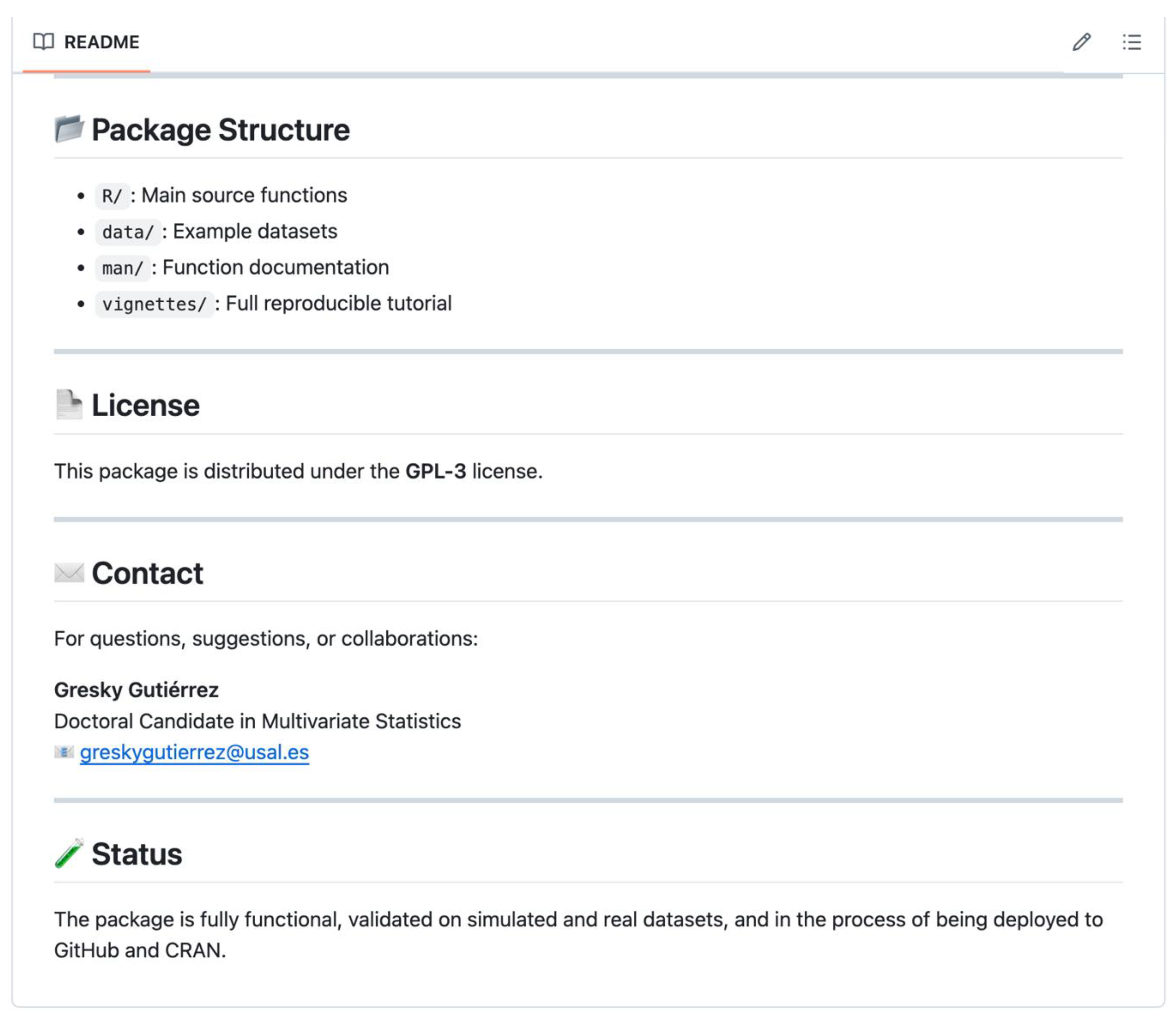
Figure 15.
GsparseBoot en HitHub.
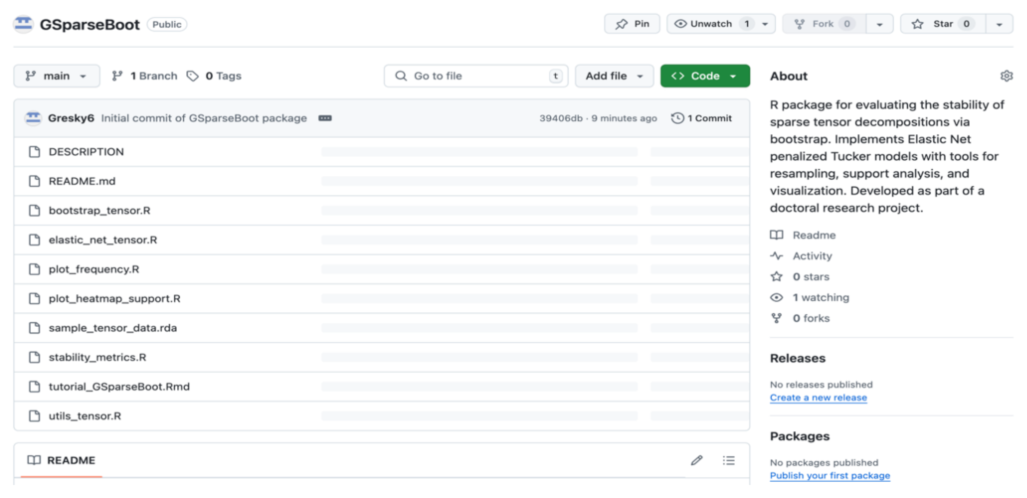
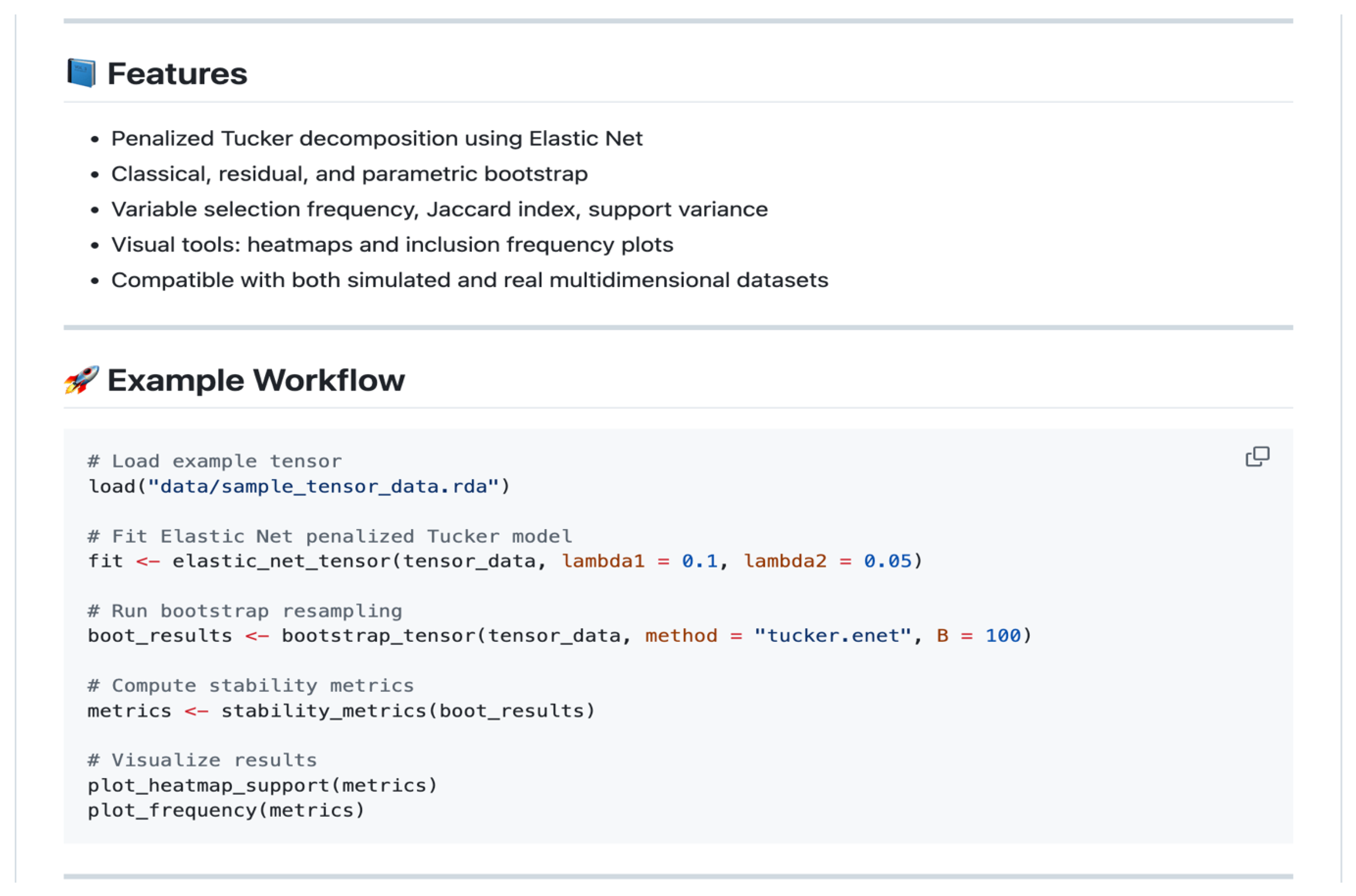
Figure 16.
GSparseBoot Features and workflow example.
References
- Bach, F. (2008). Bolasso: Model consistent Lasso estimation through the bootstrap. Proceedings of the 25th International Conference on Machine Learning, 33–40. [CrossRef]
- Bühlmann, P., & Van De Geer, S. (2011). Statistics for high-dimensional data: Methods, theory and applications. Springer. [CrossRef]
- Efron, B. (1979). Bootstrap methods: Another look at the jackknife. The Annals of Statistics, 7(1), 1–26. [CrossRef]
- González-García, L. (2019). Regularización en modelos tensoriales: Una aproximación mediante penalización tipo Elastic Net [Doctoral dissertation, Universidad de Salamanca].
- Hastie, T., Tibshirani, R., & Friedman, J. (2009). The elements of statistical learning: Data mining, inference, and prediction (2nd ed.). Springer. [CrossRef]
- Kolda, T. G., & Bader, B. W. (2009). Tensor decompositions and applications. SIAM Review, 51(3), 455–500. [CrossRef]
- Meinshausen, N., & Bühlmann, P. (2010). Stability selection. Journal of the Royal Statistical Society: Series B (Statistical Methodology), 72(4), 417–473. [CrossRef]
- Shah, R. D., & Samworth, R. J. (2013). Variable selection with error control: Another look at Stability Selection. Journal of the Royal Statistical Society: Series B (Statistical Methodology), 75(1), 55–80. [CrossRef]
- Tibshirani, R. (1996). Regression shrinkage and selection via the lasso. Journal of the Royal Statistical Society: Series B (Methodological), 58(1), 267–288. [CrossRef]
- Yu, B., Wang, Y., Samworth, R., & Hastie, T. (2019). Stability in feature selection. Annals of Statistics, 47(3), 1739–1762. [CrossRef]
- Zou, H., & Hastie, T. (2005). Regularization and variable selection via the elastic net. Journal of the Royal Statistical Society: Series B (Statistical Methodology), 67(2), 301–320. [CrossRef]
- Zhou, H., Li, L., & Zhu, H. (2013). Tensor regression with applications in neuroimaging data analysis. Journal of the American Statistical Association, 108(502), 540–552. [CrossRef]
Figure 1.
Tucker Decomposition (adapted from Tucker, 1966).
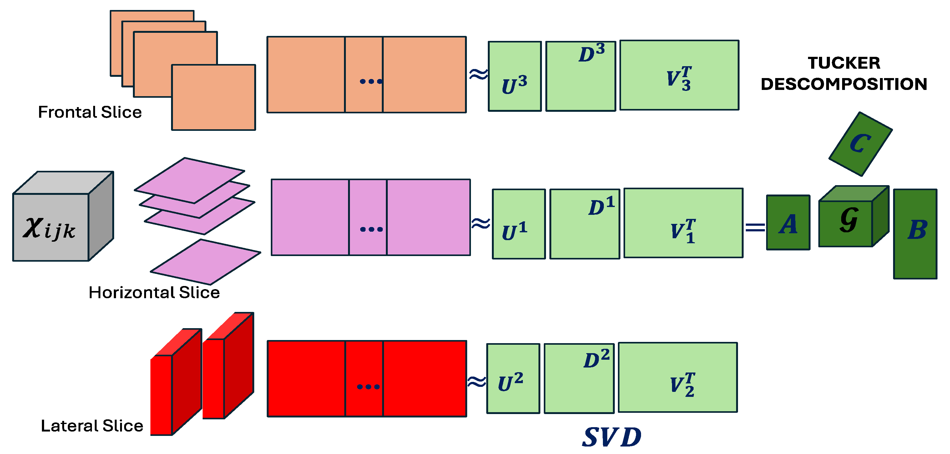
Figure 2.
CenetTucker representation (adapted from González-García, 2019).
Figure 3.
Comparative visualization between Tucker and CenetTucker (produced by the authors).
Figure 5.
Representation of Inclusion Frequency.

Figure 6.
Jaccard Index Matrix Across B Bootstrap Replicates.
Figure 9.
Distribution of the Jaccard Index Across Runs (Mode A).
Figure 10.
Dispersion of Support Cardinality by Mode (with Bootstrap).
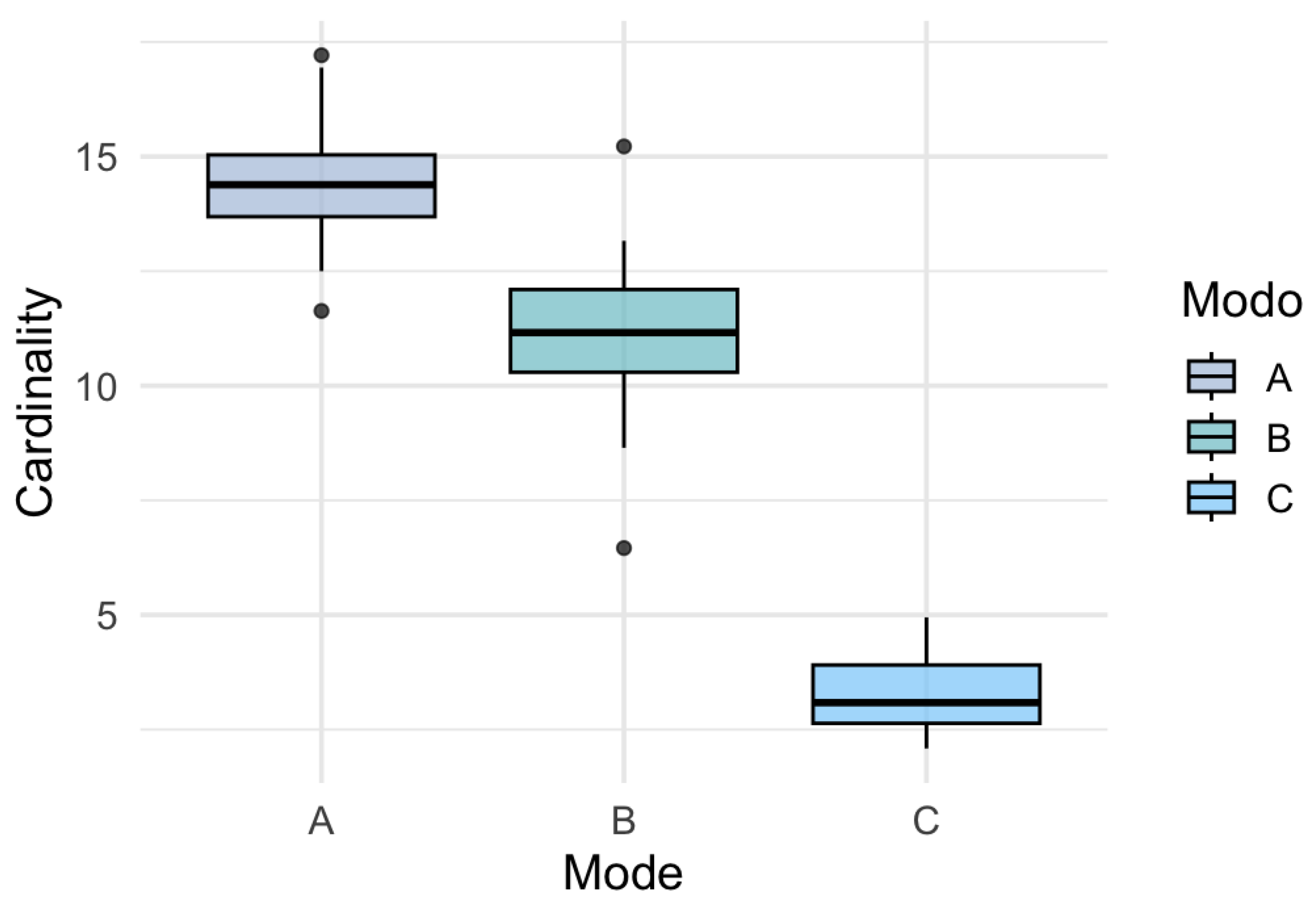
Figure 11.
Distribution of the Jaccard Index Across Bootstrap Replicates.
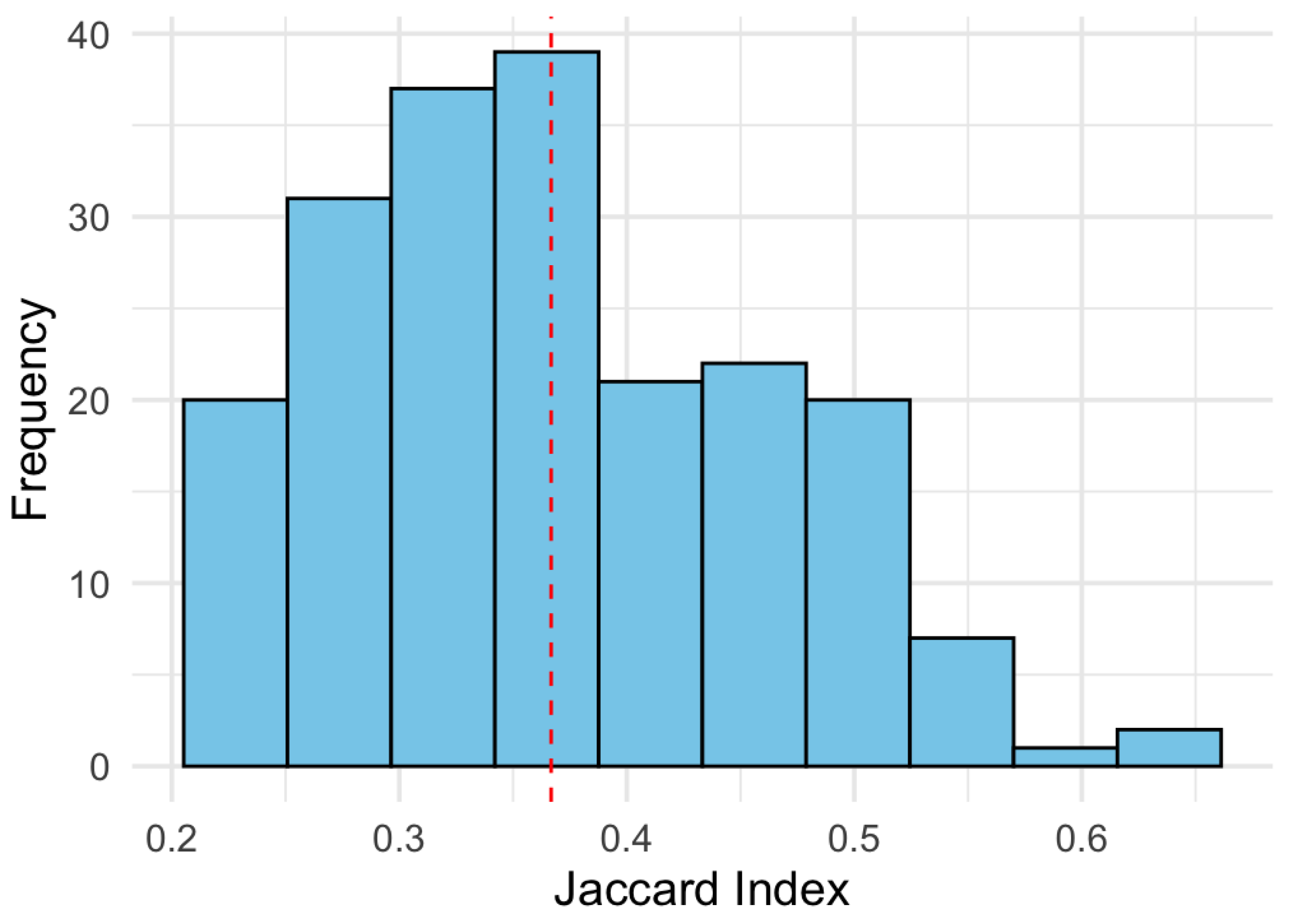
Figure 12.
Stable Selection Index.
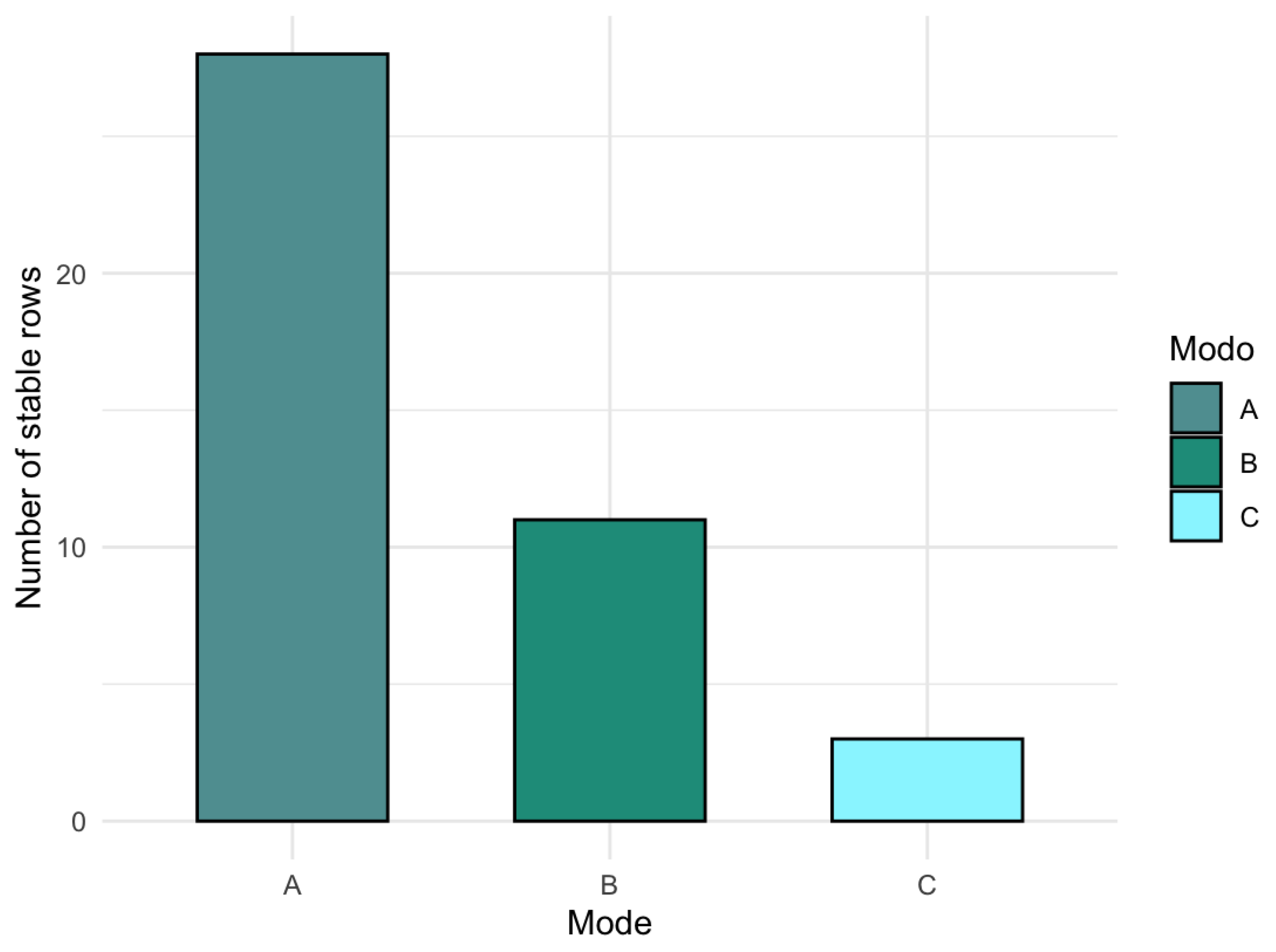
Figure 13.
Proportion of Stable Support by Mode.
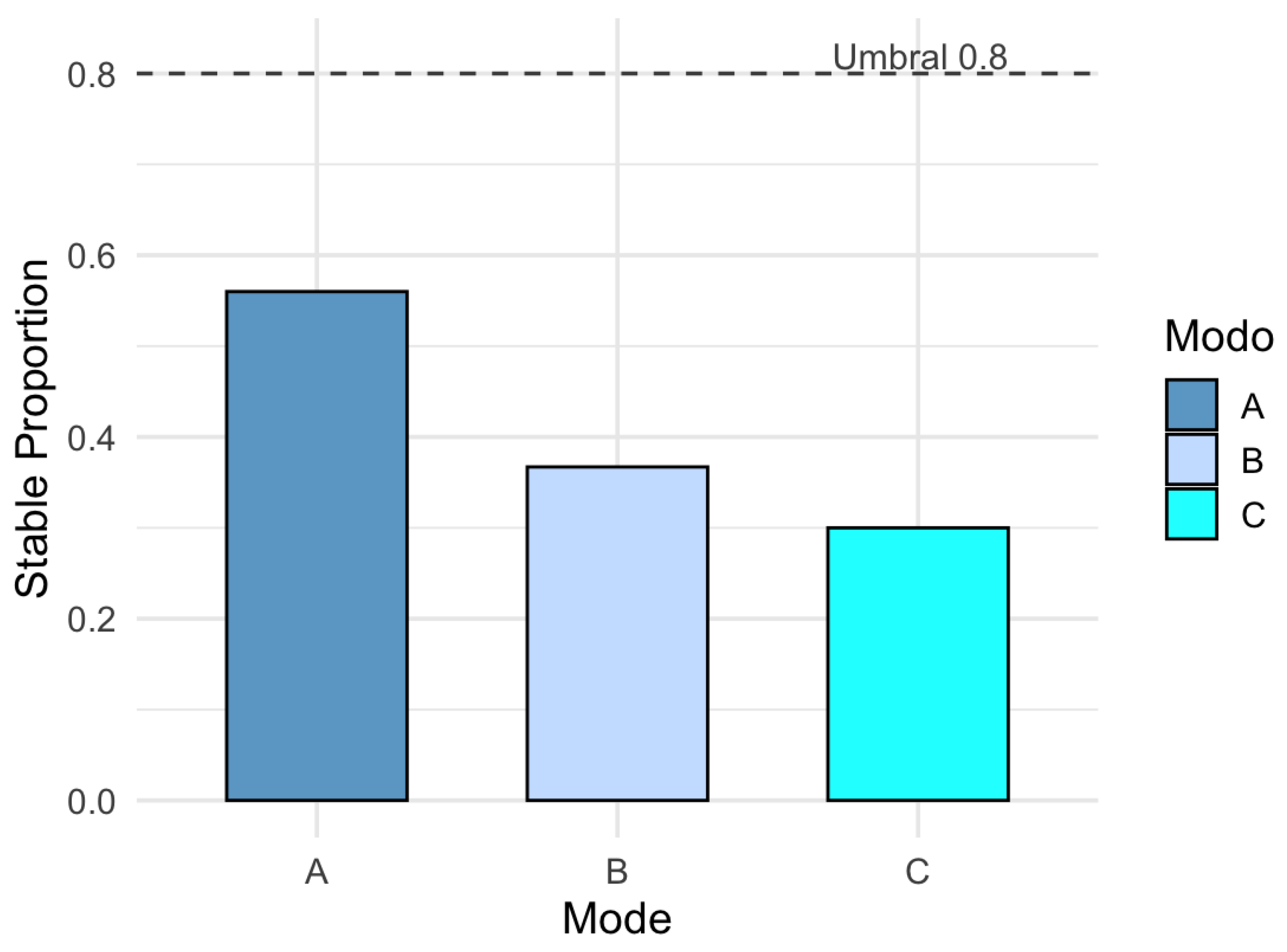
Table 1.
Classical Bootstrap Algorithm.
| Algorithm: Non-Parametric Bootstrap |
| Input: Sample , number of replications B, statistic of interest |
| Salida: Empirical distribution of , bias estimates, standard error, and confidence intervals. |
| 1. to B, do: Generate Bootstrap samples by sampling with replacement from the original data of size n. Compute the Bootstrap statistic: From the set an empirical distribution is obtained for inference, bias evaluation, standard error, confidence interval estimation, or—as in this study—stability analysis. End of loop |
| Compute the Bootstrap mean: Compute the standard error: Estimate the percentile confidence interval: |
Table 2.
Statistical summary of support cardinality in 20 runs of the CenetTucker model.
| Mode | Mean | Minimum | Maxumim | Standard devition |
|---|---|---|---|---|
| A | 16.05 | 11 | 23 | 3.50 |
| B | 11.95 | 7 | 17 | 3.33 |
| C | 3.15 | 1 | 5 | 1.42 |
Table 3.
Resultados comparativos de estabilidad.
| Metric | Without Bootstrap (Average) | With Bootstrap (Average) |
|---|---|---|
| Standard Deviation (A) | 3.500 | 1.820 |
| Standard Deviation (B) | 3.330 | 2.010 |
| Standard Deviation (C) | 1.420 | 0.890 |
| Average Jaccard (A) | 0.209 | 0.412 |
| Average Jaccard (B) | 0.265 | 0.398 |
| Average Jaccard (C) | 0.222 | 0.379 |
| SSI (A) | 0 | 28 |
| SSI (B) | 0 | 11 |
| SSI (C) | 0 | 3 |
| Stable Proportion (A) | 0.000 | 0.560 |
| Stable Proportion (b) | 0.000 | 0.367 |
| Stable Proportion (C) | 0.000 | 0.300 |
Disclaimer/Publisher’s Note: The statements, opinions and data contained in all publications are solely those of the individual author(s) and contributor(s) and not of MDPI and/or the editor(s). MDPI and/or the editor(s) disclaim responsibility for any injury to people or property resulting from any ideas, methods, instructions or products referred to in the content. |
© 2025 by the authors. Licensee MDPI, Basel, Switzerland. This article is an open access article distributed under the terms and conditions of the Creative Commons Attribution (CC BY) license (http://creativecommons.org/licenses/by/4.0/).
Copyright: This open access article is published under a Creative Commons CC BY 4.0 license, which permit the free download, distribution, and reuse, provided that the author and preprint are cited in any reuse.


