Submitted:
29 May 2025
Posted:
30 May 2025
You are already at the latest version
Abstract
An expanded Pacific Earthquake Engineering Research (PEER) Center Next Generation Attenuation Phase 2 (NGA-West2) ground motion database compiled from shallow crustal earthquakes in active crustal regions (ACR) is used to develop closed form GS24b backbone ground motion model (GMM) for the “average” RotD50 horizontal components of peak ground acceleration (PGA), peak ground velocity (PGV) and 5% damped elastic pseudo-absolute response spectral accelerations (SA). GS24b model is applicable to earthquakes with moment magnitudes 4.0 ≤ M ≤ 8.5, at rupture distances of 0 ≤ Rrup ≤ 400 km, with time-averaged S-wave velocity in the upper 30 m of the profile 150 ≤ VS30 ≤1500 m/s, and for periods 0.01 ≤ T ≤10 s. The new backbone model includes VS30 site correction developed based on multiple representative S-wave velocity profiles. For crustal waves attenuation we are using apparent anelastic attenuation of SA -- QSA (f, M). In contrast to the GK17 the GS24b backbone is a generic ACR model designed specifically to be adjusted to any ACRs. The GS24bc is an example of a partially non-ergodic model created by adjusting the backbone GS24b model for magnitude M, S-wave velocity VS30 and fault rupture distance Rrup residuals.
Keywords:
Closed form backbone ground motion model
; active crustal region
; NGA-West2
; Turkey 2023 earthquakes
1. Introduction
Ground motion models (GMMs) also called ground motion prediction equations (GMPEs), or originally attenuation relations, use datasets of recorded ground motion parameters at multiple seismic stations during different earthquakes and in various seismic source regions in a similar tectonic environment to generate equations. These equations are later used to estimate site-specific ground motions that may shake a site if an earthquake of a certain magnitude occurs at a nearby location. These models describe the distribution of ground motion in terms of a median and a logarithmic standard deviation and are crucial in assessing seismic hazard, thereby providing estimates of the loading that a structure may undergo during a future earthquake.
Typically, Ground Motion Models are developed using an empirical regression of observed amplitudes against an available set of predictor variables. Joyner and Boore [1,2] proposed performing analyses of data using the two-stage regression based on the algorithm [3,4] for applying the random effects model to regression analyses. Abrahamson and Youngs [5] presented an alternative mixed-effects algorithm that is more stable according to the authors although computationally less efficient. In these approaches, coefficients were obtained separately for each period resulting in response spectra that demonstrates jaggedness and consequently requiring smoothing (e.g., [6,7,8,9]).
In contrast to the above-described traditional approaches, we are using the non-traditional approach first introduced by Graizer and Kalkan [10,11,12] and later expanded in [13,14]. In this method at the first stage the closed form expression of the two functions (peak ground acceleration and spectral shape ) composition is developed separately for the active crustal and stable continental regions (ACR and SCR) approximating ground motion attenuation. This type of modeling was originally based on the expanded NGA-West1 dataset and is developed using the Nelder-Mead method of nonlinear minimization [15]. However, this closed form approximation is not flexible enough to describe all variations of response spectral attenuation and to produce lower standard error. This is why we incorporated the second stage when previously developed closed form generic model is adjusted based on residuals for each period.
In [16] the new set of strong motion data from the two strongest 2023 earthquakes in Turkey were used to test the ergodic GK17 GMM [14]. The GK17 model developed using the NGA-West2 database [17] for the active crustal regions was applied to the dataset of recordings from the two moment magnitude 7.8 and 7.5 earthquakes in Turkey [18,19]. The GK17 model demonstrates acceptable performance while mostly underpredicting spectral accelerations at near fault up to ~100 km and far-field more than ~400 km rupture distances for short periods s. In [16] GK17 model was modified by applying additional distance and residuals corrections creating an updated GK model tuned for Turkey and called the GK_T model. Turkey specific GK_T partially non-ergodic model shows better agreement with recorded data than the ergodic GK17 model, especially at short periods and most importantly short rupture distances.
We recently developed two new GMMs [20]:
- The global backbone GS24b model that uses the closed form approximation of the spectral acceleration as a multiplication of the and spectral shape (normalized spectral acceleration spectrum) functions. This model can be later used for adjusting to the specific ACR region (e.g., Southern and Northern California) creating partially non-ergodic models.
- The ergodic GS24 model representing the backbone GS24b GMM adjusted for the depth to the shear-wave velocity horizon of 2.5 km/s (), style of faulting () and also for the moment magnitude , time-averaged shear-wave velocity in the upper 30 meters and closest distance to the fault rupture residuals.
In this paper we are presenting the backbone model GS24b and the GS24bc model created by adjusting backbone model for residuals. We also tested previously developed GK17 GMM [14] against the NGA-West2 dataset expanded with recordings from the three 2023 strong Turkish earthquakes.
2. Datasets
The new GS24b model is based on Pacific Earthquake Engineering Research (PEER) Center Next Generation Attenuation Phase 2 (NGA-West2) data expanded with recordings from the three 2023 Turkish earthquakes with moment magnitudes of 6.3, 7.5 and 7.8 [18,19] ground motion database compiled from shallow crustal earthquakes in active crustal regions to develop a GMM for the “average” RotD50 (50th percentile or median response [21] horizontal components of peak ground acceleration (), peak ground velocity () and 5% damped elastic pseudo-absolute acceleration response spectral ordinates () at 21 oscillator periods (T) ranging from 0.01 to 10 sec [17]. The specific spectral periods are 0.01, 0.02, 0.03, 0.05, 0.075, 0.1, 0.15, 0.2, 0.25, 0.3, 0.4, 0.5, 0.75, 1, 1.5, 2, 3, 4, 5, 7.5 and 10 sec. This set of periods is considered to be representative in current US engineering practice. The number of predictors used in the current model is limited to a few measurable parameters: moment magnitude (), closest distance to the fault rupture plane ( time-averaged shear-wave velocity in the upper 30 m of the geological profile (), and apparent (intrinsic and scattering) attenuation factor ) of 5% damped spectral acceleration.
The currently used dataset consists of the original subset of the NGA-West2 dataset with 13,241 recordings with the addition of 685 Turkish recordings with the total number of 401 earthquakes in the combined dataset. Figure 1 demonstrates the distribution of chosen recordings with respect to moment magnitude and closest distance to the rupture (upper panel), and with respect to the and (middle panel). NGA-West2 data are shown with open circles and additional Turkish data with red circles in Figure 1. We limited the dataset by potentially damaging earthquakes with 4.0≤ ≤ 7.9 and rupture distances ≤ 400 km. The GS24 models are based on recordings from California, Alaska (crustal events), Taiwan, Turkey, Italy, Greece, New Zealand and Northwest China ACRs characterized by similar tectonic environments. We did not include data from Japan because most of the sites in Japan are characterized by a subsurface geology significantly different from the site conditions in other ACRs. Similar to our previous GMMs GS24b should be considered a global model since it includes recordings from multiple ACRs.
Aftershock records are treated differently in recent studies than data from main shocks because of concern that the median ground motions from aftershocks are systematically lower than those from the mainshocks. Existing publications provide conflicting results, in some cases finding different magnitude scaling for aftershocks relative to main shocks (e.g., [7]), while in other cases finding similar motions for similar magnitudes [22]. As a result, some GMM developers exclude aftershock data from regressions [7], exclude aftershocks closest to the mainshock [8,9], include a separate coefficient for the attenuation term for the aftershocks data used [6], or simply include all well recorded aftershocks [14,23]. Following our previous approach, we are including all well recorded aftershocks in the datasets.
The record processing procedures applied to all records in the NGA-West2 flatfile include the selection of record-specific corner frequencies to optimize the usable frequency range. The most important filter applied to the data is the low-cut filter, which removes low frequency noise. For each record, the maximum usable period applied in our analysis was taken as the inverse of the lowest usable frequency given in the NGA-West2 flatfile. The lowest usable frequency is usually equals 1.25 of the high-pass (equivalent to low-cut) corner frequencies used in the processing of the two horizontal components. Figure 1 (lower panel) demonstrates the number of data points used in our models for different periods with decreasing amount of data for longer periods.
The current versions of the GS24b model includes testing that uses the following three datasets:
- The 2nd dataset (subset of the 1st dataset) includes 5,063 data points for ≥ 5.0 and ≤ 150 km (called M5_150), and the final dataset:
- The 3rd dataset (also subset of the 1st dataset) includes 6,045 data points covering the range of 4≤ ≤7.9 and ≤ 250 km (called M4_R250).
The 1st dataset consists of the same NGA-West2 dataset [17] as used in the development of GK17 [14] model (total of 13241 data points) enhanced by the data from the three recent 2023 Turkish earthquakes with 6.3, 7.5 and 7.8 [18,19]. The 2nd dataset is a subset of the 1st dataset limited by magnitude and rupture distance. The 3rd dataset is also a subset of the 1st group. This dataset was created based on the recordings of earthquakes that can potentially produce structural damage. It consists of the seven half-magnitude bins with varying distance thresholds depending upon magnitude correlated to potentially damaging rupture distance:
- 4.0 ≤ < 4.5 and ≤ 25 km
- 4.5 ≤ < 5.0 and ≤ 50 km
- 5.0 ≤ < 5.5 and ≤ 75 km
- 5.5 ≤ < 6.0 and ≤ 100 km
- 6.0 ≤ < 7.0 and ≤ 150 km
- 7.0 ≤ < 7.5 and ≤ 200 km
- 7.5 ≤ ≤ 7.9 and ≤ 250 km
We consider the 3rd dataset to be the most important from the engineering application point of view and will call it “engineering” dataset.
As shown in Figure 2, the first dataset is heavily dominated by the relatively low magnitude (4 ≤ ≤ 5) earthquakes less likely to produce damage, while the effect of lower magnitude earthquakes is absent in the second dataset. The 3rd dataset is the most magnitude-distance balanced and consequently most important from the engineering and seismic hazard assessment point of view, practically limiting data to the events that can potentially produce any damaging effects. This dataset is also much more uniform in terms of magnitude distribution and mostly limited to more uniform set of accelerographs recordings (Figure 2).
3. GS24b Backbone Ground Motion Model
The backbone model development included multiple steps, like those described in [11,12]. As a first step exploratory analyses using the first largest dataset were performed and demonstrated the demand to update some of the previously developed relations coefficients. However, all previously described formulations remain valid.
3.1. PGA Scaling
We started with testing and adjusting the backbone model presented in Graizer (2018) and originally developed by [10,11,12] to the described datasets. As a reminder, spectral acceleration is a closed form combination of the two functions and normalized spectral shape functions:
Where is PGA magnitude scaling and is distance scaling. magnitude scaling function has a linear scaling in logarithmic space for small magnitudes and the same style of saturation approximation function as in our previous model for larger magnitudes [24]:
where are coefficients and is a scaling factor (Figure 3). In the current GS24b model we modified the turning point in magnitude scaling from M = 5.5 in GK17 to 5.0 effectively increasing the scaling for < 5.5.
In the GS24b backbone model, like in [13,14] we are assuming attenuation of ground motion in the near-source region to be associated with the shear-waves geometric spreading of Rrup- 1 while at distances larger than about 50 km maximum ground motion to be associated with surface waves attenuating of Rrup-0.5. This average transition distance was found by fitting NGA-West2 data [14].
Parameter is a scaling factor applied to Equation 4 to avoid step in PGA attenuation slope, and R2 is the corner distance in the near-source defining the plateau without significant PGA attenuation. Parameter is directly proportional to the moment magnitude of an earthquake; the larger is , the wider is the plateau defined by R2. The scaling law of the corner distance was originally developed for the active tectonic environment [10], and also used in previous models [14,25]:
Equations (4 and 5) imply that for larger magnitudes, the turning point on the attenuation curve occurs at larger distances varying from 1.4 km for = 4.0 to 10.4 km for = 8.0 [10]. We assigned parameter = 0.5, which is equivalent to minor “bump”: Increase in amplitude of ground motion at certain distances from the fault assuming over saturation of PGA and a smooth transition from a plateau to the R-1 or R-0.5 geometrical spreading.
3.2. Spectral Shape Model
Response spectral shape is modeled using closed form approximation function developed in [11]. This function is a combination of a single-degree-of-freedom oscillator and a modified log-normal probability density function. The updated spectral shape model () is a continuous function and is formulated as shown in Equation 6:
| m1 | m2 | m3 | a1 | a2 | a3 | Dsp |
| -0.0012 | -0.38 | * | 0.017 | 1.27 | 0.0001 | 0.75 |
| t1 | t2 | t3 | s1 | s2 | s3 | |
| 0.001 | 0.59 | ** | 0.00 | 0.077 | 0.3251 | *** |
The ) is a continuous function of spectral period (or frequency), moment magnitude, closest distance to the fault rupture surface and shear-wave velocity in the upper 30 m of profile . Spectral shape function is anchored at = 1g (Figure 4a). Spectral maximum shifts toward longer periods with an increase of magnitude (Figure 4b) and distance (Figure 4c) and also shifts toward shorter periods with an increase of shear-wave velocity (Figure 4d). Spectral slope at longer periods decreases with an increase of magnitude and rupture distance (Figure 4b).
4. GS24b Backbone Model
We developed a backbone model which is a combination of the spectral shape (Equation 6), (Equation 2), site amplification and apparent anelastic attenuation functions:
where is frequency. In Equation 7, is response spectral acceleration, is for shallow site amplification and is for apparent anelastic (intrinsic and scattering) attenuation correction [26].
4.1. Site Response Term
The term (referred to these items as filters in our previous publications) in Equation 7 is for shallow site amplification due to geological conditions in the upper section of geological profile as characterized by the parameter. Site correction was developed in [25] based on multiple runs of different representative shear-wave velocity profiles through SHAKE-type [27] 1-D equivalent-linear (EQL) programs using time histories and random vibration theory (RVT) approaches [28] and on EQL RVT type code developed by the staff of the U.S. Nuclear Regulatory Commission. Soil profiles were chosen from the set of California profiles collected by the U.S. Geological Survey, California Geological Survey, UC Santa Barbara and other organizations (e.g., [29,30]) and the NRC library of appropriate profiles. For the filter we used same functional form as that used in [14] for ACR:
Like in [14] we characterized our reference rock (also sometimes called western US hard rock) as = 1100 m/s. This value of reference rock is identical to that of [8] and close to = 1130 m/s in [9] and to = 1180 m/s in [6]. Site amplification functions are calculated for different relative to the reference rock of =1100 m/s. The limits of model saturation are 180 ≤ ≤ 1100 m/s covering most of the velocity profiles in the database. Figure 5 shows site amplification from Equation 8 representing 1-D site amplification derived from a collection of S-wave velocity profiles basically demonstrating a semi-empirical approach.
Our approach to implementing nonlinearity is discussed in detail in Graizer (2017 and 2018). Before implementing nonlinearity in our model, we reviewed current approaches for modeling it in site response (e.g. [8,31,32] and performed independent analyses. Our assessment showed significant variability in results and approaches. We can speculate that there is no simple nonlinear correlation between site amplification and . For example, [33,34] demonstrated that the addition of kappa is needed to get reasonable soft rock to hard rock spectral amplification ratios. Based on the analysis of strong motion recordings from the 2014 6.0 South Napa earthquake at Carquinez Bridge geotechnical array [35] demonstrated that the apparent S-wave velocity decreased when the was greater than 0.07g, confirming that soil nonlinear behavior was observed due to strong shaking. Another argument about the deficiency in current approaches to nonlinearity is that they are actually capping on the possible level of strong ground motion, contradicting a number of strongest records: e.g., more than 2 g recorded at Parkfield Fault Zone 16 station during the 2004 6.0 Parkfield earthquake (Shakal et al., 2006), 1.9 g Tarzana record from the 6.7 Northridge earthquake or a 2.2 g Heathcote Valley School record from the 6.3 Christchurch, New Zealand earthquake [36]. As a result of the tests and analysis performed, we decided to implement nonlinearity in a simple way by putting cap on the site amplification. As can be seen from Equation 8 and Figure 5 the coefficient of amplification reaches its maximum at = 180 m/s and is constant for lower velocities. Similarly, coefficient of amplification reaches its minimum at = 1100 m/s and is constant and equal to 1 for higher S-wave velocities (Figure 5).
4.2. Apparent Attenuation of Spectral Accelerations
Geometric attenuation shown in Equation 4 is representing power function type attenuation (R-α) while apparent anelastic attenuation is responsible for the ground motion exponential decay (e(-kR)). Apparent attenuation represents combined intrinsic absorption and scattering dissipation responsible for the beyond geometrical spreading attenuation of spectral acceleration. We avoid calling it “anelastic” because it includes elastic scattering.
The filter adjusts the distance attenuation rate by including the apparent attenuation of the response spectra given as:
in which is a frequency dependent apparent attenuation quality factor of SA amplitudes, and is apparent wave velocity. It is important distinguishing between the well-known “seismological” measured using Fourier spectra of S-, Lg- or coda-waves (e.g., [37,38,39,40]), and the quality factor of response spectral acceleration amplitudes . Estimates of apparent anelastic attenuation and the corresponding response spectra quality factors were performed using inversions similar to those applied to the Fourier spectral amplitudes by for example in [41] but replacing Fourier with response spectral amplitudes. For the ACR inversions were performed at 21 frequencies for 7 different averaging distance intervals from 50 to 400 km (Figure 6). An average over frequency range of 0.1 to 100 Hz approximation of apparent quality factor based on our inversion results [14,26]:
where = 120 for the ACRs corresponding to the average = 5.25 in the currently used NGA-West2 dataset of 4 ≤ ≤ 7.9 and distances ≤ 400 km. In [14] we used approximation of as a combination of three frequency intervals. To avoid jaggedness when combining these three intervals’ approximations we are approximating with a smooth Equation in the interval 50 ≤ ≤ 400 km:
Comparisons of the seismological and response spectra apparent attenuations demonstrate the differences in slope and amplitudes of these functions. In the meantime, the values of (seismological quality factor at a frequency of 1 Hz) apparent quality factors of response spectra and seismological are similar at a frequency near 1 Hz. As was shown in [14], another important consequence of Equation 10 is that apparent attenuation is almost frequency independent at rupture distances of more than 50 km.
Figure 6 also demonstrates magnitude dependence of the resulting effective apparent attenuation factor. We found that magnitude dependent better fits existing data. A reason for this may be that larger earthquake faults generally penetrate deeper in the crust than the smaller ones, and consequently a significant portion of waves generated by the source are propagating through the deeper layers with higher .
If the anelastic attenuation rate becomes frequency independent as shown in [26], and the exponential factor in Equation 12 may be included in the distance-dependent power law R-α. Frequency independent attenuation may result in an alternative to the exponential power-law attenuation and correspondently instead of R-0.5 apparent geometrical attenuation rate can become of ~R-09 at distance more than 50 km exceeding geometrical spreading rate of surface waves. This approach applied to Fourier spectra was previously suggested in [42].
These results are empirical and applicable to shallow crustal earthquakes in active crustal regions associated with the geometrical spreading of surface waves. Most importantly, apparent attenuation of response spectral amplitudes is different from that of the “seismological” -factor and should be estimated based on actual spectral acceleration data and not transferred from seismological measurements. More details about apparent attenuation of spectral accelerations in different tectonic environments are presented in [26].
4.3. Examples of Backbone Model
Figure 7 shows examples of response spectral accelerations at rupture distances of 10, 50 and 200 km for moment magnitude earthquakes in the range of 4.5 ≤ ≤ 8 calculated using the backbone model. As expected, all curves are smooth with maxima shifting toward longer periods and long period slope decreasing for larger magnitudes (Figure 7). Figure 8 shows examples of different periods attenuation with distance to the fault. As prescribed by Equation 4 attenuation rate changes from that of shear to surface waves at = 50 km.
The backbone model GS24b was tested against all three above-described subsets. As expected, standard error is higher for the first largest subset (M4_R400) (Figure 9). If compared to the GK17 model, GS24b mostly demonstrates higher sigma except for short period range of 0.01-0.1 s for the M4_R250 dataset considered the most important. In the meantime, we did not expect the backbone model to perform as well as the final GK17 model adjusted for residuals as well as for the style of faulting and additional deep sediment (basin) effect. Another important conclusion is that GK17 model demonstrates acceptable performance against all the three datasets confirming results achieved in Graizer (2024) using Turkish data.
The backbone GS24b model includes magnitude , distance geometrical spreading, site response term and apparent (anelastic) attenuation scaling. We referred to them as filters in our previous publications. We intentionally did not incorporate style of fault and an additional deep sediment effect corrections into GS24b backbone model to allow future adjustments to the specific areas.
As expected GS24b is completely smooth (Figure 7 and Figure 8) representing closed form approximation. However, this model still results in residual biases and should be considered as a first-step approximation. Table 1 presents natural logarithmic standard deviation sigma for the GS24b model.
Peak Ground Velocity
The current GS24b backbone model includes PGV calculation not provided in the previous GK-17 model. To compute PGV we are converting 5% damped SA into spectral velocity and calculating maximum of 5% damped SV.
assuming that spectral acceleration is presented in units of g, and PGV is in cm/s. In the backbone model we are calculating maximum amplitude of spectral velocity SV which may not be equal to the recorded PGV. However, the M, Rrup and VS30 residuals don’t show significant bias with an acceptable natural logarithmic standard deviation sigma = 0.684.
4.4. GS24bc Model
The purpose of the next step is to demonstrate what can be done in a relatively simplified way by adjusting for residuals the generic active crustal region backbone GS24b model to the target region having a specific ground motion database. Similar approach was previously introduced in Graizer (2024) by creating a partially non-ergodic model for Turkey.
As compared to the GS24b backbone model, the GS24bc model (GS24b backbone model corrected for moment magnitude M, shear-wave velocity and fault rupture distance Rrup residuals) is an example of how backbone model can be used to create a non-ergodic model specific for certain region or database. The residuals from the GS24b demonstrate bias, while Figure 10, Figure 11 and Figure 12 demonstrating residuals of the GS24bc model show no bias after the backbone model was corrected for residuals.
As another step we are correcting maximum spectral velocity SV for residuals to get PGV. Figure 13 demonstrates PGV residuals versus moment magnitude M, shear-wave velocity and fault rupture distance Rrup . As shown in Figure 13 there is no bias after ) was corrected for residuals. Compared to [43] showing the average ratio between PGV and ~2.2 our average is ~ 1.7.
Figure 14 demonstrates examples of response spectral accelerations at rupture distances of 10, 50 and 200 km for moment magnitudes range of 4.5 ≤ ≤ 8 calculated using the GS24bc model. As expected, GS24bc curves are not as smooth as for the backbone GS24b model shown in Figure 7. Figure 15 shows examples of different periods attenuation with distance to the fault differing in smoothness from those shown in Figure 8. Similar to the backbone model (Figure 8) attenuation rate changes from that of shear to surface waves at rupture distance around 50 km.
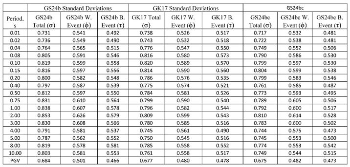
As discussed before, we are considering the 3rd dataset that includes 6045 data points, covering the range of moment magnitudes 4 ≤ ≤ 7.9 and rupture distances ≤ 250 km (M4_R250) to be the most important from the engineering applications point of view since it was created based on the recordings of earthquakes that can potentially produce damage. Figure 16 and Table 1 demonstrate the natural logarithmic standard deviation sigma () for the GS24b, GS24bc and GK17 model predictions applied to the 3rd dataset M4_R250. As expected, the newest GS24bc model demonstrates the lowest total sigma. However, previously developed GK17 sigma also demonstrates acceptable results.
We also split the total standard deviation () into within-event () and between-event () standard deviations.
The within-event standard error () is calculated by averaging within-event standard errors of earthquakes represented well enough in the database by more than 10 data points. Between-event standard deviation (τ) is calculated as
Table 1 shows total, within-event and between-event standard deviations of the models using the 3rd engineering dataset.
Figure 17, Figure 18 and Figure 19 demonstrate comparisons of the GS24b, GS24bc and GK17 ground motion models with empirical spectral accelerations data from the total M4_R400 dataset for the three magnitude ranges:
- 4.77 ≤ ≤ 5.21 with an average = 4.99
- 5.70 ≤ ≤ 6.24 with an average = 6.06
- 7.28 ≤ ≤ 7.9 with an average = 7.64.
The GK17 model’s sigma recommended for use in hazard calculations published in Graizer (2018, Table 1) is lower, having been developed using subset of data with ≥ 5.5 and ≤ 140 km following the practice of NGA-West2 GMM developers. For example, Campbell and Bozorgnia (2014) recommended using sigma for the subset of data with ≥ 5.5 and ≤ 80 km. We believe that it is more appropriate for engineering applications in seismic hazard calculations to use the 3rd subset of data shown in Figure 1 and Figure 2 for estimating sigma. Figure 16 also demonstrates sigma shown on the plot by a circle beyond the GMM range.
5. Results
The new GS24b backbone model is developed for the average RotD50 horizontal component of ground motion for shallow crustal earthquakes in active crustal regions. The model is derived based on a subset of the same NGA-West2 dataset [17] used in the development of the GK17 [14] model enhanced by the data from the three strong 2023 Turkish earthquakes with moment magnitudes 6.3, 7.5 and 7.8 with a total of 13926 data points [20]. We did not use data from earthquakes with moment magnitudes < 4.0 and limited the rupture distance range to 400 km. Records from earthquakes in Japan were also not used, because most of sites in Japan are characterized by subsurface geology significantly different from site conditions in other ACRs.
We consider the subset of 4 ≤ ≤ 7.9 and ≤ 250 km (M4_R250) of 6045 data points to be the most important from the engineering application point of view since it is limited to the data from earthquakes with magnitude-distance combinations that can potentially produce structural damage.
Similar to the GK17 [14], the new model has a bilinear attenuation slope of Rrup-1 representing geometrical spreading of body waves for the closest 50 km from the fault, and Rrup-0.5 at larger distances representing geometrical spreading of surface waves. The 50 km fault distance shift in the geometrical spreading is supported by the NGA-West2 data.
The number of input predictors in the GS24b model are limited to a few measurable parameters: moment magnitude , closest distance to fault rupture plane , time-averaged shear-wave velocity in the upper 30 m of the profile and apparent anelastic attenuation SA quality factor . This GS24b backbone GMM is applicable for earthquakes with 4.0 ≤ ≤ 8.5, at rupture distances from 0 < ≤ 400 km, at sites having 150 ≤ ≤1500 m/s, and for spectral periods of 0.01 ≤ ≤ 10 sec.
A distinctive feature of the GS24b global backbone model is that it uses the closed form approximation of the spectral acceleration as a multiplication of the and spectral shape functions. This model can be later used for adjusting to the specific active crustal region, for example, Southern or Northern California, Italy or Turkey creating region specific partially non-ergodic models, requiring only residual and apparent anelastic attenuation adjustment.
As an example, we created GS24bc model by adjusting the generic active crustal region backbone GS24b model for moment magnitude M, shear-wave velocity and fault rupture distance Rrup residuals using the NGA-West2 enhanced database. The GS24bc is an example of an easily created partially non-ergodic model demonstrating no residual biases. Compared to GK17 currently developed models also calculates PGV.
The previously developed GK17 [14] model tested against the engineering dataset M4_R250 demonstrated acceptable performance with standard error lower than the GS24b backbone model for periods T ≥ 0.1 s.
The GS24b and GS24bc ground motion models for spectral acceleration and peak ground velocity are developed using MATLAB software.
6. Data and Resources
The newly developed ground motion models discussed in this paper are based on the PEER Center Next Generation Attenuation Phase 2 (NGA-West2) database of processed ground motions from shallow crustal earthquakes in active tectonic regimes (http://ngawest2.berkeley.edu/). The NGA-West2 flatfile and the associated website were last accessed in July 2016. Turkish strong motion accelerometer data were retrieved from the Department of Earthquake, Disaster and Emergency Management Authority (AFAD; https://deprem.afad.gov.tr/stations) of Türkiye through the Turkish National Strong Motion Network (DOI: 10.7914/SN/TK), and Kandilli Observatory and Earthquake Engineering Research Institute of Boğaziçi University (KOERI, Istanbul; DOI: 10.7914/SN/KO) and processed by Buckreis et al. (2023a, 2023b) [18,19]. Other data used in this study came from the published sources listed in the text or in the references. All data processing was performed offline using a commercial software package (MATLAB R2024b, The MathWorks Inc., Natick, Massachusetts, 2024).
Author Contributions
Conceptualization, methodology and validation: V.G.; writing—original draft preparation, V.G. and S.S.; software: S.S and V.G. All authors have read and agreed to the current version of the manuscript.
Acknowledgments
We are grateful to Jonathan Stewart and Tristan Buckreis for providing access to the flatfiles of processed Turkey-Syria ground motion data. We thank Laurel Bauer for critical reviews, discussions and valuable comments that helped improving the quality of the manuscript. Previous joined work with Erol Kalkan resulted in the development of the original GK15 model serving as a foundation for creating updated GMMs.
Conflicts of Interest
The authors declare that they have no known competing financial interests or personal relationships that could have appeared to influence the work reported in this paper.
Disclaimer
Any opinions, findings and conclusions expressed in this paper are those of the authors and do not necessarily reflect the views of the United States Nuclear Regulatory Commission.
References
- Joyner, W. B., and Boore, D. M., 1993. Methods for regression analysis of strong-motion data, Bull. Seismol. Soc. Am. 83, 469–487. [CrossRef]
- Joyner, W. B., and Boore, D. M., 1994. Errata: Methods for regression analysis of strong-motion data, Bull. Seismol. Soc. Am. 84, 955–956. [CrossRef]
- Brillinger, D. R. and H. K. Preisler (1984). An exploratory analysis of the Joyner-Boore attenuation data, Bull. Seismol. Soc. Am. 74, 1441-1450.
- Brillinger, D. R. and H. K. Preisler (1985). Further analysis of the Joyner-Boore attenuationdata, Bull. Seismol. Soc. Am. 75, 611-614. [CrossRef]
- Abrahamson, N. A., and Youngs, R. R., 1992. A stable algorithm for regression analyses using the random effects model, Bull. Seismol. Soc. Am. 82, 505–510. [CrossRef]
- Abrahamson, N.A., Silva, W.J., and Kamai, R. (2014). Summary of the ASK14 Ground Motion Relation for Active Crustal Regions, Earthquake Spectra 30(3), 1025-1055. [CrossRef]
- Boore D. M., Stewart, J. P. Seyhan, E. and Atkinson, G. M. (2014). NGA-West2 Equations for Predicting PGA, PGV, and 5% Damped PSA for Shallow Crustal Earthquakes, Earthquake Spectra 30(3), 1057-1085. [CrossRef]
- Campbell, K.W., and Bozorgnia, Y. (2014). NGA-West2 Ground Motion Model for the Average Horizontal Components of PGA, PGV, and 5% Damped Linear Acceleration Response Spectra, Earthquake Spectra 30(3), 1087-1115. [CrossRef]
- Chiou, B., and Youngs, R.R. (2014). Update of the Chiou and Youngs NGA Model for the Average Horizontal Component of Peak Ground Motion and Response Spectra, Earthquake Spectra 30(3), 1117-1153. [CrossRef]
- Graizer, V. and Kalkan, E. (2007). Ground-motion attenuation model for peak horizontal acceleration from shallow crustal earthquakes, Earthquake Spectra, 23 (3), 585-613. [CrossRef]
- Graizer, V. and Kalkan, E. (2009). Prediction of response spectral acceleration ordinates based on PGA attenuation, Earthquake Spectra, 25 (1), 39-69.
- Graizer, V. and Kalkan, E. (2011). Modular filter-based approach to ground-motion attenuation modeling, Seismol. Res. Lett., 82, No. 1, 21-31. [CrossRef]
- Graizer, V. (2017). Alternative (G-16v2) Ground Motion Prediction Equations for Central and Eastern North America. Bull. Seismol. Soc. Am., 107, 869-886. [CrossRef]
- Graizer, V. (2018). GK17 Ground-Motion Prediction Equation for Horizontal PGA and 5% Damped PSA from Shallow Crustal Continental Earthquakes. Bull. Seismol. Soc. Am., 108, 380-398. [CrossRef]
- Wilson, H. B., Turcotte, H. L., and Halpern, D., 2003. Advanced Mathematics and Mechanics Applications Using MATLAB, 3rd edition, Chapman & Hall/CRC, Boca Raton, 696 p.
- Graizer, V. (2024). Application of GK17 Ground-Motion Model to Preliminary Processed Turkish Ground-Motion Recordings Dataset and GK Model Adjustment to the Turkish Environment by Developing Partially Nonergodic Model, Seismol. Res. Lett. 95, 651–663.17. [CrossRef]
- Ancheta, T. D., Darragh, R. B., Stewart, J. P., Seyhan, E., Silva, W. J., Chiou, B. S.-J., Wooddell, K. E., Graves, R. W., Kottke, A. R., Boore, D. M., Kishida, T., and Donahue, J. L. (2014). NGA-West2 database, Earthquake Spectra 30, 989–1005.
- Buckreis, T. E., B. Güryuva, A. İçen, O. Okcu, A. Altindal, M. F. Aydin, R. Pretell, A. Sandikkaya, O. Kale, A. Askan, S. J. Brandenberg, T. Kishida, S. Akkar, Y. Bozorgnia, J. Stewart. (2023a). Ground Motion Data from the 2023 Türkiye-Syria Earthquake Sequence. DesignSafe-CI. [CrossRef]
- Buckreis, T. E., B. Güryuva, A. İçen, O. Okcu, A. Altindal, M. F. Aydin, R. Pretell, A. Sandikkaya, O. Kale, A. Askan, S. J. Brandenberg, T. Kishida, S. Akkar, Y. Bozorgnia, J. Stewart. (2023b). February 6, 2023, Turkey earthquakes: Report on geoscience engineering impacts. Chapter 3. Ground Motions. https://10.18118/G6PM34 p.63-94.
- Graizer, V., Stovall, S., and Bauer, L. (2024). Global GS24 Ground Motion Models for Active Crustal Regions based on Non-Traditional Modeling Approach. Technical Letter Report [TLR-RES-DE-SGSEB-2024-01]. U.S. Nuclear Regulatory Commission. ADAMS ML24309A090 45 p.
- Boore, D. M. (2010). Orientation-independent, nongeometric-mean measures of seismic intensity from two horizontal components of motion, Bull. Seismol. Soc. Am. 100, 1830–1835. [CrossRef]
- Douglas, J. & Halldorsson, B. (2010). On the use of aftershocks when deriving ground-motion prediction equations. In 9th US National and 10th Canadian Conference on Earthquake Engineering (9USN/10CCEE), Paper no. 220, Toronto, Canada, 2010, 7456-7465.
- Idriss, I. M. (2013). NGA-West2 model for estimating average horizontal values of pseudo-absolute spectral accelerations generated by crustal earthquakes. Report PEER 20013/08, Pacific Earthquake Engineering Research Center, University of California, Berkeley, CA.
- Graizer, V. and Kalkan, E. (2016). Summary of the GK15 Ground-Motion Prediction Equation for Horizontal PGA and 5% Damped PSA from Shallow Crustal Continental Earthquakes. Bull. Seismol. Soc. Am., 106, 687-707. [CrossRef]
- Graizer, V. (2016). Ground-Motion Prediction Equations for Central and Eastern North America. Bull. Seismol. Soc. Am., 106, 1600-1612. [CrossRef]
- Graizer, V. (2022). Geometric spreading and apparent anelastic attenuation of response spectral accelerations. Soil Dynamics and Earthquake Engineering, 162, . [CrossRef]
- Idriss, I. M., and Sun, J. I., 1992. SHAKE91: a computer program for conducting equivalent linear seismic response analyses of horizontally layered soil deposits, Center for Geotechnical Modeling Department of Civil & Environmental Engineering, University of California, Davis.
- Kottke, A. R., and E. M. Rathje (2008). Technical manual for Strata, Report 2008/10, Pacific Earthquake Engineering Research (PEER) Center, Berkeley, California, 95 p.
- Gibbs, J. F., T. E. Fumal, D. M. Boore, and W. B. Joyner (1992). Seismic velocities and geological logs from borehole measurements at seven strong-motion stations that recorded the Loma Prieta earthquake, U.S. Geol. Surv. Open-File Rept. 92-287, Menlo Park, California, 139 p.
- De Alba P., R. L. Nigbor, J. H. Steidl, and J. C. Stepp (Editors) (2004). Proceedings of the International Workshop for Site Selection, Installation, and Operation of Geotechnical Strong-Motion Arrays, Los Angeles, California, COSMOS, 14 and 15 October 2004, 245 p.
- Kamai, R., Abrahamson, N. A., and Silva,W. J. (2014). Nonlinear horizontal site amplification for constraining the NGA-West2 GMPEs, Earthquake Spectra 30, 1223–1240. [CrossRef]
- Walling, M., Silva, W. J., and Abrahamson, N. A., (2008). Nonlinear site amplification factors for constraining the NGA models, Earthquake Spectra 24, 243–255. [CrossRef]
- Laurendeau, A., F. Cotton, O.-J. Ktenidou, L.-F. Bonilla, and F. Hollender (2013). Rock and stiff-soil site amplification: Dependencies on VS30 and kappa (κ0), Bull. Seismol. Soc. Am. 103, 3131–3148. [CrossRef]
- Ktenidou, O.-J., and N. Abrahamson (2016). Empirical estimation of high-frequency ground motion on hard rock, Seism. Res. Letters 87, 1465-1478. [CrossRef]
- Kishida, T., Haddadi, H, Darragh, R. B., Kayen, R. E., Silva, W. J., and Bozorgnia, Y. (2018). Apparent Wave Velocity and Site Amplification at the California Strong Motion Instrumentation Program Carquinez Bridge Geotechnical Arrays During the 2014 M6.0 South Napa Earthquake. Earthquake Spectra, 34, No. 1, 327–347. [CrossRef]
- Graizer, V. (2012). Effect of low-pass filtering and re-sampling on spectral and peak ground acceleration in strong-motion records. Proceedings of the 15 World Conference on Earthquake Engineering. Lisbon, Portugal 2012.
- Erickson, D., D. E. McNamara, and H. M. Benz (2004). Frequency-dependent Lg Q within the continental United States. Bull. Seism. Soc. Am., 94, 1630-1643.
- Malagnini, L., K. Mayeda, R. Urhammer, A. Akinci, and R. B. Herrmann (2007). A regional ground-motion excitation/attenuation model for the San Francisco region, Bull. Seismol. Soc. Am. 97, 843–862. [CrossRef]
- Mayeda, K., L. Malagnini, W. S. Phillips, W. R. Walter, and D. Dreger (2005). 2-D or not 2-D, that is the question: a northern California test, Geophys. Res. Lett. 32, L12301. [CrossRef]
- Ford, S.R., Dreger, D.S., Mayeda, K., Walter, W.R., Malagnini, L. and Philips, W.S. (2008). Regional attenuation in northern California; A comparison of five 1D Q methods, Bull. Seism. Soc. Am. 98(4) 2033–2046. [CrossRef]
- Chapman, M., and A. Conn (2016). A model for Lg propagation in the Gulf Coastal Plain of the southern United States, Bull. Seismol. Soc. Am. 106, doi: 10.1785/0120150197. [CrossRef]
- Morozov, I. B. (2008). Geometrical attenuation, frequency dependence of Q, and the absorption band problem. Geophys. J. Int. 175, 239–252.
- Booth, E. (2007). The Estimation of Peak Ground-motion Parameters from Spectral Ordinates, Journal of Earthquake Engineering, 11(1), 13-32. [CrossRef]
Figure 1.
Distribution of recordings with respect to moment magnitude and rupture distance (upper panel), peak ground acceleration () and (middle panel), and number of recordings in each subset depending upon maximum period range (lower panel). NGA-West2 data are shown with open circles and additional Turkish data with red circles.
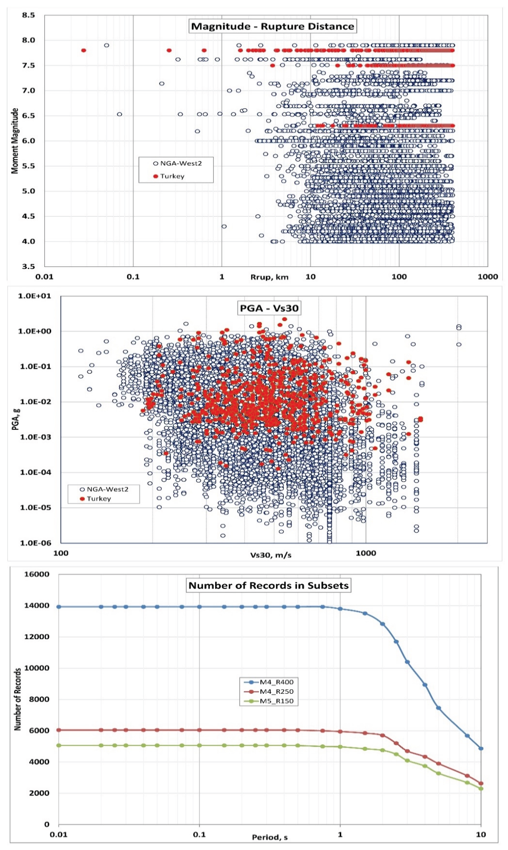
Figure 2.
The three datasets used to create GS24 GMMs.
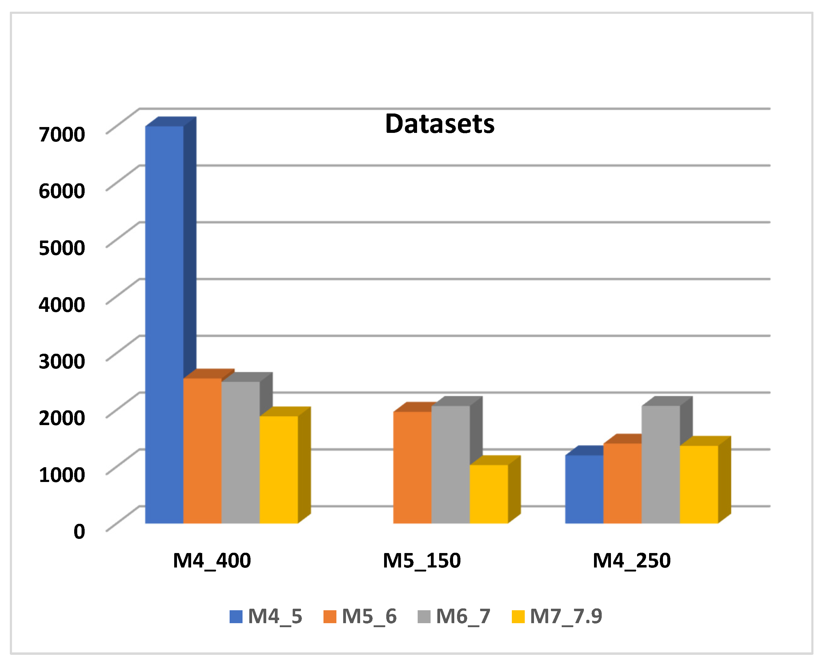
Figure 3.
magnitude scaling in GK17 and GS24.
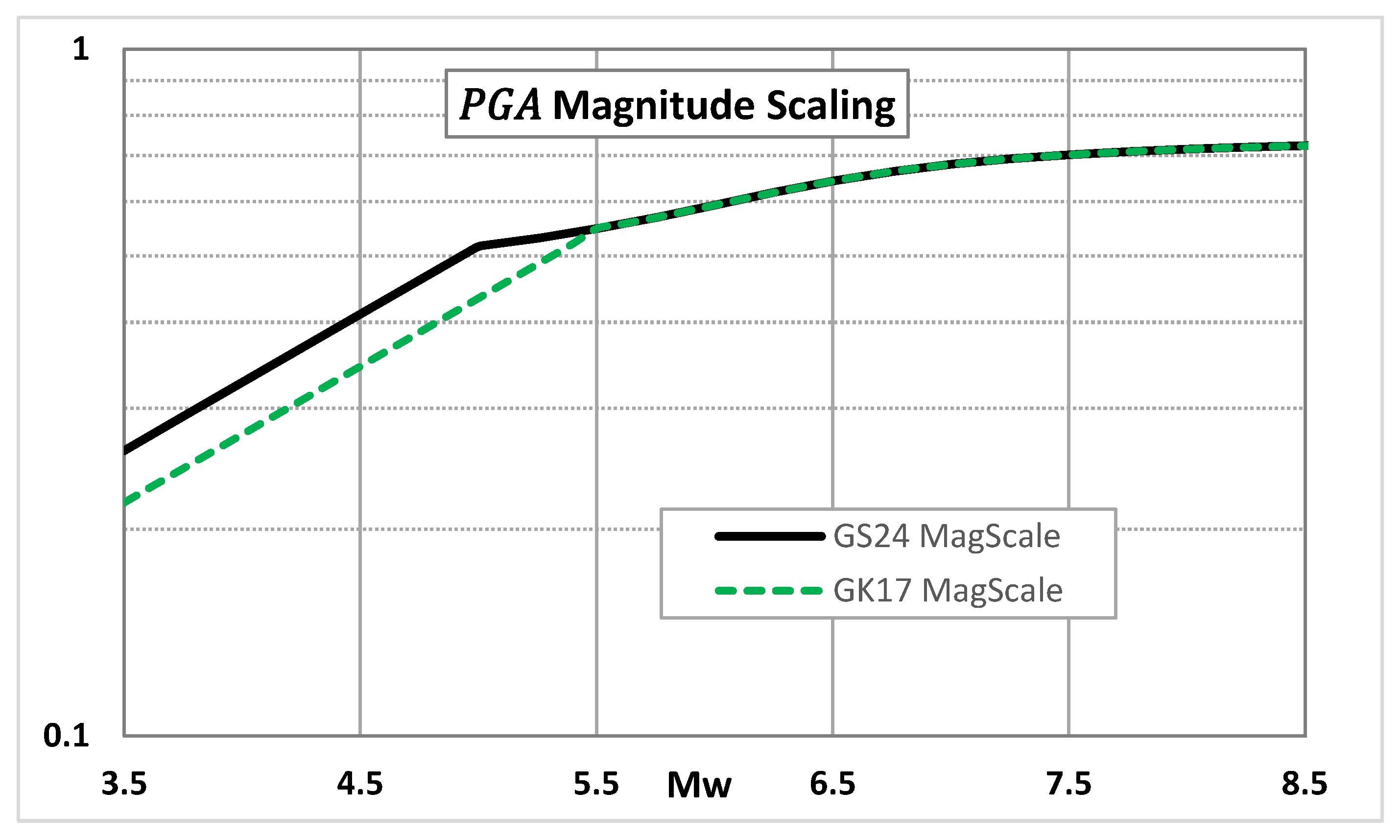
Figure 4.
Generic spectral shape model, and its controlling parameters: I(M,Rrup) - defines the peak spectral intensity, μ(M,Rrup) and Tsp,0(M,Rrup) define the predominant period of the spectrum, S(M,Rrup) - defines the wideness area under the spectral shape, and ζ - controls the decay of the spectrum at long periods (a). Spectral shape dependance on magnitude (b), rupture distance (c), and (d).
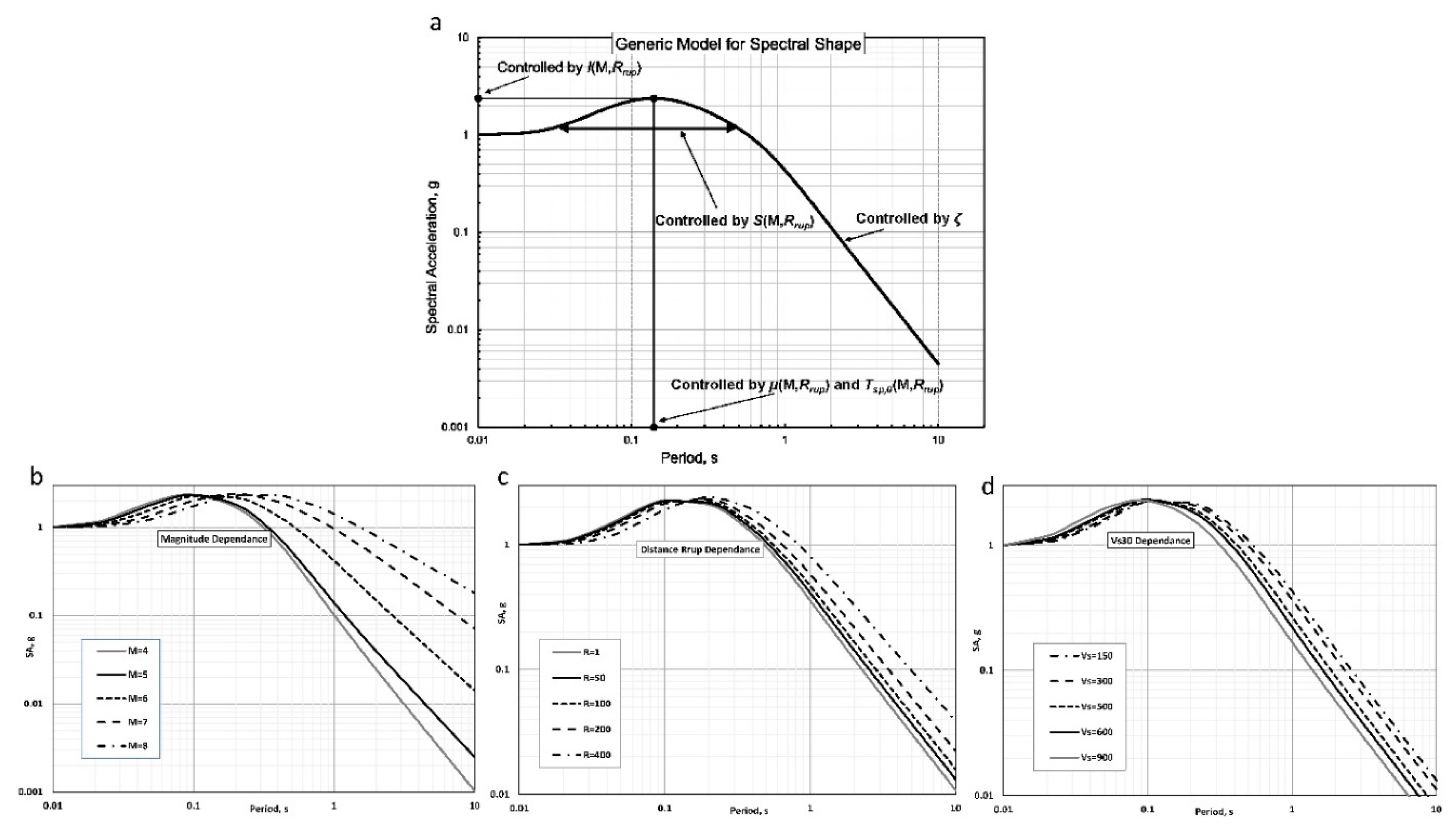
Figure 5.
G1 filter site amplification from Equation 8.
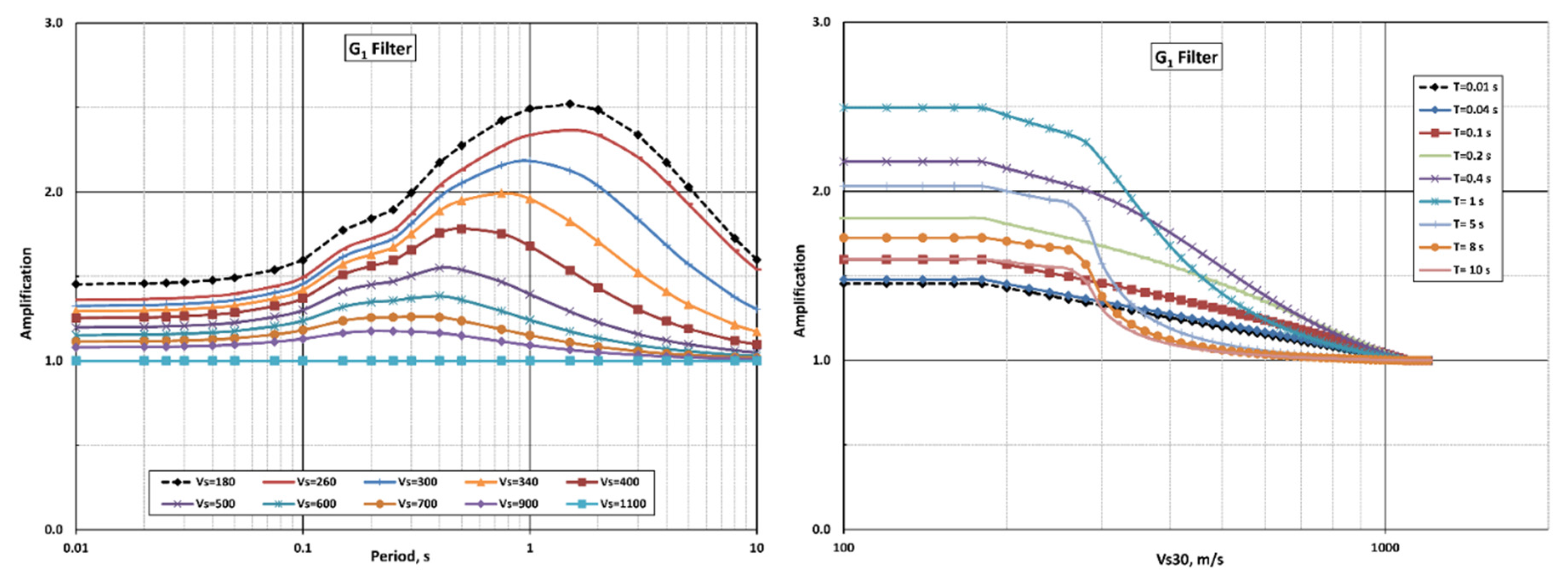
Figure 6.
Seismological and inverted with approximation by Equation 12.
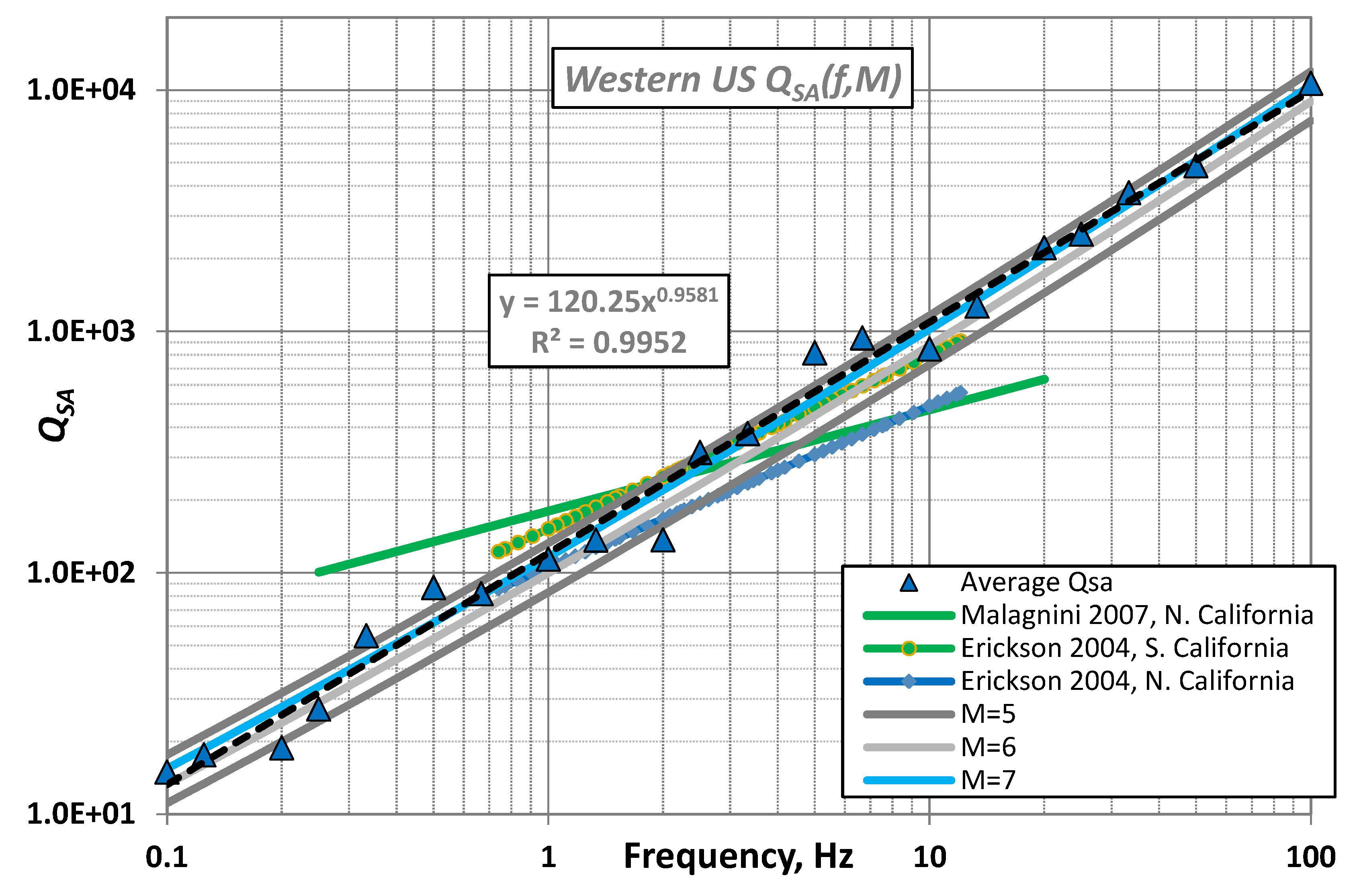
Figure 7.
Examples of response spectral accelerations at rupture distances of 10, 50 and 200 km for moment magnitudes varying from M=4.5 till 8 calculated using GS24b backbone model.
Figure 7.
Examples of response spectral accelerations at rupture distances of 10, 50 and 200 km for moment magnitudes varying from M=4.5 till 8 calculated using GS24b backbone model.
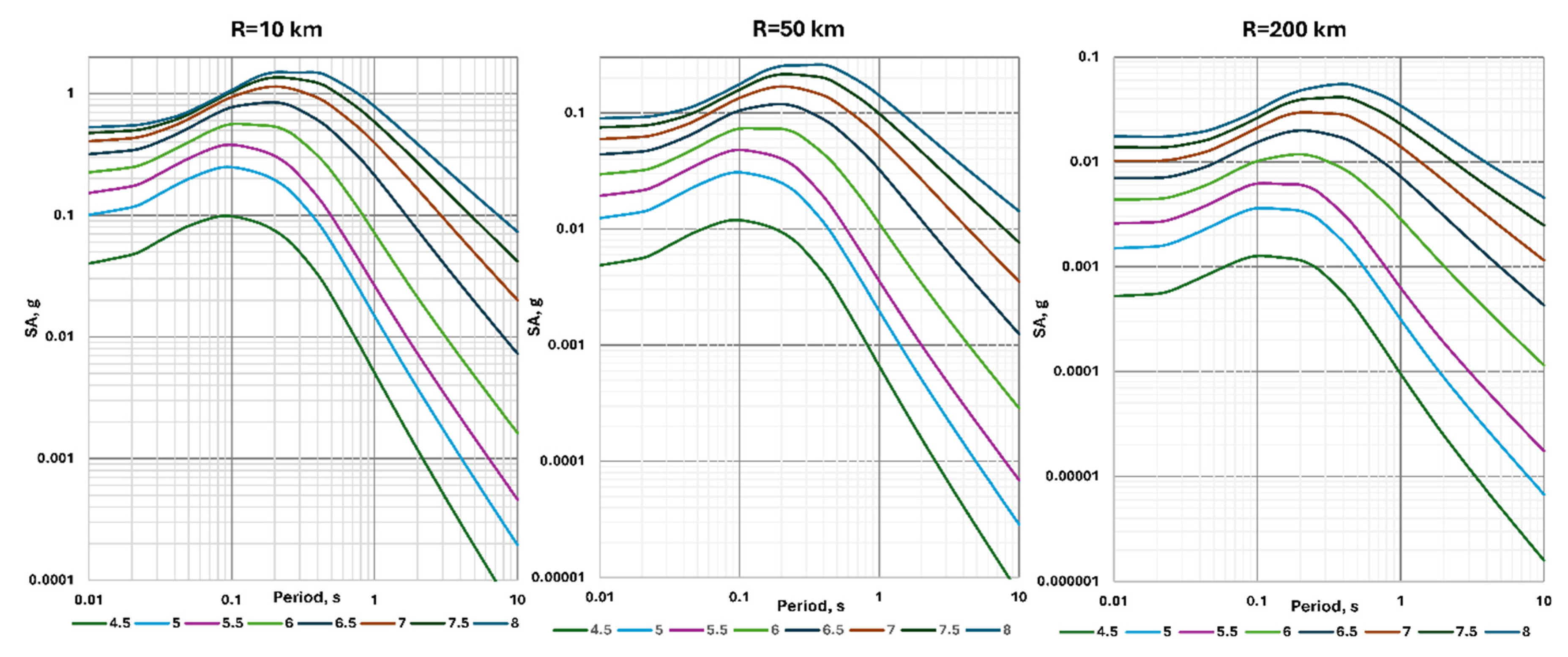
Figure 8.
Examples of different periods attenuation with distance to the fault for GS24b backbone model.
Figure 8.
Examples of different periods attenuation with distance to the fault for GS24b backbone model.
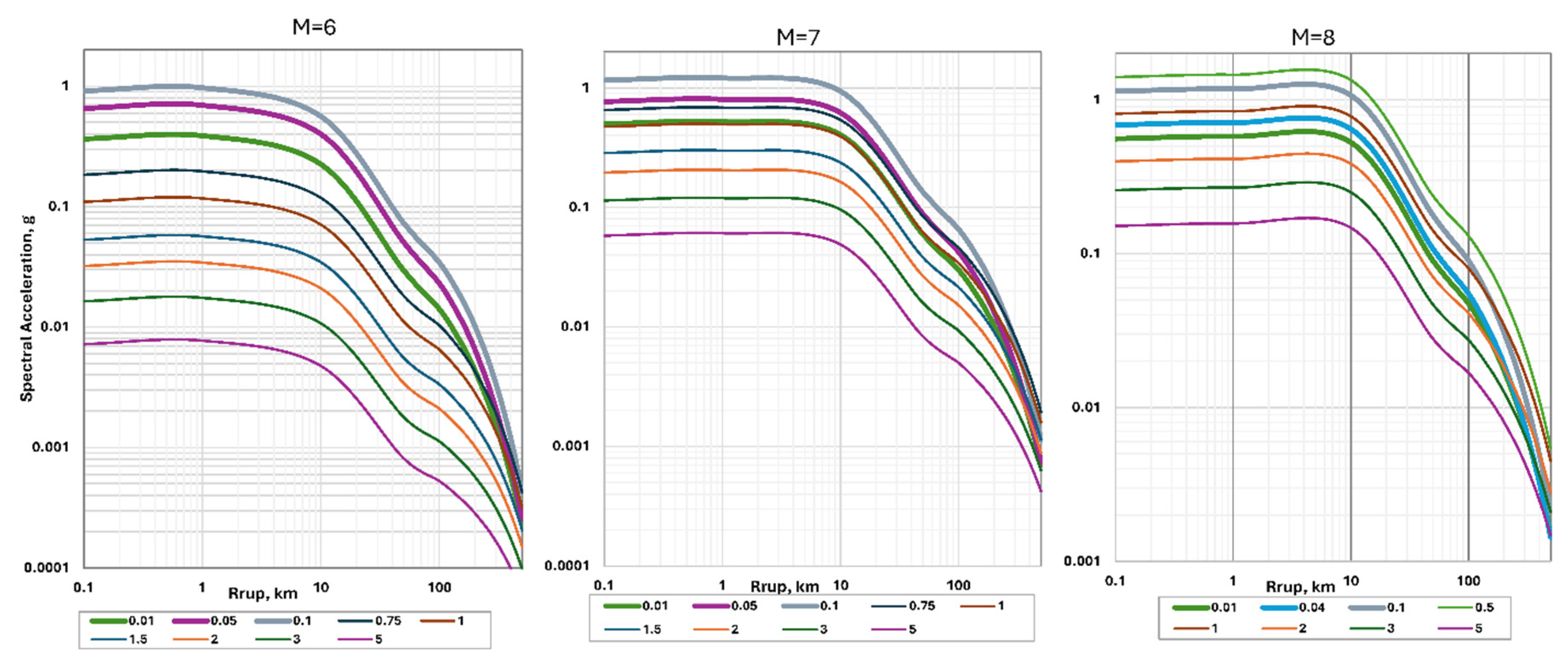
Figure 9.
Standard errors of GS24b and GK17 models predictions for the three subsets of data.
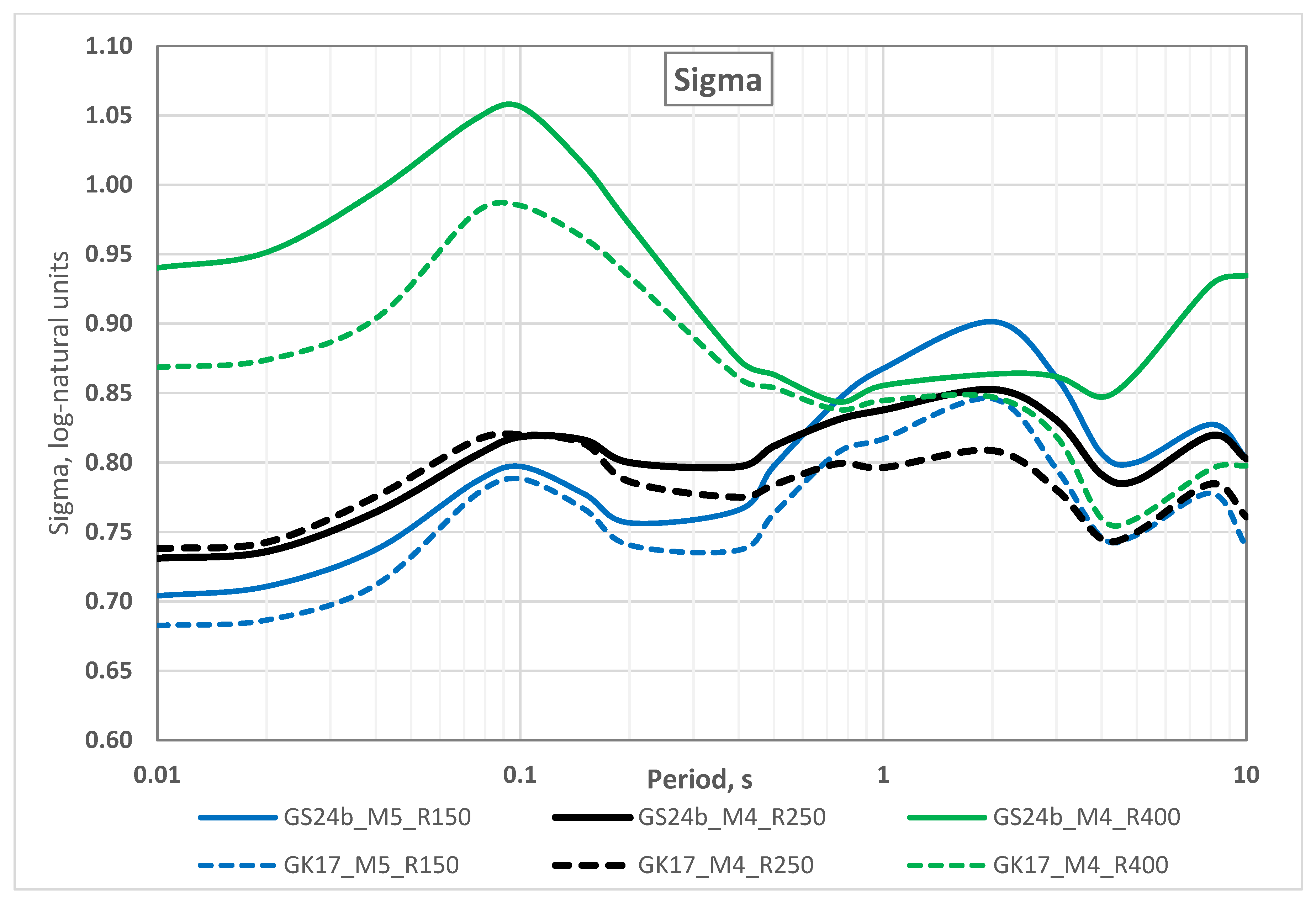
Figure 10.
GS24bc residuals versus moment magnitude M for frequencies of 100, 10, 1, and 0.33 Hz.
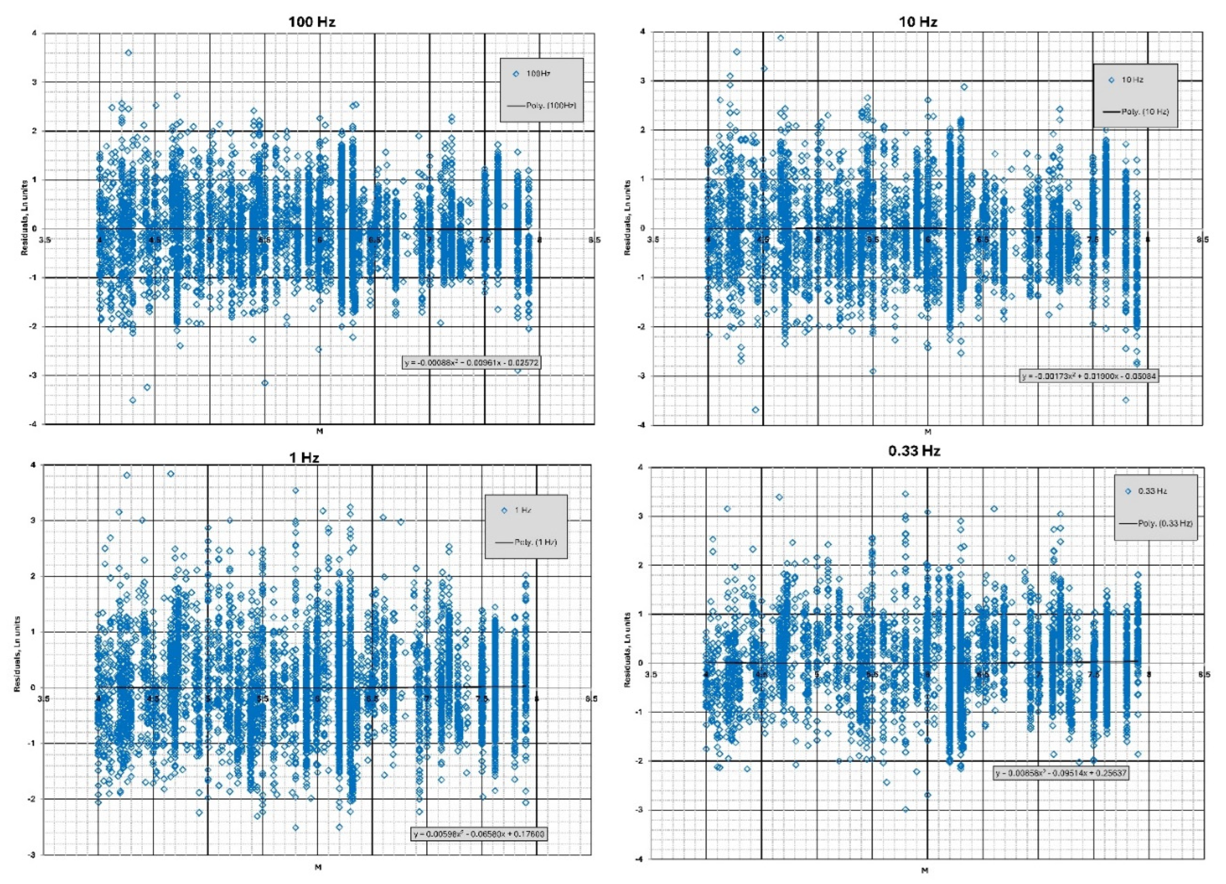
Figure 11.
GS24bc residuals versus Vs30 for frequencies of 100, 10, 1, and 0.33 Hz.
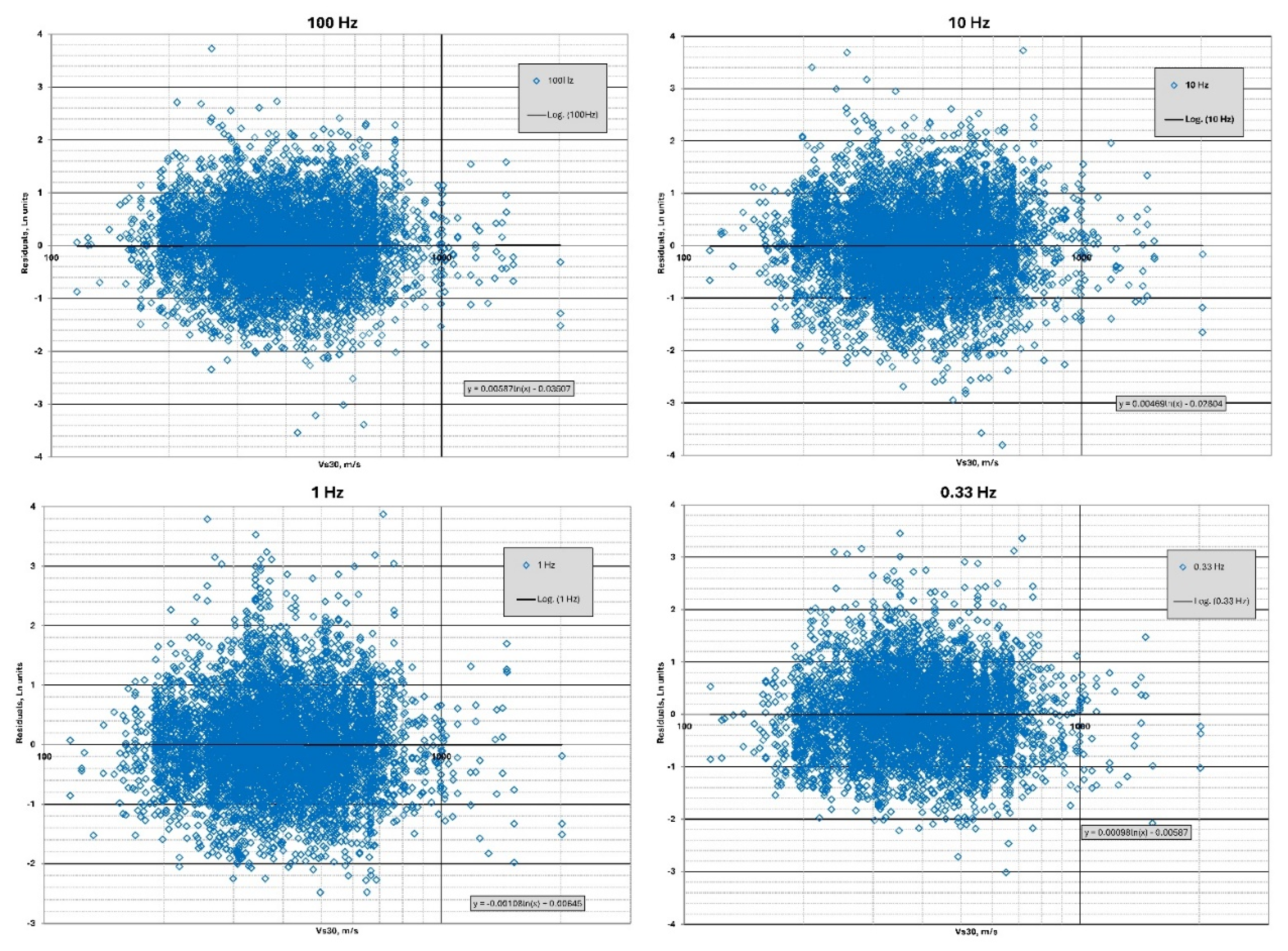
Figure 12.
GS24bc residuals versus fault rupture distance Rrup for frequencies of 100, 10, 1, and 0.33 Hz.
Figure 12.
GS24bc residuals versus fault rupture distance Rrup for frequencies of 100, 10, 1, and 0.33 Hz.

Figure 13.
GS24bc PGV residuals versus magnitude M, shear-wave velocity VS30 and fault rupture distance Rrup.
Figure 13.
GS24bc PGV residuals versus magnitude M, shear-wave velocity VS30 and fault rupture distance Rrup.
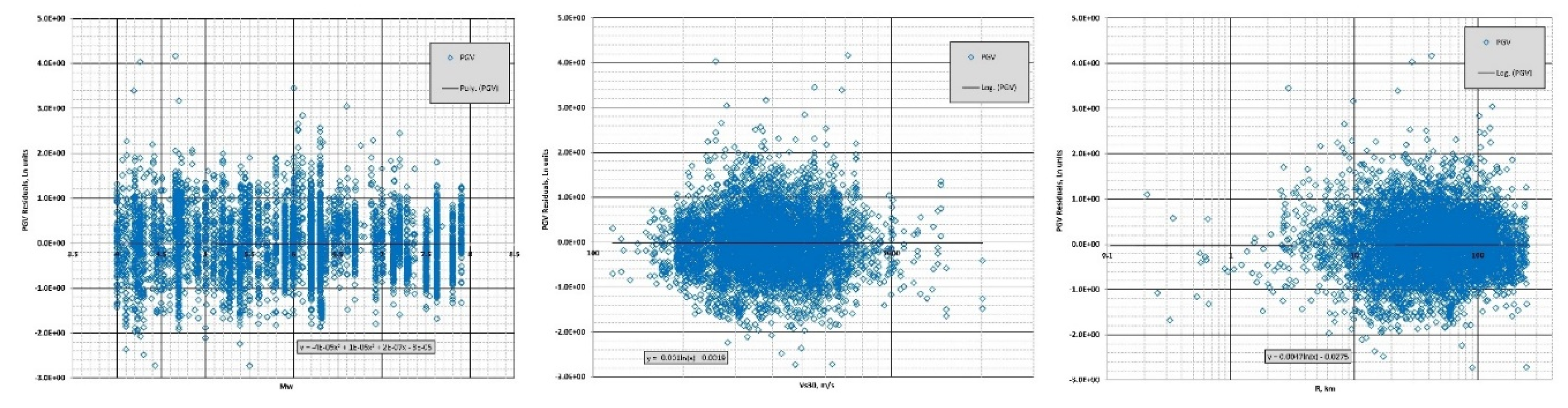
Figure 14.
Examples of response spectral accelerations at rupture distances of 10, 50 and 200 km for moment magnitudes varying from M=4.5 till 8 calculated using GS24bc model.
Figure 14.
Examples of response spectral accelerations at rupture distances of 10, 50 and 200 km for moment magnitudes varying from M=4.5 till 8 calculated using GS24bc model.
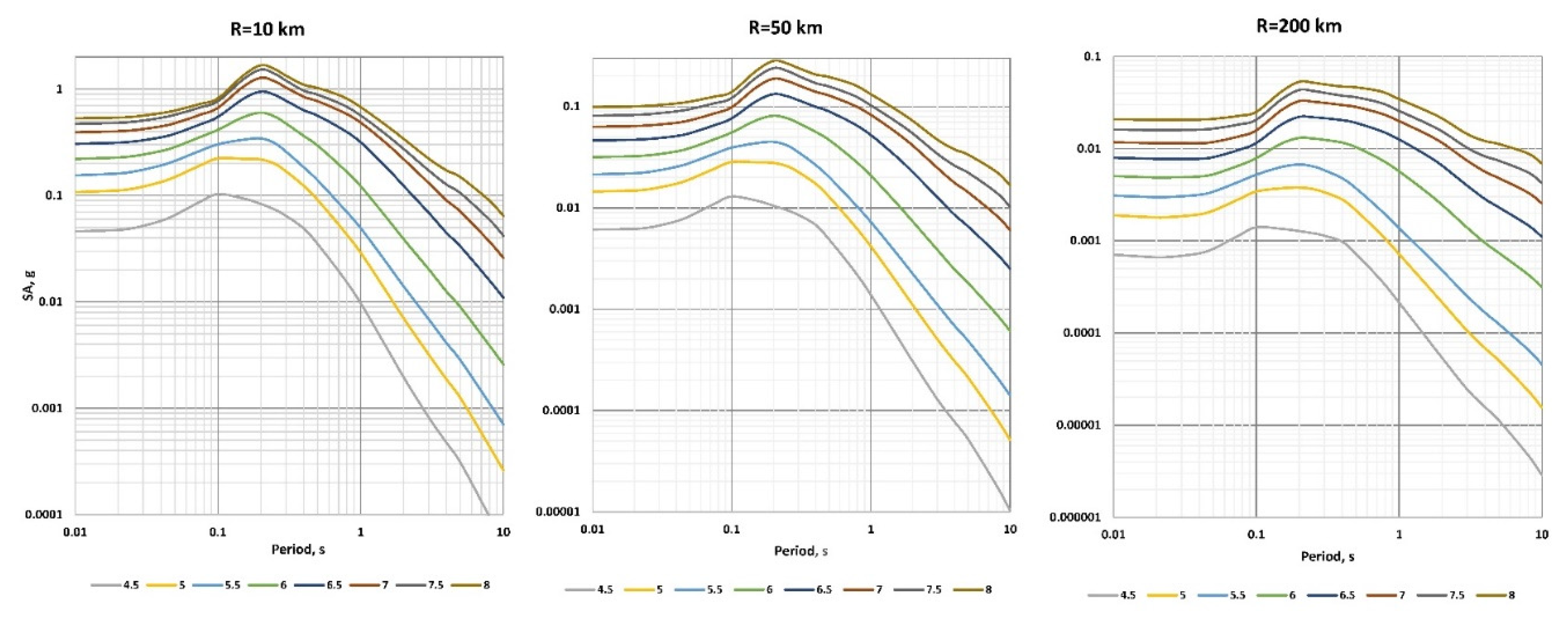
Figure 15.
Examples of different periods attenuation with closest distance to the fault for the GS24bc model.
Figure 15.
Examples of different periods attenuation with closest distance to the fault for the GS24bc model.
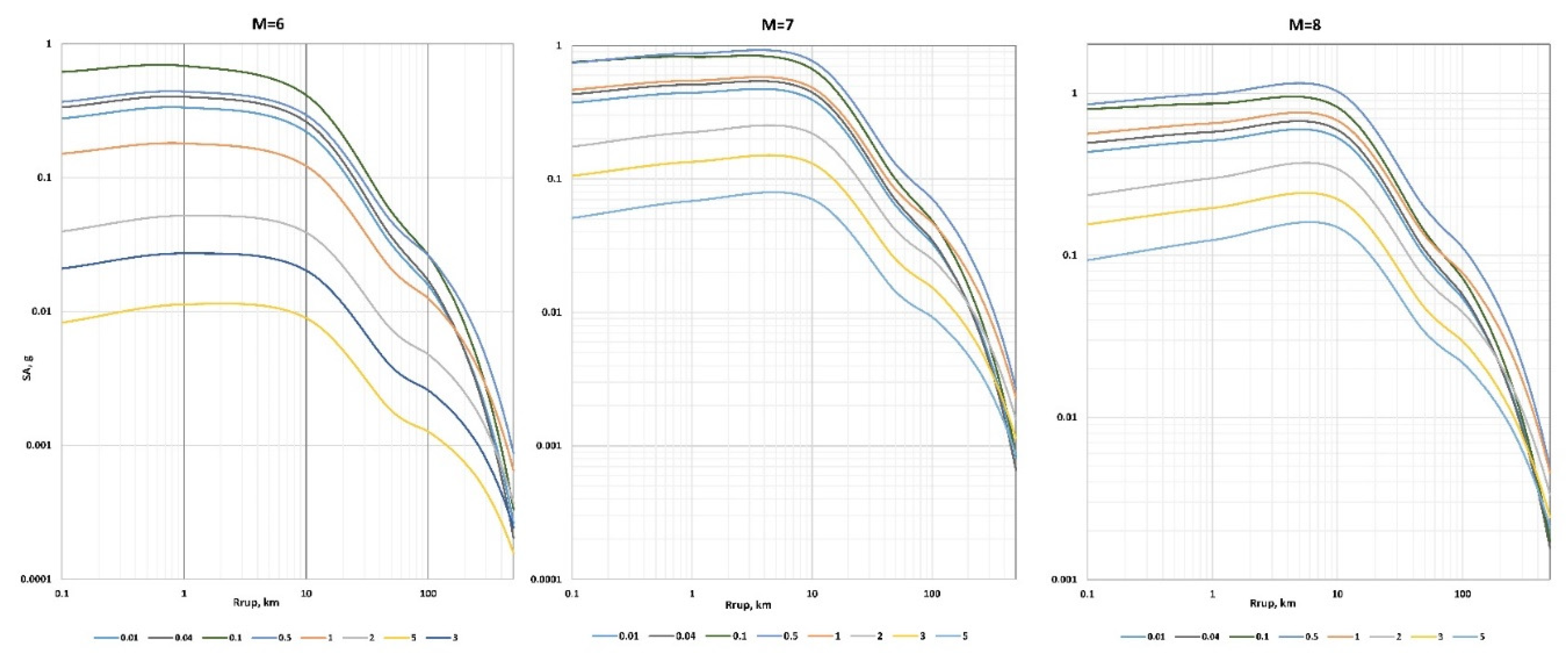
Figure 16.
Natural logarithmic standard deviation sigma () for the GS24b, GS24bc and GK17 model predictions for the 3rd dataset M4_R250.
Figure 16.
Natural logarithmic standard deviation sigma () for the GS24b, GS24bc and GK17 model predictions for the 3rd dataset M4_R250.
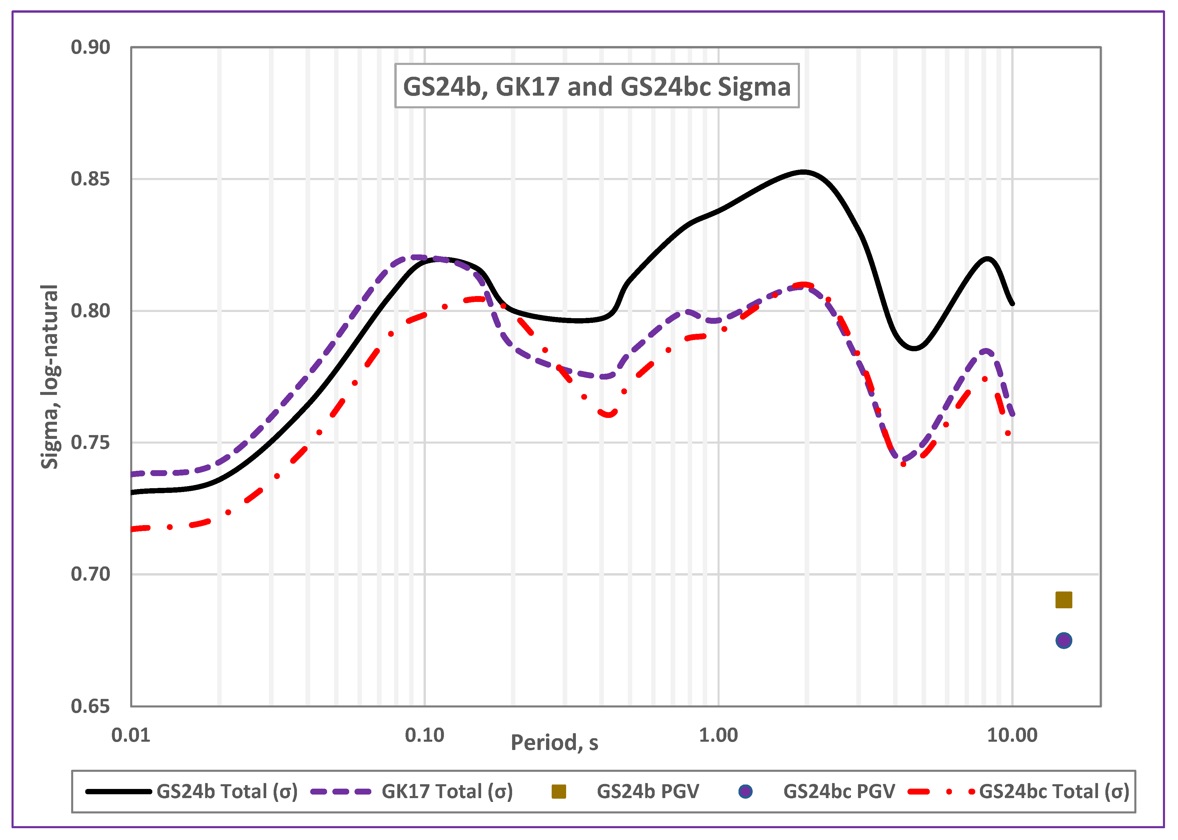
Figure 17.
Comparison of the recorded spectral accelerations (open circles) from earthquakes in a magnitude range of 4.77 to 5.21 and calculated using the GS24b, GS24bc and GK17 ground motion models SA for the average earthquake of M = 4.99 and average Vs30 = 456 m/s.
Figure 17.
Comparison of the recorded spectral accelerations (open circles) from earthquakes in a magnitude range of 4.77 to 5.21 and calculated using the GS24b, GS24bc and GK17 ground motion models SA for the average earthquake of M = 4.99 and average Vs30 = 456 m/s.
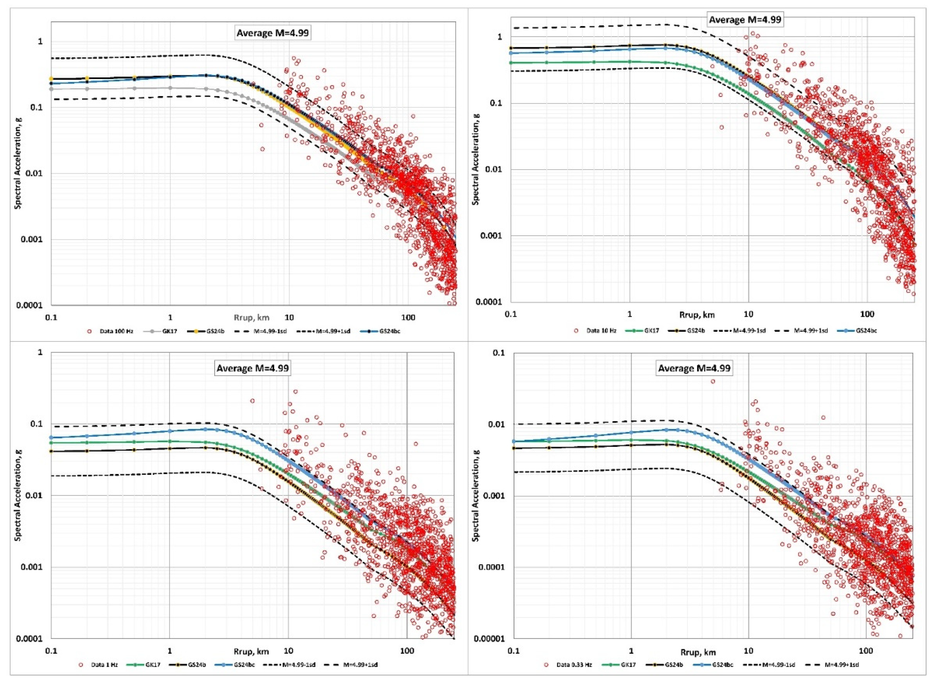
Figure 18.
Comparison of the recorded spectral accelerations (open circles) from earthquakes in a magnitude range of 5.7 to 6.24 and calculated using the GS24b, GS24bc and GK17 ground motion models SA for the average earthquake of M = 6.06 and average Vs30 = 414 m/s.
Figure 18.
Comparison of the recorded spectral accelerations (open circles) from earthquakes in a magnitude range of 5.7 to 6.24 and calculated using the GS24b, GS24bc and GK17 ground motion models SA for the average earthquake of M = 6.06 and average Vs30 = 414 m/s.
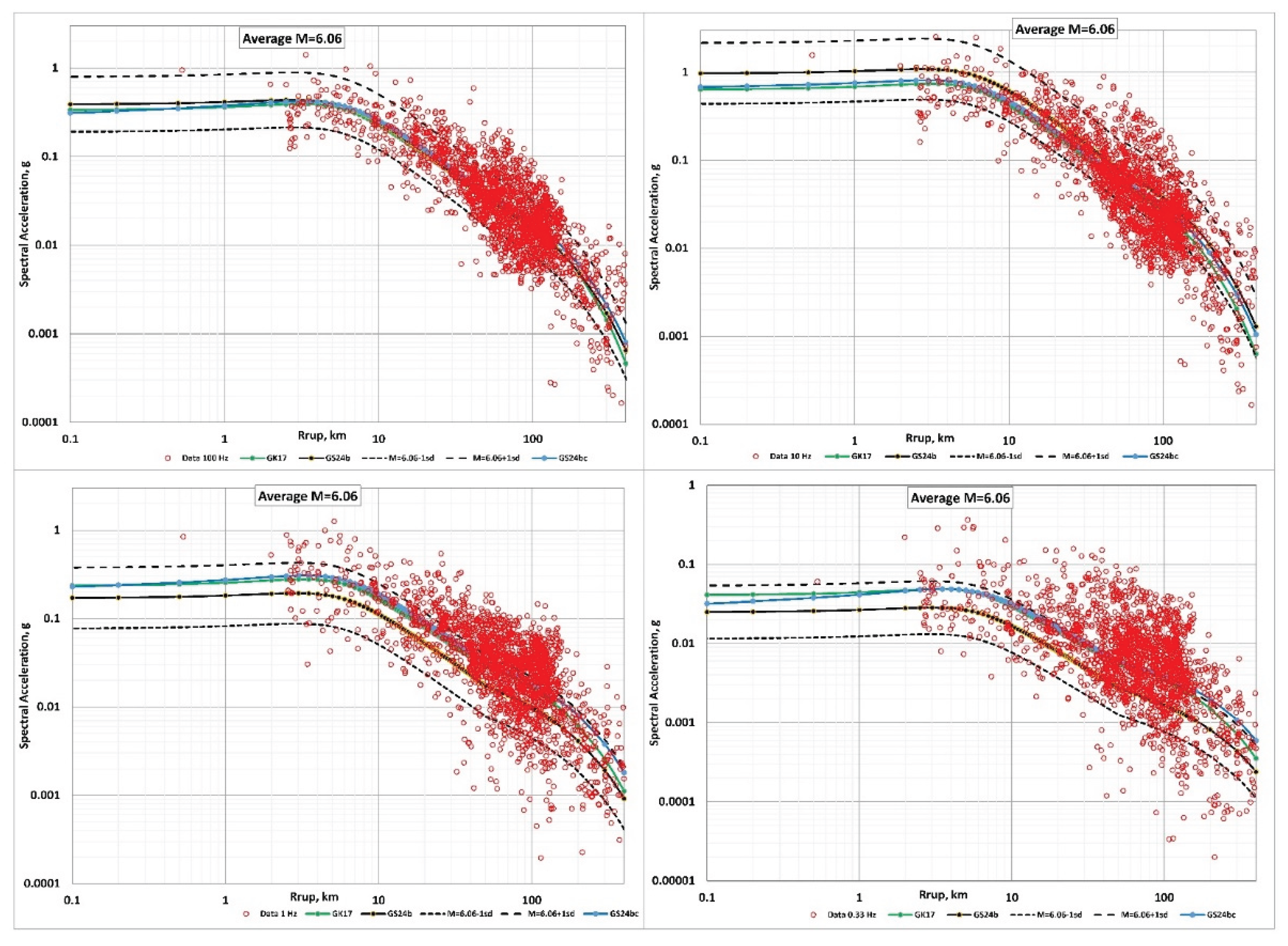
Figure 19.
Comparison of the recorded spectral accelerations (open circles) from earthquakes in a magnitude range of 7.28 to 7.9 and calculated using the GS24b, GS24bc and GK17 ground motion models SA for the average earthquake of M = 7.64 and average Vs30 = 451 m/s.
Figure 19.
Comparison of the recorded spectral accelerations (open circles) from earthquakes in a magnitude range of 7.28 to 7.9 and calculated using the GS24b, GS24bc and GK17 ground motion models SA for the average earthquake of M = 7.64 and average Vs30 = 451 m/s.
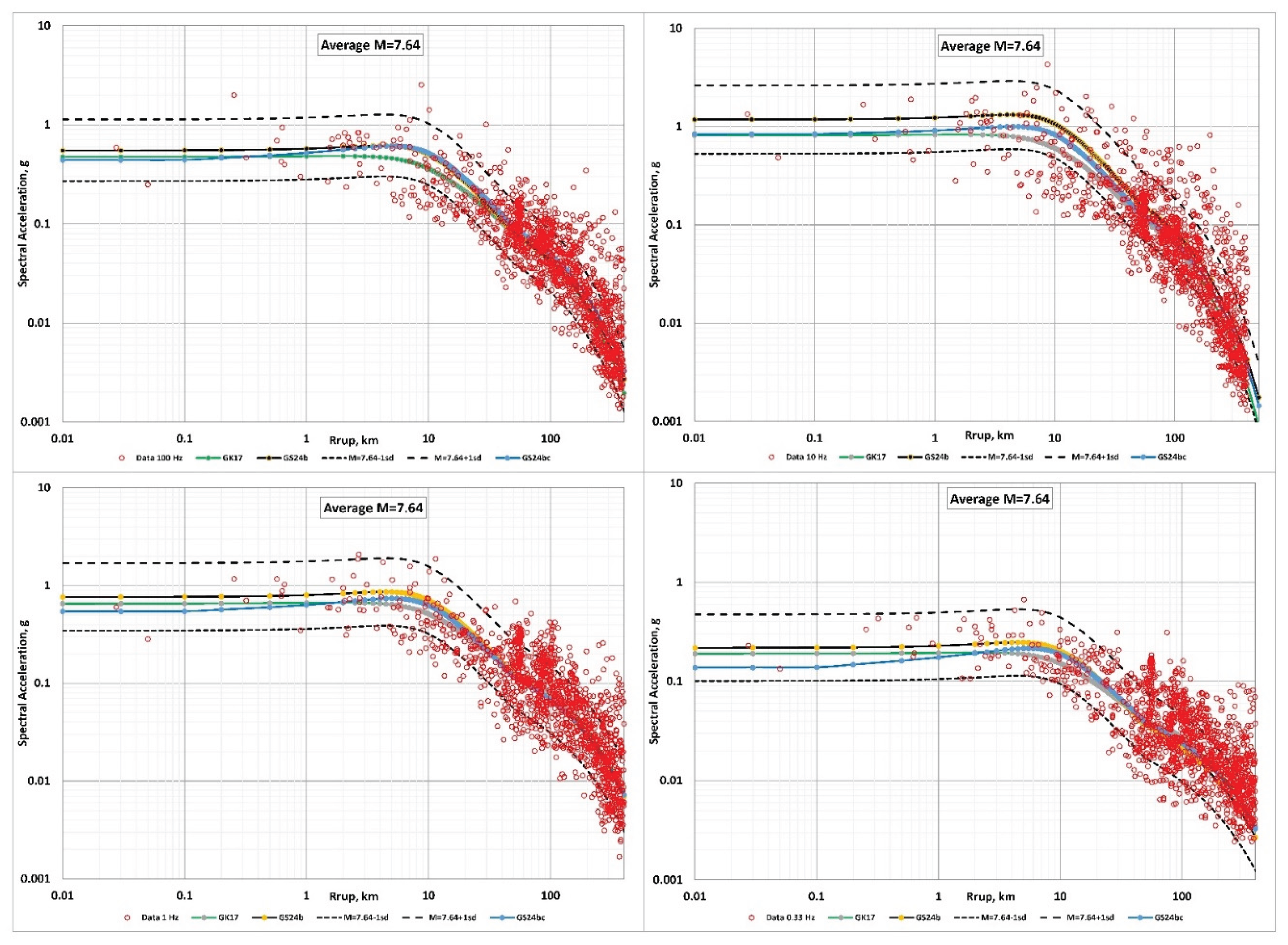

Table 1.
Sigma.
Disclaimer/Publisher’s Note: The statements, opinions and data contained in all publications are solely those of the individual author(s) and contributor(s) and not of MDPI and/or the editor(s). MDPI and/or the editor(s) disclaim responsibility for any injury to people or property resulting from any ideas, methods, instructions or products referred to in the content. |
© 2025 by the authors. Licensee MDPI, Basel, Switzerland. This article is an open access article distributed under the terms and conditions of the Creative Commons Attribution (CC BY) license (http://creativecommons.org/licenses/by/4.0/).
Copyright: This open access article is published under a Creative Commons CC BY 4.0 license, which permit the free download, distribution, and reuse, provided that the author and preprint are cited in any reuse.


