Submitted:
29 May 2025
Posted:
30 May 2025
Read the latest preprint version here
Abstract
The last few years have seen an increase in the amount of data collected in Structural Health Monitoring (SHM) systems. This can be attributed to the availability of cheap sensors and means of data transmission. However, this increase in data presents a challenge in meaningful analysis. Recently, practitioners and researchers have turned to deep learning methods for analysis of such data. Deep learning has already proven to be effective at analysing complex, highly dimensional datasets and this suits well with SHM data streams. The common data type in SHM is time series and mostly comes from vibration based SHM. Unlike static data, time series usually depict temporal dependencies and contextual variations. Further to this, time series are usually noisy and contain missing values. These attributes make the analysis of time series more complex. In deep learning, time series analysis is tackled using specialized architectures such as recurrent neural networks or through careful feature engineering. Considering these issues, it is important to understand the deep intricacies of these models for their effective application and development of new robust models.So far, different reviews have been conducted to provide a state of the art status of deep learning in SHM. However, it is clear that most of the reviews are usually application-centric and rarely consider a deep technical discussion of deep learning analysis for time series. Again, issues to do with uncertainty quantification and data augmentation are rarely discussed from a theoretical standpoint. This review seeks to tackle these issues and provide a deep theoretical review of time series, typical applications, and challenges. The goal is basically to provide the necessary background for researchers and practitioners in SHM to develop new models and to effectively apply the existing models to time series problems.
Keywords:
Time series
; Deep learning
; Structural Health Monitoring
1. Introduction
Many civil infrastructures are in a poor state [1,2,3]. This is mainly due to poor maintenance practices as well as exposure of the infrastructure to harsh environmental conditions [4]. Besides these, structural deterioration has been associated with misuse of infrastructure [5]. Regardless of the cause, structures in such a state usually pose risk to life, property and economic performance. Talking of negative impacts of structural deterioration, South Africa is a good example. To put this into context, South Africa loses almost 50% of the water pumped into its piped networks to leakages, among other factors [6]. This is in part due to deteriorating infrastructure which is rarely maintained. Problems related to deteriorating infrastructure are also encountered in South Africa’s power sector and transportation system [2]. The issue of deteriorating structures is further highlighted in South Africa’s Infrastructure Development scenarios for 2050 [7]. While the problem of deteriorating infrastructure is worse in the developing world, similar challenges are also observed in developed countries. A recent report by MakeUK indicates that approximately 54% of manufacturers in the United Kingdom perceive a decrease in road infrastructure quality over the last decade [8]. These statistics are a clear indication that interventions have to be taken to ensure serviceability of the existing infrastructure. Considering the economic value of civil infrastructure, their exposure to harsh environmental influences, and progressive material deterioration, conventional inspection and maintenance practices, which often rely on manual and periodic interventions, are insufficient to ensure structural integrity and long-term serviceability. As such, there is a need for continuous monitoring to enable early detection of deterioration and timely maintenance decisions [9,10].
Structure Health Monitoring (SHM) appears to be a promising solution to the issues discussed. The field of SHM was developed in the 1990s and has since matured over the years [11]. These days, SHM is extensively studied and applied to civil infrastructure. The aim of SHM is to enable damage identification, localisation, quantification and prognosis. This is accomplished through instrumentation, whereby sensors are deployed to collect data from a structure, followed by data analysis. Fundamentally, SHM is guided by 7 Axioms [12]. Of particular interest to this review is Axiom IV(a), which states that sensors cannot measure damage as such feature extraction is necessary to convert sensor data to damage information. In this regard, statistical and deep learning methods are used.
SHM involves the deployment of permanently installed sensors on a structure to gather data related to structural response and environmental conditions [13]. Collected data may include vibration signals, strain histories, humidity, among others. Despite the role of sensors in data collection, axiom IV(a) states that sensors cannot measure damage as such feature extraction is necessary to convert sensor data to damage information. In this regard, statistical and deep learning methods are used.
SHM methods are usually classified into two main categories: global and local [14]. Global methods typically involve acquisition of data across a full structure. The data is then processed to assess damage. Vibration based SHM methods fall under this category. Global methods can be used to detect, locate, and quantify damage on a structure. On the other hand, local methods focus on a particular area of a structure. In most cases, the location is known a priori and the goal is to assess the level of damage. Some methods under non-destructive evaluation are in this category. Considering the wide availability of cheap sensors, modern SHM systems are hugely global and a common characteristic of such methods is that the generated data is time series. It is therefore important that time series analysis is well understood.
Traditionally, time series analysis uses methods such as Auto Regressive Moving Average(ARMA), AutoRegressive Moving Average with eXogenous excitation (ARMAX), and state space models (SSMs), among others [6]. This is so because time series data exhibit correlations and dependencies which are otherwise absent in static data. Despite the successes of these methods on SHM systems, current data scale in SHM makes them inefficient in some cases. These traditional methods require assumptions which do not fit reality. As is the case with real world systems, noise and missing data are a common issue. Furthermore, modern SHM systems generate huge amounts of highly dimensional data and traditional methods have always found it difficult to analyse such data due to a phenomenon called the curse of dimensionality.
Recently, researchers have turned to deep learning to resolve these issues. Deep learning has proven to work extremely well in high dimensional spaces. With regards to time series, deep learning methods designed for sequential modeling have proven to be effective [15]. However, despite this, the application of deep learning to time series in SHM proves to be an outstanding issues for a number of reasons. Firstly, despite the generation of huge amounts of data by SHM systems, most of this data is inconsistent, contain significant amount of noise and is unlabeled. Secondly, in the real world, the accuracy of models is significantly poor which among other issues is due to domain shift. This is the case because structures are exposed to extremely harsh environments whose nuances might have not been captured in the model. A highlight on these issues is also the lack of integration of existing knowledge in developed models. Another issue with deep learning models is their high computational costs which hinders their development and deployment [16]. Deep learning models are known to be computationally demanding due to the enormous matrix operations which are performed during training and inference. A fourth and less commonly considered reality are regulatory restriction. The advent of tools like ChatGPT have brought this issue to light [17]. As for structural systems, which by the end of the day can impact life and economies, their deployment is trivial. This is a serious issue as classical deep learning is inherently deterministic and black-box, in which case no rationale is provided for the decision made by the system.
The aim of this paper is therefore to provide a mathematically grounded review of deep learning for time series in an attempt to address the current challenges and scepticisms. The review provides a discussion of neural network architectures which are common in time series, generative deep learning models, and uncertainty quantification in deep learning.To ensure the review is self-contained, we include derivations of key results where appropriate.Although the first part of this review tackles deep learning in general, the primary target audience of this review are SHM practitioners and researchers. Thus, the review provides a discussion of deep learning for time series in SHM, including challenges.
The remainder of the paper is structured as follows: It begins with the discussion of the related works in Section 2. To provide context, Section 3 provides the background to deep learning. This is followed by a discussion of generative models in Section 5. A review of uncertainty quantification in deep learning is provided in Section 6 .The final discussion in this review deals with applications in Section 7, state of DL in SHM in Section 8 and a concluding synthesis in Section 9
2. Related Works
In recent years, deep learning (DL) has gained significant traction in structural health monitoring (SHM) due to its ability to model complex, high-dimensional, and often nonlinear data [18,19]. Since 2020, several review studies have emerged to synthesize the expanding range of DL applications in SHM. This section analyzes 24 key publications that collectively reflect the current state of research, with a focus on methodological trends and persistent research gaps.
Several reviews have aimed to map the application of DL in SHM. Jia and Li [20], for example, presented a taxonomy based on data types, emphasizing the prevalence of vibration- and vision-based methods. However, their review lacked systematic coverage of sequential modeling or generative approaches. Similarly, Afshar et al. [21] emphasized the predictive power of neural networks for the prediction of structural responses, but provided minimal theoretical grounding.
A focused subset of the current literature addresses vibration-based SHM. Notable among these are works by Spencer et al. [18], Toh and Park [22], Azimi et al. [23], Indhu et al. [24], Wang et al. [25] and Avci et al. [26]. While insightful regarding modal data, these reviews largely overlooked temporal models such as recurrent neural networks (RNNs), temporal convolutional neural networks (TCNNs), and long short-term memory networks (LSTMs), resulting in an application-centric rather than theory-driven perspective.
In vision-based SHM, studies by Hamishebahar et al. [27], Chowdhury and Kaiser [28], Gomez-Cabrera and Escamilla-Ambrosio [29], Sony et al. [30] and Deng et al. [31] reviewed CNN-based methods for surface crack detection, defect classification , among others. Though these works offered comprehensive discussions of image-based SHM and relevant architectures, they paid little attention to temporal modeling, hybrid strategies, or generalization beyond specific materials. Chowdhury and Kaiser [28], for example, focused solely on concrete structures.
A few studies have attempted a more integrative approach. Khan et al. [32] explored hybrid methods combining DL with physics-based models, identifying avenues for methodological convergence, but their review lacked coverage of generative models and uncertainty quantification. Zhang et al. [33] focused on DL-based imputation techniques for incomplete SHM data, though without a rigorous theoretical foundation for the models used.
Despite the rising interest in generative models, only Luleci and Catbas [34] and Luleci et al. [35] have examined their use in SHM, and both lacked mathematical depth. Other reviews by Spencer et al. [18], Cha et al. [36], Abedi et al. [37], Zhang et al. [38], Tapeh and Naser [39] and Xu et al. [40] have made notable contributions, yet often remained narrowly application-focused and did not thoroughly address the theoretical principles underlying DL models.
Collectively, several limitations emerge across the current reviews. Most reviews remain confined to either vision-based or vibration-based SHM, with little integration of multimodal approaches or comparative learning paradigms. While CNNs are extensively covered, sequential models such as LSTMs, gated recurrent units (GRUs), and attention-based architectures receive insufficient attention, despite their common usage in SHM.This analysis finds no prior review dedicated exclusively to these models. Generative models are rarely discussed in depth, and theoretical treatments of uncertainty quantification are largely absent.
CNNs continue to dominate existing literature, while key areas such as uncertainty quantification and generative modeling are rarely covered, and when they are, theoretical treatment is minimal. This review addresses these gaps by providing a unified synthesis of deep learning methods, grounded in theory and explicitly tied to SHM applications. While some theory-focused or theory-practice-focused reviews exist, such as those on RNNs [15], generative models [41], time series [42,43,44], and uncertainty quantification [45,46],this work stands out by offering an integrated perspective across multiple DL paradigms. To the best of our knowledge, it is the first to do so.
3. Background
3.1. Time Series
Since Structural Health Monitoring (SHM) involves continuous monitoring of structures, a significant portion of the generated data is time series [47]. This data may include accelerometers, strain gauges, displacement transducers, and piezoelectric elements that capture the structural response to operational and environmental loading [13] . SHM data is often multivariate, noisy and might contain missing values. As such, modeling this data requires taking these issues into consideration.
Formally, a time series can be represented as where denotes the number of dimensions and L represents the length of the time series [43].
Time series are grouped into two major categories, i.e. univariate and multivariate. In a univariate time series, D=1. A typical example would be water level in a dam. For a multivariate time series, D> 1, and thus additional variables are considered. The presence of multiple variables introduces complexity as they may exhibit correlations which need to be taken into account during analysis. In the dam context, water levels are most likely influenced by daily temperature fluctuations and seasonal variations in rainfall.
Time series models typically serve four key purposes, namely; classification [48], forecasting[49], anomaly detection [50,51], and data imputation [52]. In an SHM system, classification involves assigning labels to time series data based on patterns identified in structural behaviour. A common classification task might be the categorization of the state of a structure based on inspection records. On the other hand, forecasting deals with the prediction of future values based on historical trends. In most cases, forecasting deals with continuous values and provides a quantitative outlook on how a system is likely to evolve over time. Anomaly detection (Figure 1) plays a crucial role in identifying deviations from normal behaviour that may indicate a number of issues such as structural damage, shock events e.g. an earthquake, sensor malfunction or simply false alarms. This is important to ensure that events are correctly detected and an appropriate action is taken. Most importantly, anomaly detection can help save a structure and life of its users or occupants.Finally, data imputation focuses on estimating and filling in missing values to ensure the integrity of a dataset. In real-world scenarios, measurements are often incomplete due to factors such as sensor malfunctions, transmission errors, or the high cost of continuous data collection. For robust analysis, it is important to ensure that the missing data is reconstructed with reasonable accuracy. Imputation directly impacts the results of other time series analysis discussed before. Thus, imputation supports the development of robust predictive models and enhances the reliability of decision-making.
3.1.1. Components of a Time Series
Time series data can be decomposed into four primary components, namely: trend, seasonality, cyclic variations, and irregular fluctuations [53].To begin with, the trend represents long-term changes that are often observable as a gradual shift in the system’s behaviour. In structural systems, a trend may manifest as a slow change in the natural frequency of vibrations due to material aging or increasing stress. Such changes could shift the structural dynamics and thus affect structural response to external loads.
On the other hand, seasonality refers to repetitive patterns that happen at fixed time intervals. In a structure, this could appear as periodic vibrations caused by factors, such as daily traffic patterns or seasonal wind fluctuations.
However, not all oscillations are strictly periodic. The cyclic component captures long-term, non-periodic fluctuations. For example, temperature changes over the year can cause materials to expand and contract, altering the vibrational characteristics of a structure over an extended period. This type of fluctuation, while repetitive, does not follow a fixed schedule, making it distinct from seasonal patterns, yet it still reflects periodic behaviour over the long run.
Lastly, irregular fluctuations, represent random, unpredictable disturbances in a time series. In a signal, irregular fluctuations remain after the seasonal, cyclic, and trend components have been removed. Generally, this component is associated with random noise and and cannot be easily explained.
All in all, time series models typically assume an additive or multiplicative approach to capture the interactions between these components.
3.1.2. Methods of Time Series Analysis
Different methods for time series analysis can be categorised into time domain and frequency-domain [54,55]. Time domain methods consider raw signals relative to the time variable and tend to be useful for forecasting and understanding trends, seasonal patterns, and autocorrelations within the data.However, there are cases where it is important to transform the raw data into the frequency domain to capture other important features. This is done using tools such as such as the Fourier Transform [56] or Wavelet Transform [57]. Frequency-domain analysis is effective at detecting cyclical or periodic patterns, and thus provides insights into the dominant frequencies that influence the behavior of the time series.
3.2. Deep Learning
3.2.1. A Brief History
The foundations of modern neural networks date back to the McCulloch-Pitts model [58] which laid the conceptual groundwork for viewing computation in terms of interconnected logical units. Building on this idea, the perceptron was introduced by Rosenblatt Rosenblatt [59] in the late 1950s. Following that, the development of neural networks had several successes and winters. Despite several challenges, which among others include lack of funding, several researchers persisted on neural network research. The progression of research in this area is in part linked to the the works of Werbos [60], Fukushima [61], Hopfield [62], Rumelhart et al. [63], LeCun et al. [64], Hochreiter and Schmidhuber [65], Bengio et al. [66], Hinton et al. [67] and Glorot and Bengio [68]. Although much progress was made in 1980s, late 1990s and early 2000s, it was not until 2012 that a breakthrough in image classification was achieved using a neural network model [69]. The major reasons for this advancement include data availability, improvements in computational hardware and software, and novel research in machine learning algorithms [70]. Unlike traditional machine learning approaches, neural networks have been empirically shown to perform extremely well on large, highly-dimensional datasets. This is linked to the problem of curse of dimensionality in high dimensional spaces [71,72]. Besides data availability, and hardware and software innovations, he successes of deep learning are attributed to the ability of neural networks to learn a broad class of functions with arbitrary precision. Several results have proven this in the context of multi layer perceptrons [73,74]. The goal of this section is to dissect the inner workings of the neural network model and establish the fundamental principles necessary for their understanding.
3.2.2. Artificial Neuron
A neuron is the basic computational block of an artificial neural network. A conceptual model of a neuron is provided in Figure 2.
Clause 3.4.9 of ISO/IEC 22989:2022 [75] defines a neuron as a primitive processing element which takes one or more input values and produces an output value by combining the input values and applying an activation function, i.e.
The use of an activation function in a neural network is to learn non-linearity in the target function. With a few exceptions, commonly used activation functions are non-linear. An activation function is required to be continuous or piecewise differentiable in order to facilitate the update of network weights, which are usually learned through backpropagation [76]. The choice of an activation function is typically guided by empirical performance, with ReLU [77] being the most commonly used due to its effectiveness in practice. Typical examples of activation functions are shown in Table 1.For a comprehensive treatment of activation functions, the works by Kunc and Kléma [78], Dubey et al. [79] can be consulted.
3.3. Artificial Neural Network
To compose a neural network, a group of neurons is organized into layers. Neurons in one layer are connected to those in the next layer through weights. To build a deep neural network, several layers are arranged in a particular organization called an architecture. While the traditional architectures sequentially stack layers one after the other, it is also common to have architectures with recurrent loops [80] and skip connections [81] which are introduced to solve issues with sequential data and efficient learning in very deep layered networks. For most practical applications, deep architectures are preferred due to their ability to learn rich and expressive feature representations [82].
3.3.1. Learning in Neural Networks
The goal of a neural network is to learn a mapping where D and Q represent the dimensions of the input and output spaces, respectively. The network is designed to handle inputs of arbitrary dimensionality and approximate complex functions. To measure if the network has accurately learned an optimal mapping, its performance is evaluated using a loss function, also known as an objective function, which measures the discrepancy between the neural network’s prediction and the actual target . This is achieved by minimization of the objective function,
Loss functions differ based on the task at hand. Generally, there are three foundational approaches to machine learning, i.e. supervised learning, unsupervised learning, and reinforcement learning [83]. The discussions in this review will only consider the first two.
In a supervised learning setting, the model is trained to predict an output given an input . The data is labelled prior to training where each input is set to predict a given output, i.e., with being the size of the dataset. In this setup, the loss function is designed in such a way that the predicted outputs closely match the target labels . For regression tasks, the mean squared error is a commonly used metric
For classification tasks, a commonly used loss function is the cross-entropy loss, given by
Cross entropy has its origins in information theory.In ML it is used to measure the deviation of the predicted distribution to the true distribution. The goal is to achieve a low cross entropy, where the predicted probability is close to the true label. In the case where the target output has only two labels, the binary cross entropy is used. For multiple classes, the categorical cross entropy is more appropriate.
It is possible to derive the above loss functions using a probabilistic framework where learning is considered an attempt at modeling the probability distributions over the target variables. With such a framework in place, loss functions for regression are formulated considering a continuous probability distribution while those for a classification task consider a discrete distribution [84]. However, it has to be noted that discrete distributions can also be used to formulate loss functions for regression problems.
In unsupervised learning, the goal is to learn patterns from the data which are then used to cluster, reduce data dimensionality, or generate new data samples. Thus, the objective function for unsupervised learning is crafted with these tasks in mind. These are tackled in detail when discussing generative models.
3.3.2. Regularization
The parameter space is highly multidimensional, encompassing various possible parameter sets. This complexity makes learning challenging, as the learning process must identify parameters that generalize well to unseen data. To address this, a regularization term, , can be incorporated into the loss function, helping steer the learning process toward reasonable parameters
Model regularization is a way of restricting the model parameters and helps avoid overfitting [85]. With overfitting, the network learns the training data so well but fails to generalize to unseen data during inference. Common explicit regularization terms are the , , and elastic net[86]. The regularization term is given by, , where is the regularization parameter, and represents the model weights. In practice, regularization produces sparse models [87]. Due to this property, is effective at feature selection and dimensionality reduction in high-dimensional datasets with correlated features. In contrast, regularization, expressed as, , imposes a large penalty on large weights, encouraging the model to select smaller weights. With regularization, most weights are close to zero. In other settings, the best of the two approaches are combined to produce the elastic net. This creates a more flexible regularization scheme. Besides these explicit regularization techniques, neural networks employ other approaches such as early stopping [88], batch normalization [89], and mixup [90]. The discussion of these approaches is outside the scope of this review.
3.3.3. Update of Network Parameters
During training, neural networks are initialized with weights, which get updated over multiple iterations. The initial weights can be categorized as weak or strong. Strong initial weights impose stricter assumptions compared to their weak counterparts.In this light, various weight initialization techniques exist, including Xavier [68], He [91], LeCun [92], and Orthogonal [93,94].
Typically, weights are updated using the following expression
Here, evaluates the sensitivity of the objective function to changes in the parameters.This expression is computed using backpropagation, a specialized case of automatic differentiation [95]. Backpropagation applies the chain rule to compute this term. Following this, parameter updates can occur after a full pass over the dataset (batch gradient descent) or over a smaller subset of data points (mini-batch or stochastic gradient descent(SGD)). Among these two approaches, SGD is preferred as it is more efficient and scalable.
The learning rate governs the step size toward the optimal solution, i.e, . Convergence of the model is hugely dependent on the choice of the learning rate. A small learning rate may lead to slow convergence, while a large learning rate risks overshooting minima or diverging altogether. This is so because the objective function encountered in real world problems is a highly complex, non-convex function characterized by multiple local minima and saddle points.
Despite its use, the basic update rule is somewhat naïve in the sense that the update strength remains constant, regardless of the model’s position in the learning trajectory. To overcome this limitation, a momentum term can be introduced to the update rule. Momentum helps accelerate updates in consistent directions and suppresses oscillations in directions with fluctuating gradients. The modified update rule is given by
Here, is the velocity term, is the momentum coefficient (typically around 0.9). This formulation effectively averages gradients over time, enhancing movement in stable directions while dampening updates in volatile regions. However, one issue with traditional momentum is the potential to overshoot minima. A refined version known as Nesterov Accelerated Gradient (NAG) anticipates the future position of parameters by calculating the gradient at a lookahead point,
This subtle change improves convergence in practice and reduces the risk of overshooting. Rosebrock [96] likens Nesterov momentum to a child rolling down a hill who decelerates early upon seeing a brick fence at the bottom. Besides these two approaches, other more advanced optimization algorithms such as Adagrad [97], RMSProp [98], and Adam [99] have also been proposed to further address the challenges in training deep networks.
4. Foundational Architectures
This section introduces the commonly used architectures for time series analysis. Generative models have been reserved for the next section. The aim is to maintain the natural flow of the discussion, since the architectures covered in this section can serve as the backbone for either generative or discriminative models. Our discussion begins with multilayer perceptrons as they are extensively covered in deep learning literature.
4.1. Multilayer Perceptrons
A multilayer perceptron (MLP) is a feedforward neural network whose architecture is defined by an input layer, one or more hidden layers, and an output layer. A typical compact representation of an MLP with an added observation error is shown in Figure 3.
MLPs have found success in modeling highly complex functions for both classification [101,102] and forecasting tasks [103]. Unlike RNNs, as will be seen later, MLPs do not have an inherent memory mechanism to handle sequential data. In order to process such data, the problem is transformed into a supervised learning problem by creating a lagged version of the data. This approach is called the sliding window approach, where to predict the value at time , the input consists of a fixed-size window of past observations, typically represented as , and this works for both univariate and multivariate time series.
In addition to the sliding window technique, features inherent to time series can be manually engineered and incorporated into model training. Furthermore, network architectures can be designed to autonomously extract essential features from sequential data. For instance, frequency-domain features can be integrated into the model. While several approaches exist, the focus here is on a novel architecture known as the Fourier Analysis Network (FAN) [104]. FANs activate a certain subset of the neurons in a layer using cosine and sine functions, while the remaining neurons are activated using standard functions such as ReLU. Compared to traditional multilayer perceptrons (MLPs), FANs offer the advantage of reduced trainable parameters and, consequently, lower computational complexity due to their design. In principle, FANs are simply performing a Fourier series analysis, as seen by the compact representation of the layer operation,i.e.
which is structurally equivalent to
where corresponds to the constant term , and represent the learned amplitudes analogous to and , respectively, and plays the role of the frequency-modulated phase .
Beyond feature engineering and activation design, recent research has demonstrated that carefully structured MLP architectures can achieve competitive performance on time series forecasting tasks. NBEATS [105] introduced a purely MLP-based approach by stacking fully connected layers into forecast and backcast modules. This enables the network to model trend and seasonality components directly from the data without the need for recurrent or convolutional operations. Building on this idea,N-HiTS [106] extended the architecture by introducing hierarchical interpolation strategies that effectively capture multi-scale temporal patterns. N-HiTS was proven to improve accuracy with almost 20% over Transformer architectures for time series. Similarly, TSMixer [107] employ stacked MLPs to separately mix temporal and feature dimensions. This work was inspired by earlier vision models which showed that simple linear projections over time and features can match or surpass more complex sequential models. The last architecture in our discussion is gMLP [108]. This architecture incorporates spatial gating mechanisms into MLP layers to allow the network to model interactions across time steps more effectively without explicit recurrence.
4.2. Recurrent Neural Networks
Over the last 30 years, recurrent neural networks (RNNs) have been the standard deep neural architecture for time series. RNNs are inherently designed to remember past information using memory cells. Thus, RNNs could also be termed memory or stateful networks due to their ability to remember the past. Different variations of RNNs have so far been developed and the following sections tackle these in detail.
4.2.1. Simple RNNs
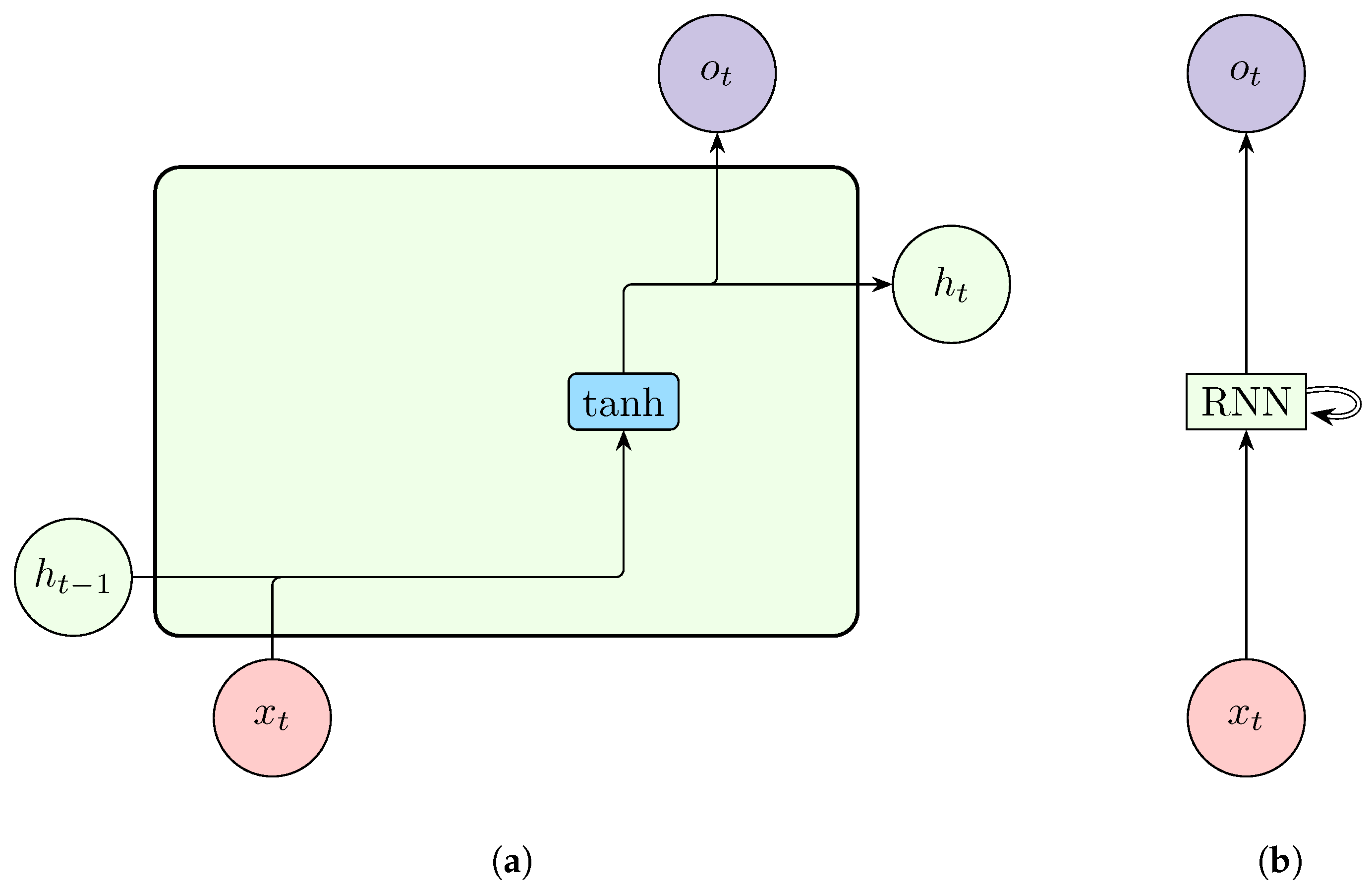
Simple RNNs use RNN cells which are stacked together to create an RNN. An RNN cell accepts two inputs at each time step; the previous hidden state, which encodes previous information, and the input at the current time step.
Figure 4.
A representation of a simple Recurrent Neural Network cell (a) and a single-layered unrolled Recurrent Neural Network (b).
Figure 4.
A representation of a simple Recurrent Neural Network cell (a) and a single-layered unrolled Recurrent Neural Network (b).
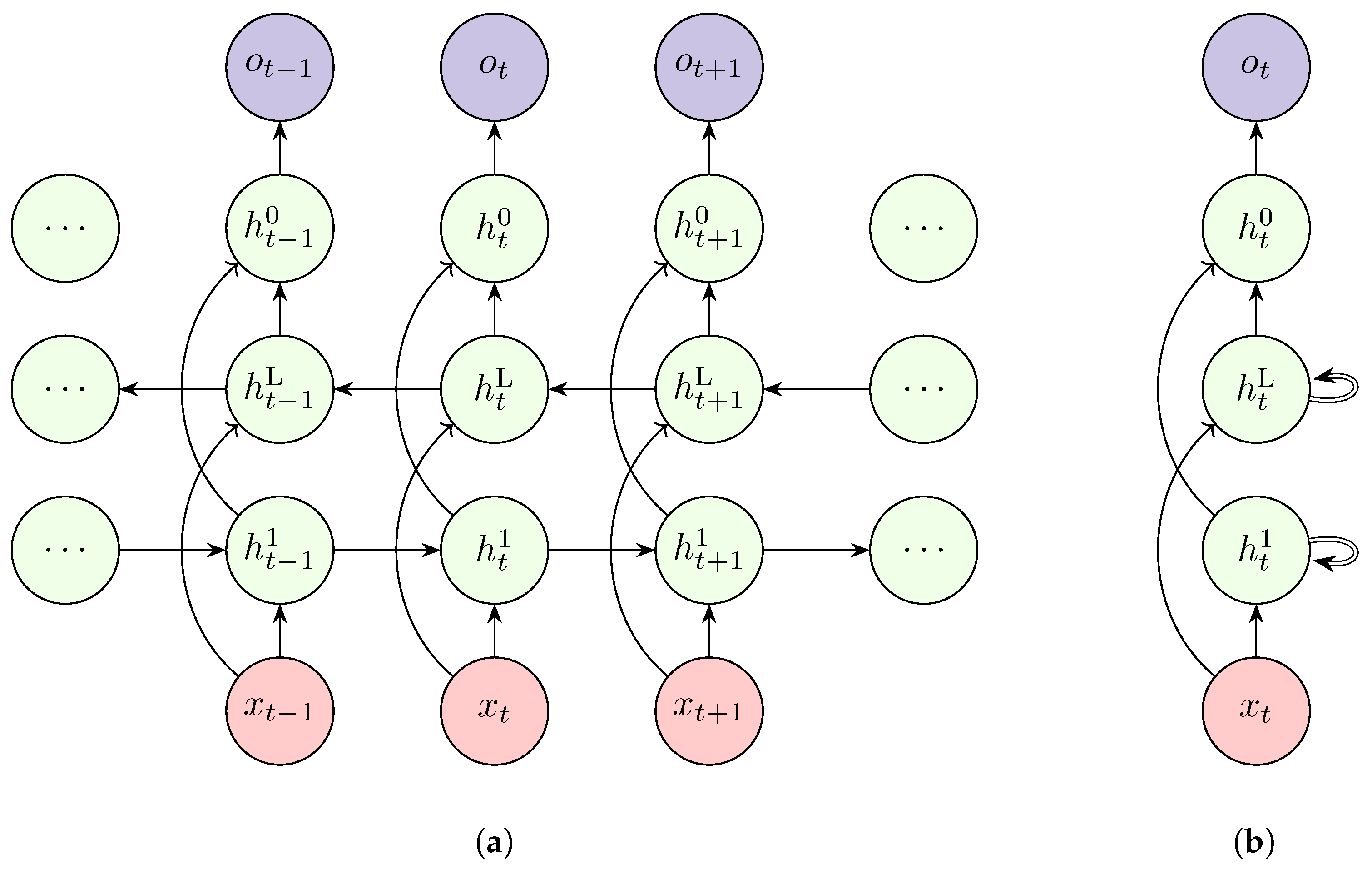
4.2.2. Deep RNN
The typical RNN discussed so far only considers a single layer. However, as indicated earlier, neural networks perform better with depth. Just as MLPs, this is possible with RNNs. Multiple RNN layers are stacked on top of each other as shown in Figure 5 to compose a Deep RNN. Cells in the top layers get input from the previous cell of the same layer as well as from the bottom layer.
4.2.3. Bidirectional RNN
To help address issues like missing values, RNNs use an innovative architecture called bidirectional recurrent neural network(BiRNN). This architecture was proposed by Schuster and Paliwal [111]. BiRNN combines two RNNs oriented in different directions with each RNN treated separately, i.e., for the forward RNN and for the backward RNN. The outputs of these networks are concatenated, i.e., , to produce the final output.
Figure 6.
Architecture of a Bidirectional Recurrent Neural Network (rolled(a) and unrolled(b)). Adapted from Vuong [110].
Figure 6.
Architecture of a Bidirectional Recurrent Neural Network (rolled(a) and unrolled(b)). Adapted from Vuong [110].
4.3. Comparisons of Standards RNNs
The three architectures of RNNs discussed thus far have some similarities and differencies. Simple RNNs offer a lightweight structure capable of modeling short-term dependencies; however, their effectiveness diminishes on long sequences due to vanishing gradients [112] and limited memory capacity . On the other hand, deep RNNs are able to learn hierarchical temporal features and tend to perform better than simple RNNs. Despite improving model accuracy, the added depth adds a layer of complexity and there is always a tradeoff between accuracy and model generalization. Thus, careful regularization and initialization are needed in deep RNNs to mitigate training instability. BiRNN’s introduce a layer of complexity with their dual encoding feature. This architecture is useful in applications such as anomaly detection, classification or data imputation tasks where the entire sequence is available a priori . However, bidirectionality is inherently noncausal and thus unsuitable for real-time forecasting, where future observations are not accessible. Despite these differences, all RNNs share a common advantage, weight sharing. Weight sharing reduces the number of trainable parameters in RNNs and thus reducing the computational costs

Table 2.
Comparison of Simple RNN, DRNN, and BiRNN in Time Series Modeling.
| Aspect | Simple RNN | Deep RNN | Bidirectional RNN |
|---|---|---|---|
| Temporal direction | Forward only | Forward only | Both |
| Long-term memory | Poor | Improved | Strong (non-causal) |
| Depth and abstraction | Shallow | Hierarchical | Context-rich |
| Suitability for forecasting | Online / short horizon | Long horizon forecasting | Not suitable for real-time use |
| Computation and training | Efficient, stable | Expensive, harder to train | High overhead |
| Best use case | Basic time series tasks | Multiscale or nonlinear time series | Offline classification or anomaly detection |
4.4. Shortfalls of RNNs
There are two main problems with the discussed RNN architectures. Firstly, RNNs are trained through a process called backpropagation through time (BPTT), which involves going back in time n steps to compute the derivative of the loss. Thus, the gradient of the loss function involves repeated multiplication of the Jacobian matrix of the hidden state transition,
If the largest eigenvalue of this matrix is less than 1, gradients tend to vanish. On the other hand, if is greater than 1, gradients grow exponentially, leading to the exploding gradient problem (unstable training) [15,113].
There are different ways to resolve these issues including gradient clipping, proper weight initialization, and use of gating mechanisms (LSTMs and GRUs). This issue is also tackled via training technique called teacher forcing, where ground truth at t is fed as input to the cell at [70].
A second shortfall of RNNs, which is also common to their advanced variants, is their lack of parallelizability, as they process data sequentially. This can significantly slow down training times. Attempts to resolve this have led to the development of advanced architectures such as transformers and parallelizable RNNs.
4.5. Long Short-Term Memory
To handle long and short sequences effectively without issues such as exploding or vanishing gradients, Long Short-Term Memory(LSTM) networks were introduced [65]. LSTM neural networks use a cleverly designed cell (LSTM cell) instead of the simple RNN cell. These gates are depicted in Figure (Figure 7).
The input to the forget gate is the previous hidden state and current input
acts as a mask for the cell memory since a sigmoid function squashes all outputs into values between 0 and 1. Zero entries erase irrelevant previous memory contents at a specific memory location.
To update the cell memory, an LSTM uses the following equations,
The input gate controls how much new information, which is represented by the candidate memory , should be stored in the cell state . It decides what proportion of the candidate memory will be added to the current memory, effectively controlling the flow of information into the cell state. The candidate memory represents a potential new memory value that could be added to the cell state. Its value is computed based on the current input and previous hidden state, capturing the new information to be incorporated into the cell state. The input gate modulates this candidate memory and determines how much of it should influence the memory update.
The current hidden state is then calculated based on the updated memory. A copy of the current memory is passed through a tanh activation function to normalize it between -1 and 1. This result is then multiplied by , which is computed as
The current hidden state, given by
along with the current cell memory , are passed to the next LSTM cell.
4.6. Other LSTM Variants
Different variations of the LSTM cell exist. The focus here is on the peephole LSTM [115] and xLSTM [116] The peephole LSTM extends the standard LSTM architecture by adding connections from the internal cell state to the input, forget, and output gates. The main benefit of this approach is improved gradient flow, which aids in mitigating the vanishing gradient problem. In contrast, xLSTM approaches a similar problem by incorporating additional gates for finer control over information retentions. The architecture also includes an exponential gating mechanism in which exponential activation functions are used in the input and forget gates to better manage data flow
4.7. Gated Recurrent Unit
The Gated Recurrent Unit(GRU) [117] was designed to simplify the LSTM while maintaining comparable accuracy. The GRU removes the need for a separate memory cell and reduces the number of gates to two; the reset gate and the update gate .
Figure 8.
Internal structure of a Gated Recurrent Unit(GRU) [114].
Figure 8.
Internal structure of a Gated Recurrent Unit(GRU) [114].
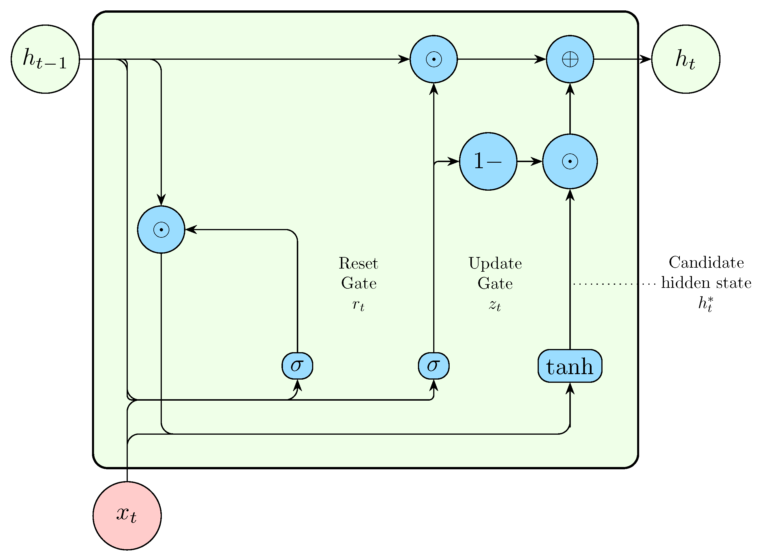
The reset gate controls how much of the previous hidden state should be considered irrelevant for the current time step. The input to the reset gate is the current input and the previous hidden state
After applying the logistic sigmoid activation, determines how much of the previous hidden state should be reset. Next, the candidate current hidden state is calculated by multiplying the reset gate output with the previous hidden state , and then adding the current input
The update gate determines the balance between the previous hidden state and the candidate current hidden state. A value of 0 completely ignores the previous hidden state and only considers the current input. Conversely, a value of 1 completely ignores the current input and only considers the previous hidden state. The update gate is computed as
Finally, the current hidden state is calculated as a linear interpolation between the previous hidden state and the candidate hidden state based on the value of ,
4.8. Comparison between LSTM and GRU
Both the LSTM and GRU were designed to solve the issue of vanishing gradients and enable long term modeling. The subtle difference between the two architectures is mostly in the cell complexity, where the number of gates in the GRU is reduced to two. While both models perform well on many sequence modeling tasks, GRUs often generalize comparably to LSTMs with less computational cost, making them a preferred choice in scenarios with limited resources or smaller datasets. However, in tasks that require modeling more intricate temporal dynamics, LSTMs may offer better performance due to their more expressive gating mechanisms. For more expressive modeling, in practice, it is also common to use deep or bidirectional RNNs with the LSTM or the GRU as the central computing mechanism.
4.9. Transformer Models
Transformers [118] were introduced to address the limitations of recurrent neural networks (RNNs). The issues referred to here are long-term memory and parallelization. Tranformers rely on self-attention to capture contextual dependencies across input sequences. Mathematically, self-attention is defined as
where , , and represent the query, key, and value matrices, respectively, and d denotes the dimensionality of the key vectors. To ensure causality, which is a key issue in time series, masking is used to prevent information from future time steps from influencing the current prediction.
Original transformer models were designed for machine translation tasks. However, over the past few years, transformers have been adapted to time series analysis due to their ability to capture long-range dependencies and enable parallel computation. Notable variants include Temporal Fusion Transformer (TFT) [119], Informer [120], Autoformer [121], FEDformer [122], and PatchTST [123].
4.10. Mamba
Mamba [124] is a recent architecture for efficient and expressive sequence modeling. This architecture was developed to overcome the quadratic complexity of self-attention in Transformers. It builds on discrete-time state space models (SSMs), represented by
Unlike classical SSMs, Mamba introduces input-dependent parameters , , and a dynamic step size , enabling selective compression of relevant information and improved adaptability. To extend memory and enable parallelization, Mamba uses structured initialization, (HIgh-order Polynomial Projection Operator) [125] for and a hardware-aware parallel scan algorithm.
4.11. Convolutional Neural Networks
Convolutional neural networks (CNNs) are among the most popular architectures and have significantly influenced the modern era of deep learning. CNNs were initially developed to handle grid-like data such as images. However, researchers have found CNNs to perform well on sequential data, such as time series. It has to be noted that time series can be considered one-dimensional grid data [109]. The fundamental operation in a CNN is the convolution. Mathematically, for the one dimensional discrete case, this is defined as,
where G is the input signal, H is the filter or kernel, * denotes convolution operator, i is the output index, m is the summation index, is the value of G at m, and is the flipped and shifted version of H.
Convolutions can also be multidimensional. For 2D convolutions, the operation becomes,
As can be seen, a typical convolution operation involves flipping the function H (kernel).However, in CNNs, it is uncommon to flip function H before applying it, so the operation is more accurately described as cross correlation[126].Despite this, the term convolution is still commonly used. The purpose of CNNs is to learn a set of functions H, also known as filters or kernels. These filters are typically small tensors (e.g., 1x1, 3x3, 5x5, or 7x7). For multi-dimensional inputs, the filters are extended accordingly. Unlike MLPs, CNNs rely on local connections and share the same filter across the entire input to create the output feature map. Multiple filters can be used in one layer, and their outputs are concatenated to form a complete feature representation. The dimensions of the feature map are dependent on the number of kernels, padding, stride, dilation, pooling, and upsampling. Since the same filter is reused across the input, CNNs are able to learn spatial relationships invariant to transformations. Additionally, CNNs require fewer parameters compared to fully connected networks, making them well-suited for high-dimensional data. Unlike RNNs, CNNs are parallelizable.
4.11.1. 1D CNN
The most basic CNNs used for time series are 1D CNNs [127]. This involves sliding the filter along the sequence length from the beginning. Notably, 1D CNNs can be used for multivariate time series modeling as well, provided that the filter width matches the width of the sequence. Despite their effectiveness, 1D CNNs suffer from future data leakage, violating causality.
4.11.2. Causal CNN
To overcome the issue of future data leakage in 1D CNNs, causal convolutions are used. Mathematically, causal convolution is written as,
Causal convolutions only use past data to make predictions. To handle long sequences, dilated convolutions, introduced by Yu and Koltun [128] are used to increase the receptive field with fewer layers,
This generalization allows flexible dilation without modifying the filter. The standard convolution is a special case where .
4.12. Graph Neural Networks
In several practical applications, time series emerge within networked structures such as road networks, water distribution systems, and railway infrastructures. In such settings, the data exhibit dependencies that are both spatial and temporal in nature. To capture these dependencies accurately requires their explicit modeling. Graph Neural Networks(GNNs) are a natural architecture for this as they provide a more flexible way to model such dependencies. Graph Neural Networks that take into account the aspect of time are called dynamic. In this section, we will firstly discuss the fundamentals of GNNs and will then consider how they fit in time series analysis.
Typically, the input to a GNN is a graph, e.g. a protein structure, social network, transportation network, etc. A graph is defined by a set of nodes , a set of edges , and associated mappings that describe the relationships between nodes. Mathematically, a graph is represented either through an adjacency list or adjacency matrix (A). The latter is widely used in Graph Neural Network applications. Each element in A indicates the existence or absence of an edge between a pair of nodes, i.e., if there is an edge from node i to node j, and otherwise. The specific structure of A depends on the type of graph. Graphs can have single or multiple edges between a pair of nodes. It is also possible to have edges which start and terminate on the same node (self-loops). Further categorisation of a graph depends on edge- directionality and edge-weight. Thus, graphs can be classified as directed or undirected as well as weighted or unweighted. A special case which will be our focus are undirected graphs without self-loops or multiple edges. The analysis of such graphs is simple since the adjacency matrix is symmetric.
Node ordering in a graph is arbitrary as such different formulations of the adjacency matrix are possible [84]. For this reason, a permutation matrix P is used to ensure that the output of the GNN remains invariant to the ordering of nodes. This is achieved through permutation-invariant embeddings and a transformed adjacency matrix .
In general, the goals of a GNN span a variety of tasks, including node classification [129], link prediction [130], graph classification [131], and graph generation [132] . A GNN aims to map the input node or edge features into an embedding space that offers a rich representation for further modeling [133]. These node or edge features are continuously updated by aggregating information from neighbouring nodes or edges through a process known as message passing,
where is a non-linear activation function, is the learnable weight matrix at layer t, AGG is a neighborhood aggregation function such as mean or sum, and denotes the set of neighbors of node v.
Message passing in a Graph Neural Network (GNN) occurs iteratively over several iterations. After a specified number of iterations t, each node encodes information about all other nodes in the graph. The number of iterations is considered optimal to ensure that the GNN has a sufficiently large receptive field while preventing oversmoothing; a scenario where all embeddings become indistinguishable [134]. The basic approach assumes all nodes and edges are of equal importance; however, more advanced methods have been developed to account for varying levels of importance.
4.12.1. Temporal Modeling in GNN
To make predictions, a GNN typically utilizes the final embedding layer. For temporal modeling, it is possible to integrate a GNN with other network architectures, where the final embedding layer is passed as input to subsequent neural network blocks. This approach is commonly used in temporal GNNs [135], where the final embedding is fed into another network block, such as an RNN or CNN. This allows the network to capture both spatial patterns using the GNN and temporal features using the RNN or CNN.
GNNs can also be used for data which is not spatial by nature. This is possible by first transforming the data into a graph structure. The approach seems to work quite well with time series. Liang et al. [136] employed this technique to impute missing values in traffic datasets. For a comprehensive overview of GNN applications in time series tasks, refer to Jin et al. [137].
4.13. Physics-Informed Neural Networks
Traditionally, the approach to training neural networks has been heavily data-centric. However, this approach may have drawbacks, such as noisy data that deviates from actual physical reality.To resolve this, researchers have been experimenting with the idea of incorporating the physics of a problem into a model. Enforcing physics into a model is a well studied field of machine learning under the umbrella of Scientific Machine Learning (SciML). Several studies have so far shown that models in scientific settings perform better on unseen data when the physics of the phenomenon being studied is considered [138] . Although SciML has been achieved through different techniques, our consideration in this review are Physics Informed Neural Networks (PINNs) [139] . PINNs are a household name in SciML hence their discussion. PINNs enforce physics through a physics regularization term which is added to the loss function. This is achieved through the problem’s differential equation and its associated conditions.
Consider the general form of a partial differential equation,
where represents a differential operator, is the solution to the PDE, and denotes the forcing term. The solution to this PDE must satisfy both initial and boundary conditions. Specifically, the initial condition is,
where is the initial time, and describes the initial state of the system. The boundary condition is expressed as,
where prescribes the behavior of the solution on the boundary of the spatial domain . Here, the spatial variable x spans the domain , and the temporal variable t lies within the interval .
The first step in a PINN is to calculate the residual of the PDE as follows,
Residuals are also calculated for initial and boundary conditions, and the total residual is termed the physics loss. Minimizing this loss across the domain and over the specified time interval is crucial for validating the accuracy and consistency of the solution under the given initial and boundary conditions. This ensures that the proposed solution adheres to both the dynamics described by the PDE and the constraints imposed by the initial and boundary conditions. However, in practice, exact satisfaction is rarely achievable; hence, PINNs do not perfectly satisfy the governing physics [140,141].
PINNs are usually trained by minimizing the following composite loss function,with each term adequately weighted,
where,
is the Initial Condition Weight, is the Boundary Condition Weight, is the Physics Weight, and is the Data Weight, all balancing their respective influences in the PIN model.
PINNs have been successfully applied to time series problems, such as the estimation of cuffless blood pressure [142]. A recent application of PINNs by Park et al. [143] involved weather data forecasting, where an RNN served as the backbone network and the harmonic oscillator equation was used to enforce physical constraints (see Figure 9).
Due to the nature of the harmonic motion solutions, the neural PDE component effectively modeled the seasonal component of the time series. This approach bears some similarity to the Fourier Analysis Network described earlier.
4.13.1. Issues with PINNs
Similar to other neural architectures, PINNs have shortfalls. A major shortfall lies in the training instability and difficulty in balancing the contributions of data loss and physics loss, especially when dealing with stiff PDEs or multi-scale phenomena [144]. This imbalance often leads to poor convergence or solutions that satisfy the data but violate the governing equations, or vice versa. Moreover, PINNs typically rely on automatic differentiation to compute residuals, which can be computationally intensive . Another notable challenge is the difficulty PINNs face in enforcing complex boundary conditions, especially in domains with discontinuities or sharp gradients [145]. A detailed investigation into the failure modes of PINNs and strategies to address them is provided by Krishnapriyan et al. [140].
5. Generative Modeling
In practical applications, there are scenarios where it is essential to model the input data itself. In such cases, a different class of models, generative models, may be more appropriate. Generative models learn the joint probability distribution and can use this distribution to generate new data points that resemble the training data. The aim of this section is to introduce various classes of generative models that are commonly employed for tasks such as data imputation and synthetic data generation in time series applications.
5.1. Autoencoders
The goal of an autoencoder is to learn a low-dimensional latent space of the data, and then to reconstruct the original data from this compressed space. An authoencoder achieves this using a decoder , for compression and , for reconstruction. Learning is done by minimization of the reconstruction loss, which is given by
Exact reconstruction is not possible because the latent space has a lower dimension than the input and output. However, this architectural design is necessary to encourage the autoencoder to learn useful features required for reconstruction.Different researchers have successfuly applied autoencoders to data denoising [146], data imputation [147], anomaly detection [148], and more. Despite its wide usage in literature, the standard autoencoder cannot perform meaningful data interpolation, and this arises from the discrete nature of the learned latent space [149]. Among other approaches, this limitation is addressed by variational autoencoders.
5.2. Variational Autoencoders
Unlike traditional autoencoders, variational autoencoders (VAEs) [150] adopt a probabilistic framework to learn a more structured latent space.
Figure 10.
Architecture of a Variational Autoencoder (VAE). The input x is passed through an encoder network to predict the variational parameters: and , which parameterize a Gaussian variational distribution . A latent variable is sampled from this distribution using the reparameterization trick: , where . This sample is then fed into the decoder , to predict the data x. Adapted from Prince [84].
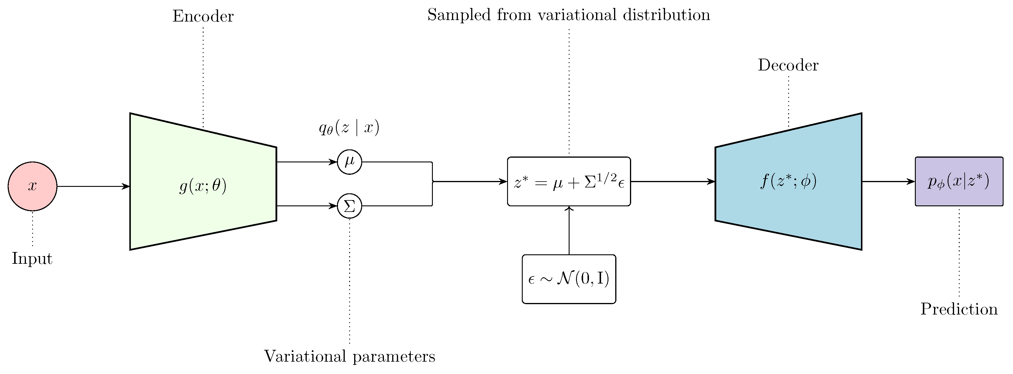
First, the input is mapped to a latent space z using an encoder , where . Since is generally intractable due to the intractability of the marginal likelihood , VAEs introduce a more tractable approximate posterior . Then, to reconstruct the data from the latent space, a decoder is used.
VAEs are trained by maximizing the marginal likelihood over the reconstructed sample, , which is obtained by marginalizing over the latent space,
This integral is generally intractable and is typically simplified to provide tractable proxy objectives. By introducing a variational distribution , we can apply Jensen’s inequality to get lower bound of the log marginal likelihood,
This gives rise to the evidence lower bound (ELBO),
Intuitively, the first part of this expression represents the reconstruction term, which encourages the decoder to accurately reconstruct the input data. The second term encourages the variational distribution to be as close as possible to the prior. It is common not to sample directly from , but rather to use a reparameterization trick (Equation 41),
This allows the expectation over to be rewritten as an expectation over a fixed noise distribution . Expression (40) can therefore be rewritten as a reparameterized objective
According to Gundersen [151], without the reparameterization trick, backproping would not compute an estimate of the derivative of the ELBO and would thus give no guarantee that sampling large numbers of z will help converge to the right estimate of the gradient. The gradient of the ELBO is computed with respect and via
5.3. Generative Adversarial Network
A Generative Adversarial Network (GAN) [126] aims at generating realistic data similar to real-world data present during training by fooling another network into believing that the generated samples are real. This is achieved by simultaneously training two networks: a generator G and a discriminator D.
Figure 11.
Schematic of a Generative Adversarial Network (GAN) training loop. A latent variable z is sampled and transformed by the generator to produce samples. These, along with real data , are evaluated by the discriminator , which outputs the probability of each sample being real. The discriminator is updated to better distinguish real from generated, while the generator updates its parameters to fool the discriminator.Adapted from Calin [155].
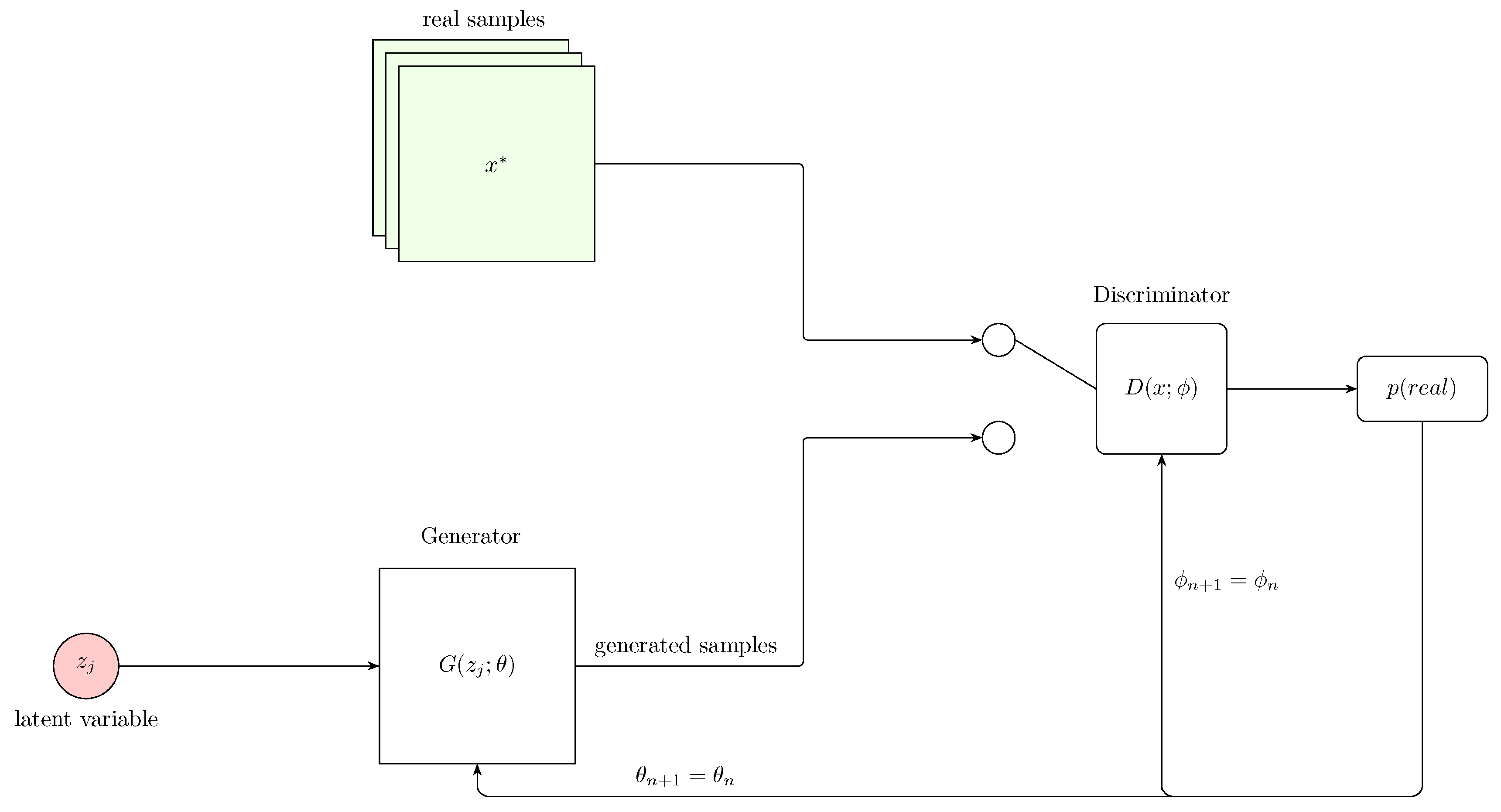
The generator creates samples from a latent variable . The objective of the generator is to produce data that is indistinguishable from real data. Mathematically, this is equivalent to minimizing the following expression with respect to ,
Technically, if samples are assigned a higher probability, i.e., if the discriminator classifies them as being real, the above expression approaches zero. However, if generated data is classified correctly, i.e., a low probability is assigned to generated data, the expression tends to infinity. This means that the generator loss can only be reduced if the discriminator incorrectly classifies generated data, in which case the generator achieves a minimum loss.
As already highlighted, the discriminator is responsible for classifying data as being real or generated(binary classifier). The input to the discriminator is either a generated or real sample, and it returns a probability that is higher when a sample is real (i.e., close to 1). The objective of the discriminator is usually to maximize the following expression with respect to
Despite the fact that the underlying principle behind GANs is conceptually straightforward, they are difficult to train in practice. A major challenge is mode collapse, where the generator ignores the variability in the latent space and produces limited or nearly identical output [84,156]. To address this issue, several techniques have been proposed. They include feature matching and mini-batch discrimination [157], unrolled GANs [158], Wasserstein GANs (WGAN) [159], spectral normalization [160], and gradient penalty methods (e.g., WGAN-GP) [161].
Although GANs were initially developed for image data, they have since been extended to handle sequential data such as time series data. Notable adaptations in this space include TimeGAN [162], SeriesGAN [163]; FinGAN [164] to name a few. For a detailed survey of GAN applications in time series, the works of Brophy et al. [165] and Zhang et al. [166] can be consulted.
5.4. Normalizing Flows
Instead of implicitly modeling the data distribution like GANs, normalizing flows explicitly model the probability distribution over the data [84]. Normalizing flows transform a simple distribution over a latent variable into a more complex distribution using differentiable and bijective transformations (see Figure 12).
The transformation function is usually parameterized by a neural network. Transformations are required to be differentiable and bijective so as to ensure a smooth transition between the latent and data space while enabling efficient learning via gradient-based methods. Several techniques have been developed to design transformations with these desired properties. Among them are coupling flows [168,169], neural ODEs [170], and autoregressive flows [171].
Since the data distribution is defined through a transformation, its density is determined using the change of variables formula,
where .
The objective is then to maximize the likelihood of the data under this model, i.e.,
Recent studies have applied normalizing flows to capture complex temporal dependencies and uncertainty in time series. Rasul et al. [172] proposed a graph-augmented normalizing flow (GANF) using Bayesian networks to model inter-series causality.Flow based modeling has also been combined with temporal and attribute-wise attention for high-dimensional, label-scarce data [173]. In forecasting, Rasul et al. [172] integrated autoregressive models with conditional flows to enhance extrapolation and capture temporal correlations. Fan et al. [174] proposed a decoupled formulation called instance normalization flow (IN-Flow), which addresses distribution shifts via an invertible transformation network.
5.5. Diffusion Models
Diffusion models (DM) [175] are trained by sequentially adding noise to a data sample over multiple time steps and then attempting to remove this noise. The noise is added according to a Markovian process
with its associated distribution,
is a hyperparameter which determines how quickly the noise gets blended. This hyperparameter can be fixed across all time steps or it can vary according to a predefined schedule. While single-step updates are possible for adjacent time steps by applying Equation 48, it is usually helpful to be able to move directly from to in a single step as well. This is important especially in the reverse process when denoising. The expression required to do this can be derived by generalizing Equation 48 over multiple time steps and is expressed as,
Derivation of this expression takes advantage of the properties of sums of Gaussian random variables. On the other hand, during the reverse process, the transition process is modelled as,
with an associated transition probability . Here, is a standard normal distribution used for reparameterization. is the noise predicted by the neural network, which is parameterized by . The goal is to learn a mapping that makes and as close as possible, which leads to the following loss function,
In other words, the model tries to predict the amount of noise that was added to the data sample during the forward (diffusion) process.
The discussion thus far has primarily focused on denoising diffusion probabilistic models (DDPMs), often considering the unconditional generation setting where the data distribution is modeled without auxiliary information. However, general DMs are also capable of conditional generation, where the data distribution is modeled given some conditioning variable such as class labels or other contextual attributes. DMs have been proposed for forecasting [176,177,178], classification [179,180], anomaly detection [181,182] , imputation [183,184], and generation Narasimhan et al. [185], Chi et al. [186]. A comprehensive review of the use of diffusion models in time series has been conducted by Lin et al. [187], covering key models, methodologies, and applications across forecasting, imputation, and generation tasks. More recently, Yang et al. [188] have provided an extensive survey encompassing both time series and spatio-temporal applications of diffusion models, categorizing existing approaches based on task type and model structure.
5.6. Autoregressive Models
Given a sequence, , the joint probability distribution can be factorized using the chain rule of probability,
where .
This is called an Autoregressive model (ARM) and it allows for the exact computation of the likelihood [189]. To capture complex dependencies within the data, each conditional distribution in equation Murphy [190]is parameterized by a neural network. Tomczak [191] provides good cases for ARMS. Generally, the conditional distribution can be modelled as it is, but in practice, it usually computationally expensive as the sequence length .An alternative approach employs the first-order Markov assumption to simplify the conditional distribution at time t.Thus, the conditional distribution at time setstep t depends only on the immediate previous time step , i.e.
An ARM is trained by maximizing the likelihood of the observed data. This is also equivalent to minimizing the negative log-likelihood (NLL) given by
Once trained, data generation follows an ancestral sampling procedure, where values are sequentially sampled based on the learned conditionals.
5.7. Energy-Based Models
Energy-Based Models (EBMs) offer a general framework for modeling probability densities by associating scalar energy values to configurations of the input space.EBMs have their origins in statistical physics.The underlying assumption is that observed, high-probability data should correspond to low-energy states, while implausible or unlikely configurations should be mapped to regions of higher energy.
Formally, the model defines an unnormalized density over via a Boltzmann distribution,
Here, is a learned energy function, typically parameterized by a deep neural network, and is the partition function that ensures the density integrates to one. However, this normalization term is generally intractable in high dimensions, rendering exact likelihood evaluation and sampling computationally prohibitive. The parameters of the energy function are found through maximum likelihood estimation, which results in the following objective function,
with the gradient given by,
The first term is readily computable using observed data, while the second requires samples from the model distribution, which is itself defined implicitly by the energy function. Consequently, much of the complexity in training EBMs arises from the need to draw samples from a model whose normalization is unknown. Markov Chain Monte Carlo (MCMC) methods, such as Langevin dynamics, are commonly used for this purpose [189].
Popular examples of EBMs in literature include Boltzmann Machines [192] and Hopfield Networks [62]. Similar to the other generative models, EBMs have also been applied to time series analysis. Brakel et al. [193] outlined the training strategy for training EBMs for data imputation.Yan et al. [194] proposed ScoreGrad, which a is multivariate probabilistic time series forecasting framework based on continuous energy-based generative models and has been found to achieve state of the art results on a number of datasets.
5.8. Summary of Generative Models
Table 3 presents a comparative summary of the generative models discussed.
6. Uncertainty Quantification
SHM data can be limited or noisy. Noise can emanate from different sources such measurement errors and environmental variability. Limited data might be due to sensor malfunction, missing data, and intermittent data collection due to huge costs associated with the process. Considering these factors, uncertainty quantification is critical to SHM for effective decision making. Uncertainties are generally classified as aleatoric and epistemic [83,195]. Aleatoric uncertainty is associated with inherent randomness and cannot be reduced. According to Wikipedia, epistemic uncertainty is associated with things which one could in principle know but does not know [196]. Thus, once knowledge is available, epistemic uncertainty can be reduced. Epistemic uncertainty is further grouped into two major categories: homoscedastic, meaning it is constant across all observations, or heteroscedastic, meaning it varies with covariates. While homoscedastic uncertainty is relatively straightforward to handle, heteroscedasticity introduces additional complexity into modeling tasks. If these uncertainties are not properly accounted for, model predictions are usually unreliable can may potentially lead to suboptimal decision-making.The goal of this section is therefore to discuss how uncertainties are handled in deep learning. We do this from a Bayesian context.
6.1. Bayesian Inference
In many practical scenarios, prior knowledge plays a critical role in shaping our understanding of a problem. However, conventional deterministic modeling approaches typically disregard this prior information. A significant limitation of such methods is their reliance on large volumes of data to achieve good performance. In reality, data is often limited, incomplete, or corrupted by noise. In the late 1980s and early 1990s, Denker et al. [197], Tishby et al. [198], Denker and LeCun [199], Buntine and Weigend [200], MacKay [201], Neal [202] and Neal [203] proposed the bayesian framework as an alternative learning method. This approach provides a way to incorporate prior knowledge into a model as well estimate uncertainties associated with its outputs. The central idea that governs this philosophy is Bayes’ rule. Mathematically, Bayes’ rule is expressed as
where is the posterior, is the likelihood, is the prior, and the evidence term is given by,
To make predictions for a new data point in a supervised mode, the posterior predictive distribution is used,
With regards to this expression, Murphy [204] writes, "the posterior is our internal belief state about the world and the way to test if our beliefs are justified is to use them to predict objectively observable quantities."
Despite the simplicity of Bayes’ rule, the posterior distribution is often analytically intractable in real-world applications. For deep neural neural networks, the parameter vector may contain millions or even billions of parameters. For this reason, Bayesian methods were historically not favored for training deep models. However, this has changed with the development of efficient approximation techniques. Common methods for parameter estimation are discussed in the following sections.
6.1.1. Analytical Methods (Conjugacy)
For certain combinations of the prior and likelihood, the posterior can be computed analytically. In this case, the posterior distribution is of the same functional form as the prior, and the likelihood-prior pair is known as a conjugate pair [83].Besides providing a closed form solution for the posterior distribution, conjugacy enables sequential learning where the posterior at t becomes the prior at . Some of the conjugate pairs include Gaussian-Gamma, Gaussian-Inverse-Chi-Squared, Gaussian-Inverse-Gamma, and Gaussian-Inverse-Wishart [205].
6.1.2. Maximum Likelihood Estimation
Although not Bayesian, Maximum Likelihood Estimation (MLE) is widely used to estimate model parameters. The goal of MLE is to find the set of parameters that maximizes the likelihood of the data,
Equation 61 considers that the data is identically and independently distributed (i.i.d.). For large datasets, the computation of the likelihood can result in numerical instability. Large values of of result in overflow, while small values result in underflow. It is important to note that is a likelihood function, not a probability, and therefore can take values greater than 1.
To improve numerical stability and make the expression amenable to optimization, the log-likelihood is considered instead. Applying the properties of logarithms, the log-likelihood function is given by,
The above equation is a non-convex function and would otherwise benefit from readily available convex optimization algorithms by considering the negative log likelihood. This, in theory, is possible by taking the negative of the function. Thus, it is common to encounter negative log-likelihood in optimization problems
Maximization of the log-likelihood is similar to the minimization of the negative log-likelihood, and thus to find the optimal parameters,
A key limitation of MLE is its tendency to overfit, which can be mitigated using priors, leading us to Maximum A Posteriori estimation.
6.1.3. Maximum A Posteriori (MAP)
Bayes’ rule can be rewritten, omitting the marginal likelihood (which is constant w.r.t. ) as,
With this expression , it is possible to maximize the unnormalized posterior directly, i.e.,
Taking the log for numerical stability,
The second term serves as a regularization term, and this form is structurally similar to penalized optimization.
6.1.4. Laplace Approximation
The Laplace approximation is a technique used to approximate a posterior distribution with a multivariate Gaussian centered at the maximum a posteriori (MAP) estimate or, in some cases, the maximum likelihood estimate (MLE). It provides a way to account for uncertainty in the maximum likelihood or maximum a posteriori parameter estmates. Given a model with parameters , and a log-posterior function , the Laplace approximation takes the following form,
where is the MAP estimate given by equation 67 and the covariance matrix is approximated by the inverse of the negative Hessian of the log-posterior evaluated at ,
This approach captures the local curvature of the posterior distribution around the mode, thereby providing a second-order approximation of the distribution [83]. However, computing the full Hessian matrix is often computationally expensive, especially in high-dimensional parameter spaces. As a result, various approximations and low-rank techniques have been proposed to reduce this burden.
6.1.5. Expectation Maximization
The procedures for MLE and MAP discussed so far assume that the dataset is complete and that all variables associated with the model are fully observed and known. However, in many practical applications, models often involve partial data or incorporate latent variables that are not directly observable. In such scenarios, the complete log-likelihood must account for these hidden variables, necessitating marginalization over them to obtain the observed data likelihood. Our derivation of the E-M algorithm is based on the work of Gao [206].
Formally, let represent the observed dataset, the corresponding latent variables, and the parameters of the model. The complete-data log-likelihood is given by
However, since the latent variables Z are unobserved, the quantity of interest becomes the marginal log-likelihood
where the integral is taken over all possible configurations of the latent variables. In models containing a large number of latent variables, this integral typically becomes intractable, either due to high dimensionality or the complexity of the joint distribution .
To address this intractability, an arbitrary probability density function over the latent variables is introduced. By doing so, the marginal log-likelihood can be rewritten as
This re-expression enables the application of Jensen’s inequality, exploiting the concavity of the logarithm function to derive a lower bound. Specifically, Jensen’s inequality yields
which leads to
Defining the functional,
where denotes the entropy of , the above inequality can be compactly written as,
serves as a surrogate objective function that can be maximized in place of the intractable marginal log-likelihood.
Expectation-Maximization (EM) algorithm is a classical procedure for maximizing the marginal likelihood by iteratively optimizing the lower bound . EM algorithm proceeds in two alternating steps, referred to as the Expectation step (E-step) and the Maximization step (M-step).
In the E-step, given the current estimate of the model parameters , the function is set to the posterior distribution of the latent variables conditioned on the observed data and the current parameters,
Under this choice, the lower bound becomes tight, satisfying
thus removing the looseness introduced by Jensen’s inequality. The E-step therefore consists of computing the expected complete log-likelihood,
Following the E-step, the M-step seeks to update the model parameters by maximizing this expected complete log-likelihood
6.1.6. Monte Carlo Integration
Bayesian inference often requires evaluating integrals like the marginal likelihood, , which is equivalent to an expectation, . This can be approximated by sampling,
Where is the number of samples.Monte Carlo integration is useful in high-dimensional spaces where analytical solutions are infeasible. The accuracy improves with more samples.
6.1.7. Importance Sampling
The typical monte carlo assumes that all samples are equally likely, which may not hold for heavily-tailed distributions such as the Gaussian. In such cases, a more effective technique is needed to assign higher weights to high-probability points and lower weights to low-probability points in order to provide accurate estimates of integrals. This can be achieved by modifying the marginal likelihood integral as follows,
with being a simple distribution from which samples can be drawn efficiently. This transformation allows for reweighting samples according to the ratio . The integral is now written as an expectation with respect to
We approximate this expectation using Monte Carlo sampling. Drawing for , the marginal likelihood is estimated as
6.1.8. Variational Inference
Variational Inference (VI) is a method for approximating complex probability distributions in cases where exact computation is intractable. The goal is to approximate a posterior distribution with a simpler variational distribution .Such a variational distribution is considered close to the posterior distribution. Closeness is usually achieved by minimization of the Kullback-Leibler (KL) divergence between the variational distribution and the true posterior,
Minimizing this divergence is equivalent to maximizing the Evidence Lower Bound (ELBO), given by,
The ELBO essentially transforms a bayesian inference problem into an optimization problem and can thus be optimized using gradient-based methods, allowing efficient approximation of the posterior by . While VI is typically faster than sampling-based methods, it is not guaranteed to converge to the true posterior.
6.1.9. Markov Chain Monte Carlo
Markov Chain Monte Carlo (MCMC) methods use a Markov chain to generate samples from an unknown posterior distribution. The chain satisfies the Markov property, where the next state depends only on the current state,
A large number of samples are generated using the chain, which is designed so that its stationary distribution is the target posterior. Perturbations are added iteratively (as in a random walk), and new states are accepted with a certain probability. The stationary distribution satisfies,
If the chain is ergodic, this stationary distribution is unique and reachable from any initial distribution.
Metropolis-Hastings Algorithm
The Metropolis-Hastings (MH) algorithm is an MCMC approach that generates samples from a proposal (or transition) distribution , with acceptance based on a probability criterion. The MH algorithm was first proposed in 1950, and used a symmetric proposal distribution in its initial form. By symmetric, we mean that the probability of moving to state i was equal to the probability of returning to the starting state. This symmetric form is expressed as
Hastings [207] improved upon the algorithm by incorporating asymmetric proposal distributions.
The MH algorithm uses the following criteria to move to new states: if the proposed sample is greater than the previous sample, the new sample is accepted. And if the proposed sample is less than the current sample, the new sample is accepted with an acceptance probability
This recursive process continues until the chain reaches a stationary distribution. One drawback of the MH algorithm is that random sampling can result in slow convergence and correlated samples. The subsequent method, Hamiltonian Monte Carlo (HMC), addresses this issue by incorporating gradient information to enhance sampling efficiency.
Hamiltonian Monte Carlo (HMC)
The Hamiltonian Monte Carlo (HMC) is a sampling-based parameter estimation approach that uses a systematic approach to sampling. To enable faster and efficient exploration of the target distribution, HMC leverages its gradient information. HMC employs Hamiltonian mechanics, incorporating both position q and momentum p. The core principle is to simulate the trajectory of a particle moving through a potential energy landscape defined by the target distribution.
In HMC, the potential energy is related to the target distribution . The kinetic energy and Hamiltonian are expressed as,
where M is the mass matrix. The Hamiltonian governs the dynamics of the system via Hamilton’s equations,
To approximate these dynamics, HMC uses the leapfrog integrator. The updates for momentum and position are,
Finally, the acceptance probability for the proposed state is calculated as,
More extensive treatments of HMC and its variations can be found in Marwala et al. [208]
6.2. Bayesian Neural Networks
6.2.1. Overview
Within a Bayesian context, model parameters are treated as distributions rather than point estimates [209]. The objective of a Bayesian Neural Network(BNN) is to learn these distributions. To this end, different methods have been developed to quantify uncertainty in neural networks. The discussions in this section will focus on 4 methods and the rationale for this choice is simplicity and similarity of each approach to the classic backpropagation. The first approach is discussed mainly because it has been extensively applied to SHM and can easily be scaled.
6.2.2. Tractable Approximate Gaussian Inference
The Tractable Approximate Gaussian Inference (TAGI) [210] is a probabilistic method that allows for the analytical inference of model parameters without relying on backpropagation. TAGI achieves this through a two-step process: propagation of the model uncertainty using moment functions and local linearization of the activation function. Parameters are then updated using a modified Rauch–Tung–Striebel (RTS) algorithm [210,211]. TAGI makes some assumptions about network parameters, layers, and units within layers. Parameters and units within a layer are considered i.i.d. and normally distributed. TAGI also uses the inherent conditional independence between hidden layers, i.e. .
Consider a neural network with an observation model described by
Mathematically, the i-th hidden state of the -th layer can be written as
where is the hidden state of the -th layer, is the weight from the k-th neuron in layer j to the i-th neuron in layer , is the activation of the k-th neuron in layer j, and is the bias term for the i-th neuron in layer .
To propagate uncertainty, TAGI uses the Gaussian Multiplicative Approximation (GMA) given by the following equations
While the sum of Gaussian variables remains Gaussian, the same is not generally true for their product. Equation 97 poses this challenge, as it involves the product of two random variables, i.e., and .
However, under the GMA and with a sufficiently large number of hidden units, the resulting distribution can be shown to converge to a Gaussian, .
Thus, TAGI is theoretically capable of approximating the moments of the hidden states. It is important to note that, although the propagation of information from the input layer to the output layer utilizes nonlinear activation functions, TAGI employs a locally linearized version of this transformation for the hidden state inputs. This linearization facilitates operations involving Gaussian random variables since a linear transformation of a Gaussian random variable results in another Gaussian random variable. TAGI achieves this by locally linearizing the nonlinear activation function about using a first-order Taylor approximation. It is crucial to emphasize that this local linearization does not imply the use of a linear activation function. Instead, for each input covariate , the linearization is performed at different , thereby preserving the nonlinear relationship between the inputs and the outputs .
Since TAGI assumes that the model parameters and hidden states are independent, it is computationally efficient, operating with a complexity of , where is the number of hidden units per layer, and scales linearly with hidden layers . So far, numerous enhancements have been made since the original implementation of TAGI. For instance, Deka et al. [212] extended TAGI to account for heteroscedastic uncertainty (Figure 13).
6.2.3. Learned Observation Noise in TAGI
Instead of treating as a fixed term, it is now learned from the data using the following equations,
where
and
Note:
6.2.4. Further TAGI Extensions
TAGI has also been successfully extended to address problems involving sequential data, particularly in time series modeling. Recently, Vuong et al. [213] developed the theory for modeling uncertainty in LSTMs and Gated Recurrent Units (GRUs) using TAGI as the foundational learning algorithm.
6.2.5. Monte Carlo Dropout
Dropout [214] is a method to mitigate overfitting in neural networks. During model training, dropout randomly freezing a subset of nodes (typically 50%) by setting their values to zero. The overall effect of this is that the network is less dependent on any individual weight. Once the model is trained, dropout is no longer applied.
Monte Carlo (MC) [215] dropout reinterprets dropout as a method for performing approximate Bayesian inference. A similar dropout procedure is applied during inference, and multiple forward passes are performed on the same input. This repeated stochastic sampling allows estimation of the predictive uncertainty by treating each forward pass as a sample from the posterior predictive distribution.
In principle, the final output of an MC dropout is considered an ensemble of outputs from different stochastic realizations of the network.
MC dropout is attractive due to its simplicity in implementation. However, it is computationally expensive during inference, as multiple forward passes must be performed. Additionally, the uncertainty estimates produced by MC dropout are often poorly calibrated.
6.2.6. Bayes by Backpropagation
As already highlighted, the goal of a BNN is to learn distributions of the network weights. The posterior distribution of these weights, , is generally intractable since neural networks contain a huge number of weights. This renders the marginal likelihood intractable as well. As already discussed, the standard variational approach employs a more tractable distribution to approximate ; with the Gaussian distribution being a common choice. As is always the case in VI, the goal is to make as close as possible to . This is achieved through minimization of the Kullback-Leibler divergence. We won’t discuss the full details of the derivation of the loss function used in Bayes by backprop as it can be easily derived using same principles used in Section 5.2 and Section 6.1.8. Bayes by backprop [216] uses a similar technique to VAE (reparamaterization trick) to express the gradient of an expectation as an expectation of the gradient. This allows us to compute gradients based on the reparameterization parameters and use standard backpropagation to update the network weights.
6.2.7. Probabilistic Backpropagation
Due to its reliance on sampling during both training and inference, the Bayes by backprop is not scalable. An alternative, scalable approach is the probabilistic backpropagation (PBP) [217], which was developed by researchers at Havard. PBP models each weight as a univariate Gaussian. These weights are learned via forward and backward passes through the network, just like in classic backpropagation. During the forward pass, input is propagated through the network. However, since the weights are random, activations at each layer are also random, though this time more complex and intractable. PBP approximates these intractable distributions with tractable Gaussians using moment matching. At the end of the forward pass, PBP uses the marginal probability of the target variable to measure performance and the gradient of this expression is computed with respect to the means and variances of the approximate distributions. The gradient is then propagated back to update the means and variances of the weights. Unlike classic backpropagation, PBP uses Assumed Density Filtering (ADF) for the parameter updates. ADF is a principled sequential way of minimizing the Kullback-Leibler divergence and is useful in PBP considering that we are building the posterior sequentially from more tractable distributions.
7. Applications
Deep learning for time series have been employed in various applications within SHM. We conducted a systematic literature search to identify studies on deep learning for time series analysis in SHM. The following search querry was used to retrieve articles from the scopus database:
(TITLE-ABS-KEY ("deep learning" OR "neural network" OR "variational autoencoder" OR "VAE" OR "recurrent neural network" OR "RNN" OR "long short-term memory" OR "LSTM" OR "gated recurrent unit" OR "GRU" OR "convolutional neural network" OR "CNN" OR "temporal convolutional network" OR "TCNN" OR "diffusion model" OR "normalizing flow" OR "physics-informed neural network" OR "PINN" OR "Bayesian neural network" OR "BNN" OR "multilayer perceptron" OR "MLP" OR "transformer") AND TITLE-ABS-KEY ("time series*" OR "temporal" OR "forecast*" OR "causal*") AND TITLE-ABS-KEY ("structural health monitoring" OR "SHM")) AND PUBYEAR > 2019 AND PUBYEAR < 2025 AND (LIMIT-TO(SRCTYPE, "j")) AND (LIMIT-TO(PUBSTAGE, "final")) AND (LIMIT-TO(SUBJAREA, "ENGI") OR LIMIT-TO(SUBJAREA, "MULT") OR LIMIT-TO(SUBJAREA, "ENVI") OR LIMIT-TO(SUBJAREA, "EART")) AND (LIMIT-TO(DOCTYPE, "ar")) AND (LIMIT-TO(LANGUAGE, "English"))
Figure 14 summarizes the entire process, from the initial database search, through exclusion of irrelevant studies, to the identification of articles included in the final review.
Based on the identified studies, the applications were categorized into five thematic areas: damage assessment, structural response prediction, structural load prediction, data reconstruction, and anomaly detection. Each of these areas is explored in greater detail in the following sections.
7.1. Damage Assessment
Damage assessment includes the detection, localization, and quantification of structural deterioration. A wide range of approaches have been proposed to address this challenge. A hierarchical CNN-GRU framework was developed to exploit both spatial and temporal information for structural damage detection in bridge datasets [218]. Recognizing the importance of feature extraction, another study proposed a channel-spatial-temporal attention network to refine sample-specific features across multiple dimensions [219]. Offshore jacket platforms have also been a subject of interest, where a CNN-BiLSTM-Attention model, optimized via particle swarm optimization, demonstrated more than 95% accuracy in damage detection [220].
In vibration-based damage diagnosis, several studies have focused on improving attention mechanisms and deep feature learning. A multi-head self-attention LSTM autoencoder was introduced for unsupervised diagnosis and quantification of damage in ambient vibration data [221]. The Transformer architecture was leveraged for post-disaster damage state classification using seismic data [222], and a custom 1DCNN-BiLSTM model with an Inception module was used to detect minor changes in RC beams [223].
Additional studies emphasized the localization of structural damage using various techniques. A time-varying damage index was proposed in conjunction with a 1D-CNN to enhance Lamb wave-based localization [224], while an autoencoder-based unsupervised model enabled accurate damage localization using raw acceleration data [225]. Localization has also been explored using acoustic emissions and arrival time distributions via LSTM and Bayesian methods [226], and through Transformer-based learning of multivariate vibration signals for submerged offshore wind turbine structures [227]. Damage classification using CNN and time-frequency analysis has been achieved through continuous wavelet transform representations of acceleration data [228], and Trident, a ConvLSTM3D model, achieved high-resolution damage identification in bridges [229]. Further work addressed unsupervised real-time detection using statistical modeling [230], sensor signal fusion via a 1D-CNN-LSTM hybrid [231], and the integration of Burg Autoregressive features with stacked autoencoders [232]. Multiclass damage detection and classification have also been explored. A 1D CNN method using windowed time series was validated for a full-scale bridge [233], while another study introduced a CNN model with synchrosqueezing transform to detect damage in the Z24 bridge [234]. Others investigated transformer-based models [235], metaheuristic optimization [236], and GAN-based signal augmentation [237]. Stochastic configuration networks [238] and hybrid CNN-RNN methods [239] have further enriched this task.
7.2. Structural Response Prediction
Predicting structural responses such as displacement, strain, stress, and vibration is fundamental in SHM. Deep time series have shown exceptional ability in capturing nonlinear temporal patterns, making them well-suited for this task. Seismic and environmental responses have been a primary focus. A Dung Beetle Optimization-enhanced BiLSTM model, integrated with discrete wavelet transforms, was used for seismic response prediction in slope reinforcement structures [240]. A dual-stage attention LSTM (DALSTM) encoder-decoder model was used for displacement forecasting in arch dams [241]. Another study used STL-extra-trees-LSTM modeling for a similar task [242].
Tunnel and bridge response prediction has also received extensive attention. LSTM-based approaches have been adopted for modeling stress and strain during shield tunneling [243], deflection predictions under vehicle and thermal loads [244,245] , and buffeting response forecasting in a bridge under aerodynamic effects [246]. An ensemble RNN with short-sequence LSTMs has been proposed for high-frequency health monitoring [247], while LSTM and CNN hybrid models have been introduced for rail track systems [248] and long-span bridge deck wind-induced lateral displacement responses [249]. Temperature-induced structural responses have been modeled in numerous studies. These include CNN-based prediction of long-term strain using weather data [250,251], a neural network based on hydrostatic-temperature-time (HTT) for predicting concrete dam displacement [252,253], and HTT enhancements via the DeepLift framework for dams in extreme climates [254]. BiLSTM models have also been used to map temperature fields to strain distributions [255]. Multi-factor response models have been implemented using attention-enhanced BiLSTM frameworks [256] and transformer-based architectures for long-term structural state forecasting and strain prediction [257,258]. Physics-informed models such as Phy-Seisformer [259] and simplified rheological neural networks [260] further emphasize integration with engineering principles. The use of CNNs for spatiotemporal deformation modeling of arch dams[261], and structural performance modeling of underwater tunnels via GC-GRU [262] demonstrate the breadth of this thematic area. Studies have also addressed low-cost strain prediction techniques [263], FEM-integrated RNN approaches for high-rise buildings [264], and global-partial BiLSTM models correlating cable tension and bridge deflection [265].
7.3. Structural Load Prediction
Load-related studies have focused on temperature prediction using ANN and LSTM models. For example, environmental data from the Shanghai Tower was used to predict curtain wall temperature fields using ANN models [10], while a similar deep learning model was used for the Jinping-I arch dam [266]. LSTM models have also been developed for bridge temperature forecasting using meteorological big data [267].
7.4. Data Reconstruction
Data loss is a persistent challenge in SHM, and many studies have focused on reconstructing missing sensor data through advanced deep learning models. BiLSTM and encoder-decoder models with attention mechanisms have been central to this effort. BiLSTM was used to reconstruct acceleration responses in a long span cable-stayed bridge [274] and impute missing dam sensor data using attention and transfer learning [275]. Hybrid models that combined CNN with BiGRU or GRU were developed for strain recovery [276], accelerometer data restoration [277], and recovery of multi-modal heterogeneous signals [278].
GAN-based architectures have also played a key role. A BiLSTM-GAN model was used for bidirectional data imputation [279], while another study applied GANs to restore missing strain data on a concrete bridge [280]. Data augmentation via GANs was also explored for AE signal enhancement [237] , while other studies reconstructed vibration responses for bridge damage detection using ED-DCNNs and attention modules [281].
Additional frameworks used AOA-TCN [282], EMD-LSTM [283], ESMD-PE-BiGRU [284], SSA-optimized BiLSTM [285], and Kriging-based interpolation [286]. External feedback was integrated in an RNN-based approach for response recovery [287]. Meanwhile, CycleGAN [288] and domain adaptation strategies were used for synthetic-to-real transformations, improving model generalizability.
7.5. Anomaly Detection
Anomaly detection serves as an early warning mechanism for structural faults, sensor failures, or environmental interferences. Various models have been proposed to distinguish between normal and anomalous behavior.
The Temporal Fusion Transformer was used to detect anomalies in historic buildings through vibrational analysis [289], while time-series attention models and encoder-decoder frameworks were used to flag abnormal seismic responses [290]. Another encoder-decoder framework integrated temperature-driven PCA for anomaly detection in long-span bridges [291].
Other techniques include semi-supervised anomaly detection using MixMatch technique [292], pattern-recognition neural networks for multi-type data detection anomalies [293], and multi-class imbalanced anomaly detection using 1D CNNs [294]. CNNs were also used to detect abnormal temperature patterns by transforming time-series data into Gramian Angular Field images [295].
Physics-informed models, such as Koopman neural ODEs, were developed for anomaly detection alongside structural forecasting [296], while sparse Bayesian ELMs were used for outlier detection in railway track systems [297], and simple ANNs for SHM anomaly detection were explored in the context of IFC-BIM data integration [298].
Table 4.
Deep Learning Applications in Structural Health Monitoring.
| Application | Scope (Specific Papers) | Deep Learning Architectures Used |
|---|---|---|
| Damage Assessment | Damage detection: [299,300,301,302,303,304,305,306,307,308,309,310,311,312]Damage localization: [313,314,315,316,317,318,319]Damage classification: [320,321,322,323]Damage progression prediction: [324] | CNN, GRU, LSTM, BiLSTM, Autoencoder, Transformer, CNN-RNN hybrids |
| Structural Response Prediction | Strain prediction: [325,326]Displacement/Deflection: [327,328,329,330,331,332,333,334]Seismic and vibration: [335,336,337,338,339]Thermal-induced: [340]Tunnel responses: [341,342,343]Mechanical/Stress: [325,333,339,344,345,346]Cable tension: [347] | LSTM, BiLSTM, CNN, GRU, Attention, Transformer-based models |
| Structural Load Prediction | Dynamic load: [348,349] | CNN, Bayesian optimization, Autoencoder, CNN-BiLSTM hybrids |
| Data Reconstruction | Wind: [286,350,351,352]Vibration: [353,354,355]Temperature: [356]Dam monitoring: [357] | CNN, BiLSTM, GAN, Autoencoder, CNN-GRU hybrids, VMD, EMD |
| Anomaly Detection | Sensor faults: [358,359,360,361,362]Outliers: [362,363,364] | CNN, LSTM, BiLSTM, FCN, Transformer, PCA |
| Sensor Placement | Optimized placement: [335,348] | Attention-based RNN, CNN-BiLSTM |
| Data Augmentation/Generation | Synthetic data: [365] | GAN, CycleGAN, CNN, BiLSTM |
| Other SHM Tasks | Traffic classification: [366]Data compression: [367]Structural state ID: [368]Defect diagnosis: [369] | CNN, Autoencoder, Transformer, CNN-RNN hybrids |
8. State of Deep Times Series in Reviewed Literature
We performed a preliminary visual inspection of the literature to identify prevalent modeling trends and challenges.These are presented in the subsequent sections.
8.1. Models
Advanced recurrent neural networks (LSTM and GRU) are among the most commonly used models for sequence-related processing in structural health monitoring (SHM). However, they are often combined with other architectures, such as convolutional neural networks (CNNs), or enhanced with attention mechanisms. To date, the Mamba architecture has not been employed in any of the studies reviewed in this paper.
The reviewed literature was also examined for the application of deep generative models. So far, autoencoders (AEs), generative adversarial networks (GANs), and autoregressive flows have been used. GANs have been applied in data recovery [279,280], as well as data augmentation[237,365].VAEs and AEs have been used in data compression [296,367] and structural response recovery[278]. However, it is evident that normalizing flows, diffusion models, and energy-based models are not reported at all. This observation aligns with Luleci and Catbas [34].
8.2. Challenges
Several studies have highlighted challenges in deep time series modeling for SHM. Common issues include data related challenges, computational complexity,environmental variability, sensor placement and model transferability and generalization.
Data-related challenges prominently feature in SHM studies, especially regarding missing or incomplete data. Numerous researchers have directed efforts toward developing robust data reconstruction and imputation methods for strain data [276,285], acceleration response [274], wind [350,351] and structural temperature data [356], to mention a few. Additionally, limited availability of labeled data and imbalance between damaged and undamaged structural states pose considerable difficulty for supervised learning frameworks, necessitating innovative approaches in few-shot [302] and unsupervised learning [310] paradigms.
The inherent complexity and variability of structural behavior under diverse environmental and operational conditions further complicate modeling. Structural responses often intertwine with environmental factors such as temperature, wind, and humidity, making it challenging to accurately detect and localize damage. Several studies have thus focused on developing methods to distinguish between genuine structural anomalies and normal variations [291,295]. Other studies have made progress at predicting structural responses under nonlinear and extreme conditions [222,333]. Despite the progresses made so far, this area is still an active area of research and might benefit from uncertainty quantification.
Computational limitations also represent a critical constraint. Studies have highlighted the challenge of balancing model complexity with computational efficiency. Studies have highlighted the challenge of balancing model complexity with computational efficiency.Honarjoo et al. [235], Cao et al. [346] provided in-depth computational complexity analysis of models.
Sensor placement emerges as another practical yet challenging dimension. Optimal sensor placement is vital for maximizing monitoring efficiency while minimizing instrumentation costs and complexity. Li et al. [335] took into account the optimization of sensor locations for seismic displacement response of a building.
Issues surrounding model transferability and generalization pose a significant barrier to deploying machine learning models trained on limited experimental or numerical data to real-world structures. Studies have emphasized the necessity of robust domain adaptation and generalization strategies, highlighting methods such as domain adversarial training and physics-informed approaches [288], and out-of-distribution representation learning [320] to overcome these limitations. The capacity to generalize learned models across different structural types, environments, and operational conditions remains a critical research frontier.
9. Conclusions
The initial objective of this review was to provide a mathematically grounded discussion of deep learning models for time series. Reaching this far, we believe such a discussion has been provided. The paper further discussed the application of these models in structural health monitoring of civil structures. Five key thematic were identified, the current status of deep learning was presented, and critical challenges were pinpointed. What is key from the findings of this review is that many studies in SHM rarely quantify uncertainties in their models. The use of domain knowledge to enhance model performance is also limited. These issues might serve as the basis for future research in SHM.
Abbreviations
The following abbreviations are used in this manuscript:
| ANN | Artificial Neural Network |
| AOA | Arithmetic Optimization Algorithm |
| ARIMA | AutoRegressive Integrated Moving Average |
| BIM | Building Information Modeling |
| BRT | Boosted Regression Trees |
| ELM | Extreme Learning Machine |
| ESMD | Extreme-point Symmetric Mode Decomposition |
| FEM | Finite Element Method |
| GC | Geological Conditions |
| gMLP | Gated Multilayer Perceptron |
| HTT | Hydrostatic-Temperature-Time |
| IFC | Industry Foundation Classes |
| LD | Linear Dichroism |
| MAF | Moving Average Filter |
| MLR | Multiple Linear Regression |
| NAR | Nonlinear Autoregressive |
| NARX | Nonlinear Autoregressive with Exogenous Inputs |
| N-BEATS | Neural Basis Expansion Analysis for Time Series Forecasting |
| N-HITS | Neural Hierarchical Interpolation for Time Series |
| ODE | Ordinary Differential Equation |
| PCA | Principal Component Analysis |
| PE | Permutation Entropy |
| RMSE | Root Mean Squared Error |
| SARIMA | Seasonal AutoRegressive Integrated Moving Average |
| SD | Sequence Decomposition |
| STL | Seasonal-Trend Decomposition using Loess |
| TSMixer | Time Series Mixer |
References
- Foster, V.; Gorgulu, N.; Straub, S.; Vagliasindi, M. The Impact of Infrastructure on Development Outcomes: A Qualitative Review of Four Decades of Literature. Policy Research Working Paper 10343, World Bank, 2023. © World Bank. Licensed under CC BY-NC 3.0 IGO. [CrossRef]
- Wall, K. Some implications of the condition of South Africa’s public sector fixed infrastructure 2024. 31, 224–256. [CrossRef]
- Thusi, X.; Mlambo, V.H. The Effects of Africa’s Infrastructure Crisis and Its Root Causes. International Journal of Environmental, Sustainability, and Social Science 2023, 4, 1055–1067. [CrossRef]
- Pozo, F.; Tibaduiza, D.A.; Vidal, Y. Sensors for Structural Health Monitoring and Condition Monitoring. Sensors 2021, 21. [CrossRef]
- Blockley, D. Analysis of structural failures. Ice Proceedings 1977, 62, 51–74. [CrossRef]
- PSA. South Africa’s Water Crisis and Solutions, 2024. The Union of Choice.
- iNFRASTRUCTURE South Africa. Infrastructure Development Scenarios for South Africa Towards 2050, n.d. Accessed: 14 May, 2025.
- MAKEUK. Infrastructure: Enabling Growth by Connecting People and Places, n.d. Accessed: 14 May, 2025.
- Zini, G.; Betti, M.; Bartoli, G. A pilot project for the long-term structural health monitoring of historic city gates. Journal of Civil Structural Health Monitoring 2022, 12, 537–556. [CrossRef]
- Abdo, M. Structural Health Monitoring, History, Applications and Future. A Review Book; 2014.
- Farrar, C.; Dervilis, N.; Worden, K. The Past, Present and Future of Structural Health Monitoring: An Overview of Three Ages. Strain 2025, 61, e12495, [https://onlinelibrary.wiley.com/doi/pdf/10.1111/str.12495]. e12495 5547601. [CrossRef]
- Worden, K.; Farrar, C.; Manson, G.; Park, G. The Fundamental Axioms of Structural Health Monitoring. Proceedings of The Royal Society A: Mathematical, Physical and Engineering Sciences 2007, 463, 1639–1664. [CrossRef]
- Inaudi, D. 11 - Structural health monitoring of bridges: general issues and applications. In Structural Health Monitoring of Civil Infrastructure Systems; Karbhari, V.M.; Ansari, F., Eds.; Woodhead Publishing Series in Civil and Structural Engineering, Woodhead Publishing, 2009; pp. 339–370. [CrossRef]
- Ugalde, U.; Anduaga, J.; Salgado, O.; Iturrospe, A. SHM method for locating damage with incomplete observations based on substructure’s connectivity analysis. Mechanical Systems and Signal Processing 2023, 200, 110519. [CrossRef]
- Mienye, I.D.; Swart, T.G.; Obaido, G. Recurrent Neural Networks: A Comprehensive Review of Architectures, Variants, and Applications. Information 2024, 15. [CrossRef]
- Thompson, N.C.; Greenewald, K.; Lee, K.; Manso, G.F.; et al. The computational limits of deep learning. arXiv preprint arXiv:2007.05558 2020, 10.
- Yang, Luodongni. Research on the legal regulation of Generative Artificial intelligence—— Take ChatGPT as an example. SHS Web of Conf. 2023, 178, 02017. [CrossRef]
- Spencer, B.F.; Sim, S.H.; Kim, R.E.; Yoon, H. Advances in artificial intelligence for structural health monitoring: A comprehensive review. KSCE Journal of Civil Engineering 2025, 29, 100203. [CrossRef]
- Yuan, F.G.; Zargar, S.; Chen, Q.; Wang, S. Machine learning for structural health monitoring: challenges and opportunities. 04 2020, p. 2. [CrossRef]
- Jia, J.; Li, Y. Deep Learning for Structural Health Monitoring: Data, Algorithms, Applications, Challenges, and Trends. Sensors 2023, 23. [CrossRef]
- Afshar, A.; Nouri, G.; Ghazvineh, S.; Lavassani, S.H.H. Machine-Learning Applications in Structural Response Prediction: A Review. Practice Periodical on Structural Design and Construction 2024, 29, 03124002, [https://ascelibrary.org/doi/pdf/10.1061/PPSCFX.SCENG-1292]. [CrossRef]
- Toh, G.; Park, J. Review of Vibration-Based Structural Health Monitoring Using Deep Learning. Applied Sciences 2020, 10, 1680. [CrossRef]
- Azimi, M.; Dadras, A.; Pekcan, G. Data-Driven Structural Health Monitoring and Damage Detection through Deep Learning: State-of-the-Art Review. Sensors 2020, 20. [CrossRef]
- Indhu, R.; Sundar, G.; Parveen, H. A Review of Machine Learning Algorithms for vibration-based SHM and vision-based SHM. 02 2022, pp. 418–422. [CrossRef]
- Wang, H.; Wang, B.; Cui, C. Deep Learning Methods for Vibration-Based Structural Health Monitoring: A Review. Iranian Journal of Science and Technology, Transactions of Civil Engineering 2023, 48. [CrossRef]
- Avci, O.; Abdeljaber, O.; Kiranyaz, S.; Hussein, M.; Gabbouj, M.; Inman, D.J. A review of vibration-based damage detection in civil structures: From traditional methods to Machine Learning and Deep Learning applications. Mechanical Systems and Signal Processing 2021, 147, 107077. [CrossRef]
- Hamishebahar, Y.; Guan, H.; So, S.; Jo, J. A Comprehensive Review of Deep Learning-Based Crack Detection Approaches. Applied Sciences 2022.
- Chowdhury, A.; Kaiser, R. A Comprehensive Analysis of the Integration of Deep Learning Models in Concrete Research from a Structural Health Perspective. Construction Materials 2024, 4, 72–90. [CrossRef]
- Gomez-Cabrera, A.; Escamilla-Ambrosio, P.J. Review of Machine-Learning Techniques Applied to Structural Health Monitoring Systems for Building and Bridge Structures. Applied Sciences 2022, 12. [CrossRef]
- Sony, S.; Dunphy, K.; Sadhu, A.; Capretz, M. A systematic review of convolutional neural network-based structural condition assessment techniques. Engineering Structures 2021, 226, 111347. [CrossRef]
- Deng, J.; Multani, A.; Zhou, Y.; Lu, Y.; Lee, V. Review on computer vision-based crack detection and quantification methodologies for civil structures. Construction and Building Materials 2022, 356, 129238. [CrossRef]
- Khan, S.; Yairi, T.; Tsutsumi, S.; Nakasuka, S. A review of physics-based learning for system health management. Annual Reviews in Control 2024, 57, 100932. [CrossRef]
- Zhang, J.; Huang, M.; Wan, N.; Deng, Z.; He, Z.; Luo, J. Missing measurement data recovery methods in structural health Monitoring: The State, challenges and case study. Measurement 2024, 231, 114528. [CrossRef]
- Luleci, F.; Catbas, F.N. A brief introductory review to deep generative models for civil structural health monitoring. AI in Civil Engineering 2023, 2, 9. [CrossRef]
- Luleci, F.; Catbas, F.N.; Avci, O. A literature review: Generative adversarial networks for civil structural health monitoring. Frontiers in Built Environment 2022, 8, 1027379. [CrossRef]
- Cha, Y.J.; Ali, R.; Lewis, J.; Büyüköztürk, O. Deep learning-based structural health monitoring. Automation in Construction 2024, 161, 105328. [CrossRef]
- Abedi, M.A.; Shayanfar, J.; Al-Jabri, K. Infrastructure damage assessment via machine learning approaches: a systematic review. Asian Journal of Civil Engineering 2023, 24, 3823–3852.
- Zhang, G.Q.; Wang, B.; Li, J.; Xu, Y.L. The application of deep learning in bridge health monitoring: a literature review. Advances in Bridge Engineering 2022, 3. [CrossRef]
- Tapeh, A.T.G.; Naser, M.Z. Artificial Intelligence, Machine Learning, and Deep Learning in Structural Engineering: A Scientometrics Review of Trends and Best Practices. Archives of Computational Methods in Engineering 2023, 30, 115–159. [CrossRef]
- Xu, D.; Xu, X.; Forde, M.C.; Caballero, A. Concrete and steel bridge Structural Health Monitoring—Insight into choices for machine learning applications. Construction and Building Materials 2023, 402, 132596. [CrossRef]
- Bond-Taylor, S.; Leach, A.; Long, Y.; Willcocks, C.G. Deep generative modelling: A comparative review of vaes, gans, normalizing flows, energy-based and autoregressive models. IEEE transactions on pattern analysis and machine intelligence 2021, 44, 7327–7347.
- Miller, J.A.; Aldosari, M.; Saeed, F.; Barna, N.H.; Rana, S.; Arpinar, I.B.; Liu, N. A survey of deep learning and foundation models for time series forecasting. arXiv preprint arXiv:2401.13912 2024.
- Wang, Y.; Wu, H.; Dong, J.; Liu, Y.; Long, M.; Wang, J. Deep time series models: A comprehensive survey and benchmark. arXiv preprint arXiv:2407.13278 2024.
- Lara-Benítez, P.; Carranza-García, M.; Riquelme, J.C. An experimental review on deep learning architectures for time series forecasting. International journal of neural systems 2021, 31, 2130001.
- Abdar, M.; Pourpanah, F.; Hussain, S.; Rezazadegan, D.; Liu, L.; Ghavamzadeh, M.; Fieguth, P.; Cao, X.; Khosravi, A.; Acharya, U.R.; et al. A review of uncertainty quantification in deep learning: Techniques, applications and challenges. Information fusion 2021, 76, 243–297.
- Gawlikowski, J.; Tassi, C.R.N.; Ali, M.; Lee, J.; Humt, M.; Feng, J.; Kruspe, A.; Triebel, R.; Jung, P.; Roscher, R.; et al. A Survey of Uncertainty in Deep Neural Networks. Artificial Intelligence Review 2023, 56, 1513–1589. [CrossRef]
- Omenzetter, P.; William Brownjohn, J.M. Application of time series analysis for bridge monitoring. Smart Materials and Structures 2006, 15, 129. [CrossRef]
- Mohammadi Foumani, N.; Miller, L.; Tan, C.W.; Webb, G.I.; Forestier, G.; Salehi, M. Deep learning for time series classification and extrinsic regression: A current survey. ACM Computing Surveys 2024, 56, 1–45.
- Mojtahedi, F.; Yousefpour, N.; Chow, S.; Cassidy, M. Deep Learning for Time Series Forecasting: Review and Applications in Geotechnics and Geosciences. Archives of Computational Methods in Engineering 2025. [CrossRef]
- Zamanzadeh Darban, Z.; Webb, G.I.; Pan, S.; Aggarwal, C.; Salehi, M. Deep learning for time series anomaly detection: A survey. ACM Computing Surveys 2024, 57, 1–42.
- Boniol, P.; Liu, Q.; Huang, M.; Palpanas, T.; Paparrizos, J. Dive into time-series anomaly detection: A decade review. arXiv preprint arXiv:2412.20512 2024.
- Fang, C.; Wang, C. Time series data imputation: A survey on deep learning approaches. arXiv preprint arXiv:2011.11347 2020.
- Das, P.; Barman, S., An Overview of Time Series Decomposition and Its Applications; 2025; pp. 1–15. [CrossRef]
- Li, Z.; Qin, Y.; Cheng, X.; Tan, Y. FTMixer: Frequency and Time Domain Representations Fusion for Time Series Modeling. arXiv preprint arXiv:2405.15256 2024.
- Shumway, R.; Stoffer, D. Time Series Analysis and Its Applications: With R Examples; Springer Texts in Statistics, Springer International Publishing, 2017.
- Iyer, V.; Roy Chowdhury, K. Spectral Analysis: Time Series Analysis in Frequency Domain. The IUP Journal of Applied Economics 2009, VIII, 83–101.
- Volvach, A.; Kurbasova, G.; Volvach, L. Wavelets in the analysis of local time series of the Earth’s surface air. Heliyon 2024, 10, e23237. [CrossRef]
- McCulloch, W.S.; Pitts, W. A Logical Calculus of the Ideas Immanent in Nervous Activity. Bulletin of Mathematical Biophysics 1943, 5, 115–133. [CrossRef]
- Rosenblatt, F. The perceptron: a probabilistic model for information storage and organization in the brain. Psychological review 1958, 65 6, 386–408.
- Werbos, P.J. Beyond Regression: New Tools for Prediction and Analysis in the Behavioral Sciences. PhD thesis, Harvard University, 1974.
- Fukushima, K. Neocognitron: A Self-Organizing Neural Network Model for a Mechanism of Pattern Recognition Unaffected by Shift in Position. Biological Cybernetics 1980, 36, 193–202. [CrossRef]
- Hopfield, J. Neural Networks and Physical Systems with Emergent Collective Computational Abilities. Proceedings of the National Academy of Sciences of the United States of America 1982, 79, 2554–8. [CrossRef]
- Rumelhart, D.E.; Hinton, G.E.; Williams, R.J. Learning representations by back-propagating errors. Nature 1986, 323, 533–536.
- LeCun, Y.; Boser, B.; Denker, J.S.; Henderson, D.; Howard, R.E.; Hubbard, W.; Jackel, L.D. Backpropagation Applied to Handwritten Zip Code Recognition. Neural Computation 1989, 1, 541–551. [CrossRef]
- Hochreiter, S.; Schmidhuber, J. Long short-term memory. Neural computation 1997, 9, 1735–1780.
- Bengio, Y.; Ducharme, R.; Vincent, P.; Jauvin, C. A Neural Probabilistic Language Model. Journal of machine learning research 2003, pp. 1137–1155.
- Hinton, G.; Osindero, S.; Teh, Y.W. A Fast Learning Algorithm for Deep Belief Nets. Neural Computation 2006, 18, 1527–1554. [CrossRef]
- Glorot, X.; Bengio, Y. Understanding the difficulty of training deep feedforward neural networks. In Proceedings of the Proceedings of the thirteenth international conference on artificial intelligence and statistics. JMLR Workshop and Conference Proceedings, 2010, pp. 249–256.
- Krizhevsky, A.; Sutskever, I.; Hinton, G.E. ImageNet classification with deep convolutional neural networks. Communications of the ACM 2012, 60, 84 – 90.
- Goodfellow, I.; Bengio, Y.; Courville, A. Deep Learning; MIT Press, 2016. http://www.deeplearningbook.org.
- Alzubaidi, L.; Zhang, J.; Humaidi, A.J.; Al-Dujaili, A.; Duan, Y.; Al-Shamma, O.; Santamaría, J.; Fadhel, M.A.; Al-Amidie, M.; Farhan, L. Review of deep learning: concepts, CNN architectures, challenges, applications, future directions. Journal of big Data 2021, 8, 1–74.
- Sarker, I.H. Deep learning: a comprehensive overview on techniques, taxonomy, applications and research directions. SN computer science 2021, 2, 420.
- Cybenko, G. Approximation by superpositions of a sigmoidal function. Mathematics of Control, Signals and Systems 1989, 2, 303–314.
- Hornik, K.; Stinchcombe, M.; White, H. Multilayer feedforward networks are universal approximators. Neural Networks 1989, 2, 359–366. [CrossRef]
- International Organization for Standardization.; International Electrotechnical Commission. ISO/IEC 22989:2022 - Information technology — Artificial intelligence — Artificial intelligence concepts and terminology, 2022. Edition 1.
- Lederer, J. Activation functions in artificial neural networks: A systematic overview. arXiv preprint arXiv:2101.09957 2021.
- Glorot, X.; Bordes, A.; Bengio, Y. Deep Sparse Rectifier Neural Networks. In Proceedings of the Proceedings of the Fourteenth International Conference on Artificial Intelligence and Statistics (AISTATS). PMLR, 2011, Vol. 15, Proceedings of Machine Learning Research, pp. 315–323.
- Kunc, V.; Kléma, J. Three Decades of Activations: A Comprehensive Survey of 400 Activation Functions for Neural Networks. arXiv preprint arXiv:2402.09092 2024.
- Dubey, S.R.; Singh, S.K.; Chaudhuri, B.B. Activation functions in deep learning: A comprehensive survey and benchmark. Neurocomputing 2022, 503, 92–108.
- Marhon, S.A.; Cameron, C.J.F.; Kremer, S.C., Recurrent Neural Networks. In Handbook on Neural Information Processing; Bianchini, M.; Maggini, M.; Jain, L.C., Eds.; Springer Berlin Heidelberg: Berlin, Heidelberg, 2013; pp. 29–65. [CrossRef]
- Xu, G.; Wang, X.; Wu, X.; Leng, X.; Xu, Y. Development of skip connection in deep neural networks for computer vision and medical image analysis: A survey. arXiv preprint arXiv:2405.01725 2024.
- Liang, S.; Srikant, R. Why deep neural networks for function approximation? arXiv preprint arXiv:1610.04161 2016.
- Goulet, J.A. Probabilistic Machine Learning for Civil Engineers; MIT Press, 2020.
- Prince, S.J. Understanding Deep Learning; The MIT Press, 2023.
- Bishop, C.M.; Bishop, H. Deep Learning: Foundations and Concepts; Springer, 2023. [CrossRef]
- Farhadi, Z.; Bevrani, H.; Feizi Derakhshi, M.R. Combining Regularization and Dropout Techniques for Deep Convolutional Neural Network. 10 2022, pp. 335–339. [CrossRef]
- Hastie, T. The Elements of Statistical Learning: Data Mining, Inference, and Prediction, 2009.
- Prechelt, L., Early Stopping — But When? In Neural Networks: Tricks of the Trade: Second Edition; Montavon, G.; Orr, G.B.; Müller, K.R., Eds.; Springer Berlin Heidelberg: Berlin, Heidelberg, 2012; pp. 53–67. [CrossRef]
- Ioffe, S.; Szegedy, C. Batch normalization: Accelerating deep network training by reducing internal covariate shift. In Proceedings of the International conference on machine learning. pmlr, 2015, pp. 448–456.
- Zhang, H.; Cisse, M.; Dauphin, Y.N.; Lopez-Paz, D. mixup: Beyond empirical risk minimization. arXiv preprint arXiv:1710.09412 2017.
- He, K.; Zhang, X.; Ren, S.; Sun, J. Delving deep into rectifiers: Surpassing human-level performance on ImageNet classification. In Proceedings of the Proceedings of the IEEE international conference on computer vision, 2015, pp. 1026–1034.
- Lecun, Y.; Bottou, L.; Orr, G.; Müller, K.R. Efficient BackProp 2000.
- Hu, W.; Xiao, L.; Pennington, J. Provable benefit of orthogonal initialization in optimizing deep linear networks. arXiv preprint arXiv:2001.05992 2020.
- Saxe, A.M.; McClelland, J.L.; Ganguli, S. Exact solutions to the nonlinear dynamics of learning in deep linear neural networks. arXiv preprint arXiv:1312.6120 2013.
- Deisenroth, M.P.; Faisal, A.A.; Ong, C.S. Mathematics for machine learning; Cambridge University Press, 2020.
- Rosebrock, A. Deep Learning for Computer Vision with Python: Starter Bundle; PyImageSearch, 2017.
- Duchi, J.; Hazan, E.; Singer, Y. Adaptive Subgradient Methods for Online Learning and Stochastic Optimization. Journal of Machine Learning Research 2011, 12, 2121–2159.
- Hinton, G.; Srivastava, N.; Swersky, K.; Tieleman, T. Neural Networks for Machine Learning, Lecture 6e: RMSprop: Divide the Gradient by a Running Average of Its Recent Magnitude. https://www.cs.toronto.edu/~tijmen/csc321/slides/lecture_slides_lec6.pdf, 2012. Lecture slides.
- Kingma, D.P.; Ba, J. Adam: A method for stochastic optimization. arXiv preprint arXiv:1412.6980 2014.
- Deka, B.; Nguyen, L.H.; Goulet, J.A. Analytically tractable heteroscedastic uncertainty quantification in Bayesian neural networks for regression tasks. Neurocomputing 2024, 572, 127183. [CrossRef]
- Belwal, A.; Senthilkumar, S.; Alam, I.; Jaison, F. Exploring Multi-Layer Perceptrons for Time Series Classification in Networks. In Proceedings of the Proceedings of the 5th International Conference on Data Science, Machine Learning and Applications; Volume 2; Kumar, A.; Gunjan, V.K.; Senatore, S.; Hu, Y.C., Eds., Singapore, 2025; pp. 663–668.
- Wang, Z.; Yan, W.; Oates, T. Time series classification from scratch with deep neural networks: A strong baseline. In Proceedings of the 2017 International joint conference on neural networks (IJCNN). IEEE, 2017, pp. 1578–1585.
- Lazcano, A.; Jaramillo-Morán, M.A.; Sandubete, J.E. Back to Basics: The Power of the Multilayer Perceptron in Financial Time Series Forecasting. Mathematics 2024, 12. [CrossRef]
- Dong, Y.; Li, G.; Tao, Y.; Jiang, X.; Zhang, K.; Li, J.; Deng, J.; Su, J.; Zhang, J.; Xu, J. Fan: Fourier analysis networks. arXiv preprint arXiv:2410.02675 2024.
- Oreshkin, B.N.; Carpov, D.; Chapados, N.; Bengio, Y. N-BEATS: Neural basis expansion analysis for interpretable time series forecasting. arXiv preprint arXiv:1905.10437 2019.
- Challu, C.; Olivares, K.G.; Oreshkin, B.N.; Ramirez, F.G.; Canseco, M.M.; Dubrawski, A. Nhits: Neural hierarchical interpolation for time series forecasting. In Proceedings of the Proceedings of the AAAI conference on artificial intelligence, 2023, Vol. 37, pp. 6989–6997.
- Chen, S.A.; Li, C.L.; Yoder, N.; Arik, S.O.; Pfister, T. Tsmixer: An all-mlp architecture for time series forecasting. arXiv preprint arXiv:2303.06053 2023.
- Liu, H.; Dai, Z.; So, D.; Le, Q.V. Pay attention to mlps. Advances in neural information processing systems 2021, 34, 9204–9215.
- Bronstein, M.M.; Bruna, J.; Cohen, T.; Veličković, P. Geometric deep learning: Grids, groups, graphs, geodesics, and gauges. arXiv preprint arXiv:2104.13478 2021.
- Vuong, V.D. Analytically Tractable Bayesian Recurrent Neural Networks with Structural Health Monitoring Applications. Ph.d. thesis, Polytechnique Montréal, Département de génie civil, géologique et des mines, 2024. Thèse présentée en vue de l’obtention du diplôme de Philosophiæ Doctor en génie civil.
- Schuster, M.; Paliwal, K. Bidirectional recurrent neural networks. Signal Processing, IEEE Transactions on 1997, 45, 2673 – 2681. [CrossRef]
- Bengio, Y.; Simard, P.; Frasconi, P. Learning long-term dependencies with gradient descent is difficult. IEEE Transactions on Neural Networks 1994, 5, 157–166. [CrossRef]
- Scardapane, S. Alice’s Adventures in a Differentiable Wonderland–Volume I, A Tour of the Land. arXiv preprint arXiv:2404.17625 2024.
- Zhang, A.; Lipton, Z.C.; Li, M.; Smola, A.J. Dive into deep learning. arXiv preprint arXiv:2106.11342 2021.
- Gers, F.A.; Schraudolph, N.N.; Schmidhuber, J. Learning Precise Timing with LSTM Recurrent Networks. Journal of Machine Learning Research 2002, 3, 115–143. [CrossRef]
- Beck, M.; Pöppel, K.; Spanring, M.; Auer, A.; Prudnikova, O.; Kopp, M.; Klambauer, G.; Brandstetter, J.; Hochreiter, S. xlstm: Extended long short-term memory. arXiv preprint arXiv:2405.04517 2024.
- Cho, K.; Van Merriënboer, B.; Gulcehre, C.; Bahdanau, D.; Bougares, F.; Schwenk, H.; Bengio, Y. Learning phrase representations using RNN encoder-decoder for statistical machine translation. arXiv preprint arXiv:1406.1078 2014.
- Vaswani, A.; Shazeer, N.; Parmar, N.; Uszkoreit, J.; Jones, L.; Gomez, A.N.; Kaiser, .; Polosukhin, I. Attention is all you need. Advances in neural information processing systems 2017, 30.
- Lim, B.; Arık, S.Ö.; Loeff, N.; Pfister, T. Temporal fusion transformers for interpretable multi-horizon time series forecasting. International Journal of Forecasting 2021, 37, 1748–1764.
- Zhou, H.; Zhang, S.; Peng, J.; Zhang, S.; Li, J.; Xiong, H.; Zhang, W. Informer: Beyond efficient transformer for long sequence time-series forecasting. In Proceedings of the Proceedings of the AAAI conference on artificial intelligence, 2021, Vol. 35, pp. 11106–11115.
- Wu, H.; Xu, J.; Wang, J.; Long, M. Autoformer: Decomposition transformers with auto-correlation for long-term series forecasting. Advances in neural information processing systems 2021, 34, 22419–22430.
- Zhou, T.; Ma, Z.; Wen, Q.; Wang, X.; Sun, L.; Jin, R. Fedformer: Frequency enhanced decomposed transformer for long-term series forecasting. In Proceedings of the International conference on machine learning. PMLR, 2022, pp. 27268–27286.
- Nie, Y.; Nguyen, N.H.; Sinthong, P.; Kalagnanam, J. A time series is worth 64 words: Long-term forecasting with transformers. arXiv preprint arXiv:2211.14730 2022.
- Gu, A.; Dao, T. Mamba: Linear-time sequence modeling with selective state spaces. arXiv preprint arXiv:2312.00752 2023.
- Gu, A.; Dao, T.; Ermon, S.; Rudra, A.; Ré, C. Hippo: Recurrent memory with optimal polynomial projections. Advances in neural information processing systems 2020, 33, 1474–1487.
- Goodfellow, I.; Pouget-Abadie, J.; Mirza, M.; Xu, B.; Warde-Farley, D.; Ozair, S.; Courville, A.; Bengio, Y. Generative adversarial nets. Advances in neural information processing systems 2014, 27.
- Kiranyaz, S.; Avci, O.; Abdeljaber, O.; Ince, T.; Gabbouj, M.; Inman, D.J. 1D convolutional neural networks and applications: A survey. Mechanical Systems and Signal Processing 2021, 151, 107398. [CrossRef]
- Yu, F.; Koltun, V. Multi-scale context aggregation by dilated convolutions. arXiv preprint arXiv:1511.07122 2015.
- Zhang, Y.; Xu, Y.; Zhang, Y. A Graph Neural Network Node Classification Application Model with Enhanced Node Association. Applied Sciences 2023, 13. [CrossRef]
- Zhang, M.; Chen, Y. Link prediction based on graph neural networks. Advances in neural information processing systems 2018, 31.
- Liu, X.; Chen, J.; Wen, Q. A survey on graph classification and link prediction based on gnn. arXiv preprint arXiv:2307.00865 2023.
- Liao, R.; Li, Y.; Song, Y.; Wang, S.; Hamilton, W.; Duvenaud, D.K.; Urtasun, R.; Zemel, R. Efficient graph generation with graph recurrent attention networks. Advances in neural information processing systems 2019, 32.
- Hamilton, W.L. Graph Representation Learning. Synthesis Lectures on Artificial Intelligence and Machine Learning 2020, 14, 1–159.
- Rusch, T.K.; Bronstein, M.M.; Mishra, S. A survey on oversmoothing in graph neural networks. arXiv preprint arXiv:2303.10993 2023.
- Zhao, L.; Song, Y.; Zhang, C.; Liu, Y.; Wang, P.; Lin, T.; Deng, M.; Li, H. T-GCN: A Temporal Graph Convolutional Network for Traffic Prediction. IEEE Transactions on Intelligent Transportation Systems 2020, 21, 3848–3858. [CrossRef]
- Liang, Y.; Zhao, Z.; Sun, L. Memory-augmented dynamic graph convolution networks for traffic data imputation with diverse missing patterns. Transportation Research Part C: Emerging Technologies 2022, 143, 103826. [CrossRef]
- Jin, M.; Koh, H.Y.; Wen, Q.; Zambon, D.; Alippi, C.; Webb, G.I.; King, I.; Pan, S. A survey on graph neural networks for time series: Forecasting, classification, imputation, and anomaly detection. IEEE Transactions on Pattern Analysis and Machine Intelligence 2024.
- Hao, Z.; Liu, S.; Zhang, Y.; Ying, C.; Feng, Y.; Su, H.; Zhu, J. Physics-informed machine learning: A survey on problems, methods and applications. arXiv preprint arXiv:2211.08064 2022.
- Raissi, M.; Perdikaris, P.; Karniadakis, G.E. Physics-informed neural networks: A deep learning framework for solving forward and inverse problems involving nonlinear partial differential equations. Journal of Computational physics 2019, 378, 686–707.
- Krishnapriyan, A.; Gholami, A.; Zhe, S.; Kirby, R.; Mahoney, M.W. Characterizing possible failure modes in physics-informed neural networks. Advances in neural information processing systems 2021, 34, 26548–26560.
- Doumèche, N.; Biau, G.; Boyer, C. Convergence and error analysis of PINNs. arXiv preprint arXiv:2305.01240 2023.
- Sel, K.; Mohammadi, A.; Pettigrew, R.I.; et al. Physics-informed neural networks for modeling physiological time series for cuffless blood pressure estimation. npj Digital Medicine 2023, 6, 110. [CrossRef]
- Park, K.V.; Kim, J.; Seo, J. PINT: Physics-Informed Neural Time Series Models with Applications to Long-term Inference on WeatherBench 2m-Temperature Data. arXiv preprint arXiv:2502.04018 2025.
- Wang, S.; Teng, Y.; Perdikaris, P. Understanding and mitigating gradient flow pathologies in physics-informed neural networks. SIAM Journal on Scientific Computing 2021, 43, A3055–A3081.
- Abbasi, J.; Jagtap, A.D.; Moseley, B.; Hiorth, A.; Andersen, P.. Challenges and advancements in modeling shock fronts with physics-informed neural networks: A review and benchmarking study. arXiv preprint arXiv:2503.17379 2025.
- Vincent, P.; Larochelle, H.; Lajoie, I.; Bengio, Y.; Manzagol, P.A. Stacked Denoising Autoencoders: Learning Useful Representations in a Deep Network with a Local Denoising Criterion. Journal of Machine Learning Research 2010, 11, 3371–3408.
- Pereira, R.C.; Santos, M.S.; Rodrigues, P.P.; Abreu, P.H. Reviewing autoencoders for missing data imputation: Technical trends, applications and outcomes. Journal of Artificial Intelligence Research 2020, 69, 1255–1285.
- Yin, C.; Zhang, S.; Wang, J.; Xiong, N.N. Anomaly detection based on convolutional recurrent autoencoder for IoT time series. IEEE Transactions on Systems, Man, and Cybernetics: Systems 2020, 52, 112–122.
- Oring, A. Autoencoder image interpolation by shaping the latent space. Master’s thesis, Reichman University (Israel), 2021.
- Kingma, D.P.; Welling, M.; et al. Auto-encoding variational bayes, 2013.
- Gundersen, G. The Reparameterization Trick, 2018.
- Cai, B.; Yang, S.; Gao, L.; Xiang, Y. Hybrid variational autoencoder for time series forecasting. Knowledge-Based Systems 2023, 281, 111079.
- Desai, A.; Freeman, C.; Wang, Z.; Beaver, I. Timevae: A variational auto-encoder for multivariate time series generation. arXiv preprint arXiv:2111.08095 2021.
- Wang, J.H.; Tsin, D.; Engel, T.A. Predictive variational autoencoder for learning robust representations of time-series data. ArXiv 2023, pp. arXiv–2312.
- Calin, O. Deep Learning Architectures: A Mathematical Approach; Springer Series in the Data Sciences, Springer International Publishing, 2020.
- Kossale, Y.; Airaj, M.; Darouichi, A. Mode Collapse in Generative Adversarial Networks: An Overview. 10 2022, pp. 1–6. [CrossRef]
- Salimans, T.; Goodfellow, I.; Zaremba, W.; Cheung, V.; Radford, A.; Chen, X. Improved techniques for training gans. Advances in neural information processing systems 2016, 29.
- Metz, L.; Poole, B.; Pfau, D.; Sohl-Dickstein, J. Unrolled generative adversarial networks. arXiv preprint arXiv:1611.02163 2016.
- Arjovsky, M.; Chintala, S.; Bottou, L. Wasserstein generative adversarial networks. In Proceedings of the International conference on machine learning. PMLR, 2017, pp. 214–223.
- Miyato, T.; Kataoka, T.; Koyama, M.; Yoshida, Y. Spectral normalization for generative adversarial networks. arXiv preprint arXiv:1802.05957 2018.
- Gulrajani, I.; Ahmed, F.; Arjovsky, M.; Dumoulin, V.; Courville, A.C. Improved training of wasserstein gans. Advances in neural information processing systems 2017, 30.
- Yoon, J.; Jarrett, D.; van der Schaar, M. Time-series Generative Adversarial Networks. In Proceedings of the Advances in Neural Information Processing Systems, 2019, Vol. 32.
- EskandariNasab, M.; Hamdi, S.M.; Boubrahimi, S.F. SeriesGAN: Time Series Generation via Adversarial and Autoregressive Learning. In Proceedings of the 2024 IEEE International Conference on Big Data (BigData). IEEE, 2024, pp. 860–869.
- Vuletić, M.; Prenzel, F.; and, M.C. Fin-GAN: forecasting and classifying financial time series via generative adversarial networks. Quantitative Finance 2024, 24, 175–199. [CrossRef]
- Brophy, E.; Wang, Z.; She, Q.; Ward, T. Generative Adversarial Networks in Time Series: A Systematic Literature Review 2023. 55. [CrossRef]
- Zhang, D.; Ma, M.; Xia, L. A comprehensive review on GANs for time-series signals. Neural Computing and Applications 2022, 34, 3551–3571. [CrossRef]
- Riebesell, J.; Bringuier, S. Collection of scientific diagrams, 2020. 10.5281/zenodo.7486911 - https://github.com/janosh/diagrams. [CrossRef]
- Dinh, L.; Sohl-Dickstein, J.; Bengio, S. Density estimation using real nvp. arXiv preprint arXiv:1605.08803 2016.
- Dinh, L.; Krueger, D.; Bengio, Y. Nice: Non-linear independent components estimation. arXiv preprint arXiv:1410.8516 2014.
- Chen, R.T.; Rubanova, Y.; Bettencourt, J.; Duvenaud, D.K. Neural ordinary differential equations. Advances in neural information processing systems 2018, 31.
- Papamakarios, G.; Pavlakou, T.; Murray, I. Masked autoregressive flow for density estimation. Advances in neural information processing systems 2017, 30.
- Rasul, K.; Sheikh, A.S.; Schuster, I.; Bergmann, U.; Vollgraf, R. Multivariate probabilistic time series forecasting via conditioned normalizing flows. arXiv preprint arXiv:2002.06103 2020.
- Guan, S.; He, Z.; Ma, S.; Gao, M. Conditional normalizing flow for multivariate time series anomaly detection. ISA Transactions 2023, 143, 231–243. [CrossRef]
- Fan, W.; Zheng, S.; Wang, P.; Xie, R.; Bian, J.; Fu, Y. Addressing distribution shift in time series forecasting with instance normalization flows. arXiv preprint arXiv:2401.16777 2024.
- Ho, J.; Jain, A.; Abbeel, P. Denoising diffusion probabilistic models. Advances in neural information processing systems 2020, 33, 6840–6851.
- Rasul, K.; Seward, C.; Schuster, I.; Vollgraf, R. Autoregressive denoising diffusion models for multivariate probabilistic time series forecasting. In Proceedings of the International conference on machine learning. PMLR, 2021, pp. 8857–8868.
- Shu, K.; Wu, L.; Zhao, Y.; Liu, A.; Qian, R.; Chen, X. Data augmentation for seizure prediction with generative diffusion model. IEEE Transactions on Cognitive and Developmental Systems 2024.
- Chen, K.; Li, G.; Li, H.; Wang, Y.; Wang, W.; Liu, Q.; Wang, H. Quantifying uncertainty: Air quality forecasting based on dynamic spatial-temporal denoising diffusion probabilistic model. Environmental Research 2024, 249, 118438. [CrossRef]
- Han, X.; Zheng, H.; Zhou, M. Card: Classification and regression diffusion models. Advances in Neural Information Processing Systems 2022, 35, 18100–18115.
- Zuo, S.; Rey, V.F.; Suh, S.; Sigg, S.; Lukowicz, P. Unsupervised statistical feature-guided diffusion model for sensor-based human activity recognition. arXiv preprint arXiv:2306.05285 2023.
- Chen, Y.; Zhang, C.; Ma, M.; Liu, Y.; Ding, R.; Li, B.; He, S.; Rajmohan, S.; Lin, Q.; Zhang, D. Imdiffusion: Imputed diffusion models for multivariate time series anomaly detection. arXiv preprint arXiv:2307.00754 2023.
- Liu, X.; Chen, J.; Xie, J.; Chang, Y. Generating hsr bogie vibration signals via pulse voltage-guided conditional diffusion model. IEEE Transactions on Intelligent Transportation Systems 2024.
- Tashiro, Y.; Song, J.; Song, Y.; Ermon, S. Csdi: Conditional score-based diffusion models for probabilistic time series imputation. Advances in neural information processing systems 2021, 34, 24804–24816.
- Wang, X.; Zhang, H.; Wang, P.; Zhang, Y.; Wang, B.; Zhou, Z.; Wang, Y. An Observed Value Consistent Diffusion Model for Imputing Missing Values in Multivariate Time Series. 08 2023, pp. 2409–2418. [CrossRef]
- Narasimhan, S.S.; Agarwal, S.; Akcin, O.; Sanghavi, S.; Chinchali, S. Time weaver: A conditional time series generation model. arXiv preprint arXiv:2403.02682 2024.
- Chi, G.; Yang, Z.; Wu, C.; Xu, J.; Gao, Y.; Liu, Y.; Han, T.X. RF-diffusion: Radio signal generation via time-frequency diffusion. In Proceedings of the Proceedings of the 30th Annual International Conference on Mobile Computing and Networking, 2024, pp. 77–92.
- Lin, L.; Li, Z.; Li, R.; et al. Diffusion models for time-series applications: a survey. Frontiers of Information Technology & Electronic Engineering 2024, 25, 19–41. [CrossRef]
- Yang, Y.; Jin, M.; Wen, H.; Zhang, C.; Liang, Y.; Ma, L.; Wang, Y.; Liu, C.; Yang, B.; Xu, Z.; et al. A survey on diffusion models for time series and spatio-temporal data. arXiv preprint arXiv:2404.18886 2024.
- Ansari, A.F. Deep Generative Modeling for Images and Time Series. PhD thesis, National University of Singapore, 2022.
- Murphy, K.P. Probabilistic Machine Learning: Advanced Topics; MIT Press, 2023.
- Tomczak, J.M. Deep Generative Modeling, 2 ed.; Springer Cham, 2024. [CrossRef]
- Hinton, G.E.; Sejnowski, T.J., Learning and relearning in Boltzmann machines. In Parallel Distributed Processing: Explorations in the Microstructure of Cognition, Vol. 1: Foundations; MIT Press: Cambridge, MA, USA, 1986; p. 282–317.
- Brakel, P.; Stroobandt, D.; Schrauwen, B. Training Energy-Based Models for Time-Series Imputation. Journal of Machine Learning Research 2013, 14, 2771–2797.
- Yan, T.; Zhang, H.; Zhou, T.; Zhan, Y.; Xia, Y. Scoregrad: Multivariate probabilistic time series forecasting with continuous energy-based generative models. arXiv preprint arXiv:2106.10121 2021.
- Murphy, K.P. Probabilistic Machine Learning: An introduction; MIT Press, 2022.
- Wikipedia. Uncertainty QuantificationWikipedia. Uncertainty Quantification.
- Denker, J.; Schwartz, D.; Wittner, B.; Solla, S.; Howard, R.; Jackel, L.; Hopfield, J. Large automatic learning, rule extraction, and generalization. Complex Systems 1987, 1.
- Tishby, N.; Levin, E.; Solla, S.A. Consistent Inference of Probabilities in Layered Networks: Predictions and Generalizations. In Proceedings of the Proceedings of the International Joint Conference on Neural Networks (IJCNN). IEEE, 1989, pp. 403–409. [CrossRef]
- Denker, J.; LeCun, Y. Transforming Neural-Net Output Levels to Probability Distributions. In Proceedings of the Advances in Neural Information Processing Systems; Lippmann, R.; Moody, J.; Touretzky, D., Eds. Morgan-Kaufmann, 1990, Vol. 3.
- Buntine, W.L.; Weigend, A.S. Bayesian Back-Propagation. Complex Syst. 1991, 5.
- MacKay, D.J.C. A Practical Bayesian Framework for Backpropagation Networks. Neural Computation 1992, 4, 448–472. [CrossRef]
- Neal, R.M. Bayesian Learning via Stochastic Dynamics. In Proceedings of the Advances in Neural Information Processing Systems 5; Giles, C.L.; Hanson, S.J.; Cowan, J.D., Eds., San Mateo, CA, USA, 1992; pp. 475–482.
- Neal, R.M. Bayesian Learning for Neural Networks. Ph.D. thesis, University of Toronto, Toronto, Canada, 1995. Supervised by Geoffrey Hinton.
- Murphy, K. Machine Learning–A probabilistic Perspective; The MIT Press, 2012.
- Murphy, K.P. Conjugate Bayesian analysis of the Gaussian distribution. Technical report, University of British Columbia, 2007. Technical Report.
- Gao, T. How to Derive an EM Algorithm from Scratch: From Theory to Implementation, 2022.
- Hastings, W.K. Monte Carlo sampling methods using Markov chains and their applications. Biometrika 1970, 57, 97–109, [https://academic.oup.com/biomet/article-pdf/57/1/97/23940249/57-1-97.pdf]. [CrossRef]
- Marwala, T.; Mongwe, W.T.; Mbuvha, R. 1 - Introduction to Hamiltonian Monte Carlo. In Hamiltonian Monte Carlo Methods in Machine Learning; Marwala, T.; Mongwe, W.T.; Mbuvha, R., Eds.; Academic Press, 2023; pp. 1–29. [CrossRef]
- Yu, J.Q.; Creager, E.; Duvenaud, D.; Bettencourt, J. Bayesian Neural Networks. https://www.cs.toronto.edu/~duvenaud/distill_bayes_net/public/. Tutorial hosted by the University of Toronto.
- Goulet, J.A.; Nguyen, L.H.; Amiri, S. Tractable approximate Gaussian inference for Bayesian neural networks. Journal of Machine Learning Research 2021, 22, 1–23.
- RAUCH, H.E.; TUNG, F.; STRIEBEL, C.T. Maximum likelihood estimates of linear dynamic systems. AIAA Journal 1965, 3, 1445–1450. [CrossRef]
- Deka, B.; Nguyen, L.H.; Goulet, J.A. Analytically tractable heteroscedastic uncertainty quantification in Bayesian neural networks for regression tasks. Neurocomputing 2024, 572, 127183. [CrossRef]
- Vuong, V.D.; Nguyen, L.H.; Goulet, J.A. Coupling LSTM neural networks and state-space models through analytically tractable inference. International Journal of Forecasting 2024.
- Srivastava, N.; Hinton, G.; Krizhevsky, A.; Sutskever, I.; Salakhutdinov, R. Dropout: a simple way to prevent neural networks from overfitting. The journal of machine learning research 2014, 15, 1929–1958.
- Gal, Y. Uncertainty in Deep Learning. PhD thesis, University of Cambridge, 2016.
- Blundell, C.; Cornebise, J.; Kavukcuoglu, K.; Wierstra, D. Weight uncertainty in neural network. In Proceedings of the International conference on machine learning. PMLR, 2015, pp. 1613–1622.
- Hernández-Lobato, J.M.; Adams, R. Probabilistic backpropagation for scalable learning of bayesian neural networks. In Proceedings of the International conference on machine learning. PMLR, 2015, pp. 1861–1869.
- Yang, J.; Zhang, L.; Chen, C.; Li, Y.; Li, R.; Wang, G.; Jiang, S.; Zeng, Z. A hierarchical deep convolutional neural network and gated recurrent unit framework for structural damage detection. Information Sciences 2020, 540, 117 – 130. Cited by: 86; All Open Access, Green Open Access. [CrossRef]
- Liao, S.; Liu, H.; Yang, J.; Ge, Y. A channel-spatial-temporal attention-based network for vibration-based damage detection. Information Sciences 2022, 606, 213 – 229. Cited by: 20. [CrossRef]
- Wang, M.; Incecik, A.; Tian, Z.; Zhang, M.; Kujala, P.; Gupta, M.; Krolczyk, G.; Li, Z. Structural health monitoring on offshore jacket platforms using a novel ensemble deep learning model. Ocean Engineering 2024, 301. Cited by: 9; All Open Access, Hybrid Gold Open Access. [CrossRef]
- Ghazimoghadam, S.; Hosseinzadeh, S. A novel unsupervised deep learning approach for vibration-based damage diagnosis using a multi-head self-attention LSTM autoencoder. Measurement: Journal of the International Measurement Confederation 2024, 229. Cited by: 16. [CrossRef]
- Chen, Y.; Sun, Z.; Zhang, R.; Yao, L.; Wu, G. Attention mechanism based neural networks for structural post-earthquake damage state prediction and rapid fragility analysis. Computers and Structures 2023, 281. Cited by: 20. [CrossRef]
- Chen, X.; Jia, J.; Yang, J.; Bai, Y.; Du, X. A vibration-based 1DCNN-BiLSTM model for structural state recognition of RC beams. Mechanical Systems and Signal Processing 2023, 203. Cited by: 16. [CrossRef]
- Zhang, S.; Li, C.M.; Ye, W. Damage localization in plate-like structures using time-varying feature and one-dimensional convolutional neural network. Mechanical Systems and Signal Processing 2021, 147. Cited by: 124. [CrossRef]
- Römgens, N.; Abbassi, A.; Jonscher, C.; Grießmann, T.; Rolfes, R. On using autoencoders with non-standardized time series data for damage localization. Engineering Structures 2024, 303. Cited by: 7; All Open Access, Green Open Access, Hybrid Gold Open Access. [CrossRef]
- Lee, Y.; Lee, J.H.; Kim, J.S.; Yoon, H. A Hybrid Approach of Long Short-Term Memory and Machine Learning With Acoustic Emission Sensors for Structural Damage Localization. IEEE Sensors Journal 2024, 24, 39529 – 39539. Cited by: 0. [CrossRef]
- Triviño, H.; Feijóo, C.; Lugmania, H.; Vidal, Y.; Tutivén, C. Damage Detection and Localization at the Jacket Support of an Offshore Wind Turbine Using Transformer Models. Structural Control and Health Monitoring 2023, 2023. Cited by: 2; All Open Access, Gold Open Access, Green Open Access. [CrossRef]
- Jamshidi, M.; El-Badry, M. Structural damage severity classification from time-frequency acceleration data using convolutional neural networks. Structures 2023, 54, 236 – 253. Cited by: 23. [CrossRef]
- Sajedi, S.; Liang, X. Trident: A Deep Learning Framework for High-Resolution Bridge Vibration Monitoring. Applied Sciences (Switzerland) 2022, 12. Cited by: 3; All Open Access, Gold Open Access. [CrossRef]
- Shi, S.; Du, D.; Mercan, O.; Kalkan, E.; Wang, S. A novel unsupervised real-time damage detection method for structural health monitoring using machine learning. Structural Control and Health Monitoring 2022, 29. Cited by: 21; All Open Access, Gold Open Access. [CrossRef]
- Dang, H.V.; Tran-Ngoc, H.; Nguyen, T.V.; Bui-Tien, T.; De Roeck, G.; Nguyen, H.X. Data-Driven Structural Health Monitoring Using Feature Fusion and Hybrid Deep Learning. IEEE Transactions on Automation Science and Engineering 2021, 18, 2087 – 2103. Cited by: 87. [CrossRef]
- Tran, V.L. A new framework for damage detection of steel frames using burg autoregressive and stacked autoencoder-based deep neural network. Innovative Infrastructure Solutions 2022, 7. Cited by: 4. [CrossRef]
- Sony, S.; Gamage, S.; Sadhu, A.; Samarabandu, J. Multiclass damage identification in a full-scale bridge using optimally tuned one-dimensional convolutional neural network. Journal of Computing in Civil Engineering 2022, 36. Cited by: 41; All Open Access, Green Open Access. [CrossRef]
- Santaniello, P.; Russo, P. Bridge Damage Identification Using Deep Neural Networks on Time–Frequency Signals Representation. Sensors 2023, 23. Cited by: 12; All Open Access, Gold Open Access, Green Open Access. [CrossRef]
- Honarjoo, A.; Darvishan, E.; Rezazadeh, H.; Kosarieh, A.H. SigBERT: vibration-based steel frame structural damage detection through fine-tuning BERT. International Journal of Structural Integrity 2024, 15, 851 – 872. Cited by: 1. [CrossRef]
- Bui-Tien, T.; Nguyen-Chi, T.; Le-Xuan, T.; Tran-Ngoc, H. Enhancing bridge damage assessment: Adaptive cell and deep learning approaches in time-series analysis. Construction and Building Materials 2024, 439. Cited by: 3. [CrossRef]
- Fu, W.; Zhou, R.; Guo, Z. Concrete acoustic emission signal augmentation method based on generative adversarial networks. Measurement: Journal of the International Measurement Confederation 2024, 231. Cited by: 5. [CrossRef]
- Lu, Y.; Wang, D.; Liu, D.; Yang, X. A Lightweight and Efficient Method of Structural Damage Detection Using Stochastic Configuration Network. Sensors (Basel, Switzerland) 2023, 23. Cited by: 3; All Open Access, Gold Open Access, Green Open Access. [CrossRef]
- Bui-Ngoc, D.; Nguyen-Tran, H.; Nguyen-Ngoc, L.; Tran-Ngoc, H.; Bui-Tien, T.; Tran-Viet, H. Damage detection in structural health monitoring using hybrid convolution neural network and recurrent neural network. Frattura ed Integrita Strutturale 2022, 16, 461 – 470. Cited by: 29; All Open Access, Gold Open Access. [CrossRef]
- Wu, M.; Xu, X.; Han, X.; Du, X. Seismic performance prediction of a slope-pile-anchor coupled reinforcement system using recurrent neural networks. Engineering Geology 2024, 338. Cited by: 3. [CrossRef]
- Huang, B.; Kang, F.; Li, J.; Wang, F. Displacement prediction model for high arch dams using long short-term memory based encoder-decoder with dual-stage attention considering measured dam temperature. Engineering Structures 2023, 280. Cited by: 55. [CrossRef]
- Li, Y.; Bao, T.; Gong, J.; Shu, X.; Zhang, K. The Prediction of Dam Displacement Time Series Using STL, Extra-Trees, and Stacked LSTM Neural Network. IEEE Access 2020, 8, 94440 – 94452. Cited by: 95; All Open Access, Gold Open Access. [CrossRef]
- Ye, X.W.; Ma, S.Y.; Liu, Z.X.; Chen, Y.B.; Lu, C.R.; Song, Y.J.; Li, X.J.; Zhao, L.A. LSTM-based deformation forecasting for additional stress estimation of existing tunnel structure induced by adjacent shield tunneling. Tunnelling and Underground Space Technology 2024, 146. Cited by: 9. [CrossRef]
- Xu, X.; Xu, D.; Caballero, A.; Ren, Y.; Huang, Q.; Chang, W.; Forde, M.C. Vehicle-induced deflection prediction using long short-term memory networks. Structures 2023, 54, 596 – 606. Cited by: 6. [CrossRef]
- Xiao, X.; Wang, Z.; Zhang, H.; Luo, Y.; Chen, F.; Deng, Y.; Lu, N.; Chen, Y. A Novel Method of Bridge Deflection Prediction Using Probabilistic Deep Learning and Measured Data. Sensors 2024, 24. Cited by: 0; All Open Access, Gold Open Access. [CrossRef]
- Li, S.; Li, S.; Laima, S.; Li, H. Data-driven modeling of bridge buffeting in the time domain using long short-term memory network based on structural health monitoring. Structural Control and Health Monitoring 2021, 28. Cited by: 49; All Open Access, Gold Open Access. [CrossRef]
- Barzegar, V.; Laflamme, S.; Hu, C.; Dodson, J. Ensemble of recurrent neural networks with long short-term memory cells for high-rate structural health monitoring. Mechanical Systems and Signal Processing 2022, 164. Cited by: 32; All Open Access, Bronze Open Access, Green Open Access. [CrossRef]
- Ma, Z.; Gao, L. Predicting Mechanical State of High-Speed Railway Elevated Station Track System Using a Hybrid Prediction Model. KSCE Journal of Civil Engineering 2021, 25, 2474 – 2486. Cited by: 8. [CrossRef]
- Wang, Z.w.; Lu, X.f.; Zhang, W.m.; Fragkoulis, V.C.; Zhang, Y.f.; Beer, M. Deep learning-based prediction of wind-induced lateral displacement response of suspension bridge decks for structural health monitoring. Journal of Wind Engineering and Industrial Aerodynamics 2024, 247. Cited by: 7. [CrossRef]
- Oh, B.K.; Park, H.S.; Glisic, B. Prediction of long-term strain in concrete structure using convolutional neural networks, air temperature and time stamp of measurements. Automation in Construction 2021, 126. Cited by: 35. [CrossRef]
- Seon Park, H.; Hong, T.; Lee, D.E.; Kwan Oh, B.; Glisic, B. Long-term structural response prediction models for concrete structures using weather data, fiber-optic sensing, and convolutional neural network. Expert Systems with Applications 2022, 201. Cited by: 12. [CrossRef]
- Yu, X.; Li, J.; Kang, F. SSA optimized back propagation neural network model for dam displacement monitoring based on long-term temperature data. European Journal of Environmental and Civil Engineering 2023, 27, 1617 – 1643. Cited by: 3. [CrossRef]
- Yuan, D.; Gu, C.; Wei, B.; Qin, X.; Gu, H. Displacement behavior interpretation and prediction model of concrete gravity dams located in cold area. Structural Health Monitoring 2023, 22, 2384 – 2401. Cited by: 17. [CrossRef]
- Lu, Z.; Zhou, G.; Ding, Y.; Li, D. Prediction and analysis of response behavior of concrete face rockfill dam in cold region. Structures 2024, 70. Cited by: 0. [CrossRef]
- Zhao, H.W.; Ding, Y.L.; Li, A.Q.; Chen, B.; Wang, K.P. Digital modeling approach of distributional mapping from structural temperature field to temperature-induced strain field for bridges. Journal of Civil Structural Health Monitoring 2023, 13, 251 – 267. Cited by: 31. [CrossRef]
- Yang, K.; Ding, Y.; Geng, F.; Jiang, H.; Zou, Z. A multi-sensor mapping Bi-LSTM model of bridge monitoring data based on spatial-temporal attention mechanism. Measurement: Journal of the International Measurement Confederation 2023, 217. Cited by: 13. [CrossRef]
- Ma, J.; Dan, J. Long-Term Structural State Trend Forecasting Based on an FFT–Informer Model. Applied Sciences (Switzerland) 2023, 13. Cited by: 8; All Open Access, Gold Open Access. [CrossRef]
- Li, Z.; Li, D.; Sun, T. A Transformer-Based Bridge Structural Response Prediction Framework. Sensors 2022, 22. Cited by: 3; All Open Access, Gold Open Access, Green Open Access. [CrossRef]
- Zhou, Y.; Meng, S.; Lou, Y.; Kong, Q. Physics-Informed Deep Learning-Based Real-Time Structural Response Prediction Method. Engineering 2024, 35, 140 – 157. Cited by: 15; All Open Access, Gold Open Access. [CrossRef]
- Pereira, M.; Glisic, B. Physics-Informed Data-Driven Prediction of 2D Normal Strain Field in Concrete Structures. Sensors 2022, 22. Cited by: 7; All Open Access, Gold Open Access, Green Open Access. [CrossRef]
- Pan, J.; Liu, W.; Liu, C.; Wang, J. Convolutional neural network-based spatiotemporal prediction for deformation behavior of arch dams. Expert Systems with Applications 2023, 232. Cited by: 25. [CrossRef]
- Tan, X.; Chen, W.; Yang, J.; Du, B.; Zou, T. Prediction for segment strain and opening of underwater shield tunnel using deep learning method. Transportation Geotechnics 2023, 39. Cited by: 11. [CrossRef]
- Seon Park, H.; Hwan An, J.; Jun Park, Y.; Kwan Oh, B. Convolutional neural network-based safety evaluation method for structures with dynamic responses. Expert Systems with Applications 2020, 158. Cited by: 29. [CrossRef]
- Ghaffari, A.; Shahbazi, Y.; Mokhtari Kashavar, M.; Fotouhi, M.; Pedrammehr, S. Advanced Predictive Structural Health Monitoring in High-Rise Buildings Using Recurrent Neural Networks. Buildings 2024, 14. Cited by: 1; All Open Access, Gold Open Access. [CrossRef]
- Tian, Y.; Xu, Y.; Zhang, D.; Li, H. Relationship modeling between vehicle-induced girder vertical deflection and cable tension by BiLSTM using field monitoring data of a cable-stayed bridge. Structural Control and Health Monitoring 2021, 28. Cited by: 43; All Open Access, Gold Open Access. [CrossRef]
- Wang, S.; Chai, B.; Liu, Y.; Gu, H. A causal prediction model for the measured temperature field of high arch dams with dual simulation of lag influencing mechanism. Structures 2023, 58. Cited by: 6. [CrossRef]
- Zhou, L.; Wang, T.; Chen, Y. Bridge temperature prediction method based on long short-term memory neural networks and shared meteorological data. Advances in Structural Engineering 2024, 27, 1349 – 1360. Cited by: 2. [CrossRef]
- Leon-Medina, J.X.; Vargas, R.C.G.; Gutierrez-Osorio, C.; Jimenez, D.A.G.; Cardenas, D.A.V.; Torres, J.E.S.; Camacho-Olarte, J.; Rueda, B.; Vargas, W.; Esmeral, J.S.; et al. Deep Learning for the Prediction of Temperature Time Series in the Lining of an Electric Arc Furnace for Structural Health Monitoring at Cerro Matoso (CMSA) †. Engineering Proceedings 2020, 2. Cited by: 8; All Open Access, Hybrid Gold Open Access. [CrossRef]
- Leon-Medina, J.X.; Camacho, J.; Gutierrez-Osorio, C.; Salomón, J.E.; Rueda, B.; Vargas, W.; Sofrony, J.; Restrepo-Calle, F.; Pedraza, C.; Tibaduiza, D. Temperature prediction using multivariate time series deep learning in the lining of an electric arc furnace for ferronickel production. Sensors 2021, 21. Cited by: 19; All Open Access, Gold Open Access, Green Open Access. [CrossRef]
- Godoy-Rojas, D.F.; Leon-Medina, J.X.; Rueda, B.; Vargas, W.; Romero, J.; Pedraza, C.; Pozo, F.; Tibaduiza, D.A. Attention-Based Deep Recurrent Neural Network to Forecast the Temperature Behavior of an Electric Arc Furnace Side-Wall. Sensors 2022, 22. Cited by: 11; All Open Access, Gold Open Access, Green Open Access. [CrossRef]
- Lin, Q.; Li, C. Simplified-Boost Reinforced Model-Based Complex Wind Signal Forecasting. Advances in Civil Engineering 2020, 2020. Cited by: 0; All Open Access, Gold Open Access. [CrossRef]
- Ding, Y.; Ye, X.W.; Guo, Y. A Multistep Direct and Indirect Strategy for Predicting Wind Direction Based on the EMD-LSTM Model. Structural Control and Health Monitoring 2023, 2023. Cited by: 43; All Open Access, Gold Open Access. [CrossRef]
- Lim, J.Y.; Kim, S.; Kim, H.K.; Kim, Y.K. Long short-term memory (LSTM)-based wind speed prediction during a typhoon for bridge traffic control. Journal of Wind Engineering and Industrial Aerodynamics 2022, 220. Cited by: 41. [CrossRef]
- Lu, Y.; Tang, L.; Chen, C.; Zhou, L.; Liu, Z.; Liu, Y.; Jiang, Z.; Yang, B. Reconstruction of structural long-term acceleration response based on BiLSTM networks. Engineering Structures 2023, 285. Cited by: 46. [CrossRef]
- Li, Y.; Bao, T.; Chen, H.; Zhang, K.; Shu, X.; Chen, Z.; Hu, Y. A large-scale sensor missing data imputation framework for dams using deep learning and transfer learning strategy. Measurement: Journal of the International Measurement Confederation 2021, 178. Cited by: 65. [CrossRef]
- Chen, C.; Tang, L.; Lu, Y.; Wang, Y.; Liu, Z.; Liu, Y.; Zhou, L.; Jiang, Z.; Yang, B. Reconstruction of long-term strain data for structural health monitoring with a hybrid deep-learning and autoregressive model considering thermal effects. Engineering Structures 2023, 285. Cited by: 22. [CrossRef]
- Nhung, N.T.C.; Bui, H.N.; Minh, T.Q. Enhancing Recovery of Structural Health Monitoring Data Using CNN Combined with GRU. Infrastructures 2024, 9. Cited by: 0. [CrossRef]
- Du, B.; Wu, L.; Sun, L.; Xu, F.; Li, L. Heterogeneous structural responses recovery based on multi-modal deep learning. Structural Health Monitoring 2023, 22, 799 – 813. Cited by: 12. [CrossRef]
- Bui Tien, T.; Vu Quang, T.; Nguyen Ngoc, L.; Tran Ngoc, H. Time series data recovery in SHM of large-scale bridges: Leveraging GAN and Bi-LSTM networks. Structures 2024, 63. Cited by: 5. [CrossRef]
- Jiang, H.; Wan, C.; Yang, K.; Ding, Y.; Xue, S. Continuous missing data imputation with incomplete dataset by generative adversarial networks–based unsupervised learning for long-term bridge health monitoring. Structural Health Monitoring 2022, 21, 1093 – 1109. Cited by: 76. [CrossRef]
- Shi, J.; Shi, H.; Li, J.; Yu, Z. Train-induced vibration response reconstruction for bridge damage detection with a deep learning methodology. Structures 2024, 64. Cited by: 8. [CrossRef]
- Qu, G.; Song, M.; Xin, G.; Shang, Z.; Sun, L. Time-convolutional network with joint time-frequency domain loss based on arithmetic optimization algorithm for dynamic response reconstruction. Engineering Structures 2024, 321. Cited by: 2. [CrossRef]
- Li, L.; Zhou, H.; Liu, H.; Zhang, C.; Liu, J. A hybrid method coupling empirical mode decomposition and a long short-term memory network to predict missing measured signal data of SHM systems. Structural Health Monitoring 2021, 20, 1778 – 1793. Cited by: 62. [CrossRef]
- Song, J.; Yang, Z.; Li, X. Missing data imputation model for dam health monitoring based on mode decomposition and deep learning. Journal of Civil Structural Health Monitoring 2024, 14, 1–14. [CrossRef]
- Zhu, S.; Miao, J.; Chen, W.; Liu, C.; Weng, C.; Luo, Y. Reconstructing Missing Data Using a Bi-LSTM Model Based on VMD and SSA for Structural Health Monitoring. Buildings 2024, 14. Cited by: 3; All Open Access, Gold Open Access. [CrossRef]
- Lin, Q.; Li, C. Nonstationary wind speed data reconstruction based on secondary correction of statistical characteristics. Structural Control and Health Monitoring 2021, 28. Cited by: 9. [CrossRef]
- Shin, Y.S.; Kim, J. Sensor Data Reconstruction for Dynamic Responses of Structures Using External Feedback of Recurrent Neural Network. Sensors 2023, 23. Cited by: 12; All Open Access, Gold Open Access, Green Open Access. [CrossRef]
- Ge, L.; Sadhu, A. Domain adaptation for structural health monitoring via physics-informed and self-attention-enhanced generative adversarial learning. Mechanical Systems and Signal Processing 2024, 211. Cited by: 8; All Open Access, Hybrid Gold Open Access. [CrossRef]
- Falchi, F.; Girardi, M.; Gurioli, G.; Messina, N.; Padovani, C.; Pellegrini, D. Deep learning and structural health monitoring: Temporal Fusion Transformers for anomaly detection in masonry towers. Mechanical Systems and Signal Processing 2024, 215. Cited by: 5; All Open Access, Hybrid Gold Open Access. [CrossRef]
- Li, T.; Pan, Y.; Tong, K.; Ventura, C.E.; De Silva, C.W. Attention-Based Sequence-to-Sequence Learning for Online Structural Response Forecasting under Seismic Excitation. IEEE Transactions on Systems, Man, and Cybernetics: Systems 2022, 52, 2184 – 2200. Cited by: 30. [CrossRef]
- Chen, C.; Tang, L.; Xiao, Q.; Zhou, L.; Wang, H.; Liu, Z.; Xing, C.; Liu, Y.; Chen, J.; Jiang, Z.; et al. Unsupervised anomaly detection for long-span bridges combining response forecasting by deep learning with Td-MPCA. Structures 2023, 54, 1815 – 1830. Cited by: 10. [CrossRef]
- Wang, X.; Du, Y.; Zhou, X.; Xia, Y. Data Anomaly Detection through Semisupervised Learning Aided by Customised Data Augmentation Techniques. Structural Control and Health Monitoring 2023, 2023. Cited by: 3; All Open Access, Gold Open Access. [CrossRef]
- Gao, K.; Chen, Z.D.; Weng, S.; Zhu, H.P.; Wu, L.Y. Detection of multi-type data anomaly for structural health monitoring using pattern recognition neural network. Smart Structures and Systems 2022, 29, 129 – 140. Cited by: 19. [CrossRef]
- Kim, S.Y.; Mukhiddinov, M. Data Anomaly Detection for Structural Health Monitoring Based on a Convolutional Neural Network. Sensors (Basel, Switzerland) 2023, 23. Cited by: 8; All Open Access, Gold Open Access, Green Open Access. [CrossRef]
- Gong, X.; Song, X.; Li, G.; Xiong, W.; Cai, C. Deep learning based anomaly identification of temperature effects in bridge structural health monitoring data. Structures 2024, 69. Cited by: 1. [CrossRef]
- Chen, Z.; Sun, H.; Xiong, W. Forecasting dynamics by an incomplete equation of motion and an auto-encoder Koopman operator. Mechanical Systems and Signal Processing 2024, 220. Cited by: 0. [CrossRef]
- Li, Q.; Gao, J.; Beck, J.L.; Lin, C.; Huang, Y.; Li, H. Probabilistic outlier detection for robust regression modeling of structural response for high-speed railway track monitoring. Structural Health Monitoring 2024, 23, 1280 – 1296. Cited by: 8. [CrossRef]
- Kwon, T.H.; Park, S.H.; Park, S.I.; Lee, S.H. Building information modeling-based bridge health monitoring for anomaly detection under complex loading conditions using artificial neural networks. Journal of Civil Structural Health Monitoring 2021, 11, 1301 – 1319. Cited by: 27. [CrossRef]
- Mousavi, M.; Gandomi, A.H. Prediction error of Johansen cointegration residuals for structural health monitoring. Mechanical Systems and Signal Processing 2021, 160. Cited by: 39; All Open Access, Green Open Access. [CrossRef]
- Dang, V.H.; Pham, H.A. Vibration-based building health monitoring using spatio-temporal learning model. Engineering Applications of Artificial Intelligence 2023, 126. Cited by: 7. [CrossRef]
- Le-Xuan, T.; Bui-Tien, T.; Tran-Ngoc, H. A novel approach model design for signal data using 1DCNN combing with LSTM and ResNet for damaged detection problem. Structures 2024, 59. Cited by: 17. [CrossRef]
- Luo, J.; Zheng, F.; Sun, S. A few-shot learning method for vibration-based damage detection in civil structures. Structures 2024, 61. Cited by: 4. [CrossRef]
- Tran-Ngoc, H.; Nguyen-Huu, Q.; Nguyen-Chi, T.; Bui-Tien, T. Enhancing damage detection in truss bridges through structural stiffness reduction using 1DCNN, BiLSTM, and data augmentation techniques. Structures 2024, 68. Cited by: 1. [CrossRef]
- Zhan, P.; Qin, X.; Zhang, Q.; Sun, Y. A Novel Structural Damage Detection Method via Multisensor Spatial-Temporal Graph-Based Features and Deep Graph Convolutional Network. IEEE Transactions on Instrumentation and Measurement 2023, 72. Cited by: 12. [CrossRef]
- Dabbous, A.; Berta, R.; Fresta, M.; Ballout, H.; Lazzaroni, L.; Bellotti, F. Bringing Intelligence to the Edge for Structural Health Monitoring: The Case Study of the Z24 Bridge. IEEE Open Journal of the Industrial Electronics Society 2024, 5, 781 – 794. Cited by: 3; All Open Access, Gold Open Access. [CrossRef]
- Dang, H.V.; Raza, M.; Nguyen, T.V.; Bui-Tien, T.; Nguyen, H.X. Deep learning-based detection of structural damage using time-series data. Structure and Infrastructure Engineering 2021, 17, 1474 – 1493. Cited by: 64; All Open Access, Green Open Access. [CrossRef]
- Zhang, Z.; Yan, J.; Li, L.; Pan, H.; Dong, C. Condition assessment of stay cables through enhanced time series classification using a deep learning approach. Smart Structures and Systems 2022, 29, 105 – 116. Cited by: 5. [CrossRef]
- Nouri, Y.; Shahabian, F.; Shariatmadar, H.; Entezami, A. Structural Damage Detection in the Wooden Bridge Using the Fourier Decomposition, Time Series Modeling and Machine Learning Methods. Journal of Soft Computing in Civil Engineering 2024, 8, 83 – 101. Cited by: 8. [CrossRef]
- Mantawy, I.M.; Mantawy, M.O. Convolutional neural network based structural health monitoring for rocking bridge system by encoding time-series into images. Structural Control and Health Monitoring 2022, 29. Cited by: 27; All Open Access, Gold Open Access. [CrossRef]
- Entezami, A.; Sarmadi, H.; Mariani, S. An Unsupervised Learning Approach for Early Damage Detection by Time Series Analysis and Deep Neural Network to Deal with Output-Only (Big) Data †. Engineering Proceedings 2020, 2. Cited by: 14; All Open Access, Green Open Access, Hybrid Gold Open Access. [CrossRef]
- Tran, V.L.; Vo, T.C.; Nguyen, T.Q. One-dimensional convolutional neural network for damage detection of structures using time series data. Asian Journal of Civil Engineering 2024, 25, 827 – 860. Cited by: 9. [CrossRef]
- Ozelim, L.; Borges, L.; Cavalcante, A.; Albuquerque, E.; Diniz, M.; Góis, M.; da Costa, K.; de Sousa, P.; Dantas, A.; Jorge, R.; et al. Structural Health Monitoring of Dams Based on Acoustic Monitoring, Deep Neural Networks, Fuzzy Logic and a CUSUM Control Algorithm. Sensors 2022, 22. cited By 13. [CrossRef]
- Sun, L.; Song, R.; Wei, J.; Gao, Y.; Peng, C.; Fan, L.; Jiang, M.; Zhang, L. Physics-Augmented Spatial-Temporal graph convolutional network for damage localization using Ultrasonic guided waves. Mechanical Systems and Signal Processing 2024, 221. Cited by: 0. [CrossRef]
- Parisi, F.; Mangini, A.; Fanti, M.; Adam, J.M. Automated location of steel truss bridge damage using machine learning and raw strain sensor data. Automation in Construction 2022, 138. Cited by: 40. [CrossRef]
- Liu, Y.; Meng, X.; Hu, L.; Bao, Y.; Hancock, C. Application of Response Surface-Corrected Finite Element Model and Bayesian Neural Networks to Predict the Dynamic Response of Forth Road Bridges under Strong Winds. Sensors 2024, 24. Cited by: 2; All Open Access, Gold Open Access, Green Open Access. [CrossRef]
- Rizvi, S.H.M.; Abbas, M.; Zaidi, S.S.H.; Tayyab, M.; Malik, A. LSTM-Based Autoencoder with Maximal Overlap Discrete Wavelet Transforms Using Lamb Wave for Anomaly Detection in Composites. Applied Sciences (Switzerland) 2024, 14. Cited by: 2; All Open Access, Gold Open Access, Green Open Access. [CrossRef]
- Li, S.; Niu, J.; Li, Z. Novelty detection of cable-stayed bridges based on cable force correlation exploration using spatiotemporal graph convolutional networks. Structural Health Monitoring 2021, 20, 2216 – 2228. Cited by: 23. [CrossRef]
- Mazloom, S.; Sa’adati, N.; Rabbani, A.; Bitaraf, M. A multi-stage sub-structural damage localization approach using multi-label radial basis function neural network and auto-regressive model parameters. Advances in Structural Engineering 2024, 27, 2133 – 2152. Cited by: 0. [CrossRef]
- Rosafalco, L.; Manzoni, A.; Mariani, S.; Corigliano, A. Fully convolutional networks for structural health monitoring through multivariate time series classification. Advanced Modeling and Simulation in Engineering Sciences 2020, 7. Cited by: 45; All Open Access, Gold Open Access. [CrossRef]
- Tien, T.B.; Vu Quang, T.; Ngoc, L.N.; Ngoc, H.T. Enhancing time series data classification for structural damage detection through out-of-distribution representation learning. Structures 2024, 65. Cited by: 2. [CrossRef]
- Deng, F.; Tao, X.; Wei, P.; Wei, S. A Robust Deep Learning-Based Damage Identification Approach for SHM Considering Missing Data. Applied Sciences (Switzerland) 2023, 13. Cited by: 9; All Open Access, Gold Open Access, Green Open Access. [CrossRef]
- Wu, J.; El Naggar, M.H.; Wang, K. A Hybrid Convolutional and Recurrent Neural Network for Multi-Sensor Pile Damage Detection with Time Series. Sensors 2024, 24. Cited by: 2; All Open Access, Gold Open Access, Green Open Access. [CrossRef]
- Wang, C.; Ansari, F.; Wu, B.; Li, S.; Morgese, M.; Zhou, J. LSTM approach for condition assessment of suspension bridges based on time-series deflection and temperature data. Advances in Structural Engineering 2022, 25, 3450 – 3463. Cited by: 41. [CrossRef]
- Fernández, J.; Chiachío, J.; Barros, J.; Chiachío, M.; Kulkarni, C.S. Physics-guided recurrent neural network trained with approximate Bayesian computation: A case study on structural response prognostics. Reliability Engineering and System Safety 2024, 243. Cited by: 16; All Open Access, Hybrid Gold Open Access. [CrossRef]
- Menghini, A.; Meng, B.; Leander, J.; Castiglioni, C.A. Estimating bridge stress histories at remote locations from vibration sparse monitoring. Engineering Structures 2024, 318. Cited by: 1. [CrossRef]
- Lee, S.; Kang, S.; Lee, G.S. Predictions for Bending Strain at the Tower Bottom of Offshore Wind Turbine Based on the LSTM Model. Energies 2023, 16. Cited by: 3; All Open Access, Gold Open Access. [CrossRef]
- Ju, H.; Shi, H.; Shen, W.; Deng, Y. An accurate and low-cost vehicle-induced deflection prediction framework for long-span bridges using deep learning and monitoring data. Engineering Structures 2024, 310. Cited by: 10. [CrossRef]
- Li, M.; Wang, S.; Liu, T.; Liu, X.; Liu, C. Rotating box multi-objective visual tracking algorithm for vibration displacement measurement of large-span flexible bridges. Mechanical Systems and Signal Processing 2023, 200. Cited by: 14. [CrossRef]
- Huang, M.; Zhang, J.; Hu, J.; Ye, Z.; Deng, Z.; Wan, N. Nonlinear modeling of temperature-induced bearing displacement of long-span single-pier rigid frame bridge based on DCNN-LSTM. Case Studies in Thermal Engineering 2024, 53. Cited by: 52. [CrossRef]
- Xue, J.; Ou, G. Predicting wind-induced structural response with LSTM in transmission tower-line system. Smart Structures and Systems 2021, 28, 391 – 405. Cited by: 17. [CrossRef]
- Forootan, E.; Farzaneh, S.; Naderi, K.; Cederholm, J.P. Analyzing GNSS Measurements to Detect and Predict Bridge Movements Using the Kalman Filter (KF) and Neural Network (NN) Techniques. Geomatics 2021, 1, 65 – 80. Cited by: 5; All Open Access, Gold Open Access, Green Open Access. [CrossRef]
- Li, Y.; Bao, T.; Gao, Z.; Shu, X.; Zhang, K.; Xie, L.; Zhang, Z. A new dam structural response estimation paradigm powered by deep learning and transfer learning techniques. Structural Health Monitoring 2022, 21, 770–787. cited By 77. [CrossRef]
- Gu, N.; Wu, W.; Liu, K.; Guo, X. Predictive modeling of nonlinear system responses using the Residual Improvement Deep Learning Algorithm (RIDLA). Acta Mechanica 2024, 235, 7301 – 7315. Cited by: 0. [CrossRef]
- Wang, M.; Ding, Y.; Zhao, H. Digital prediction model of temperature-induced deflection for cable-stayed bridges based on learning of response-only data. Journal of Civil Structural Health Monitoring 2022, 12, 629 – 645. Cited by: 12. [CrossRef]
- Li, T.; Pan, Y.; Tong, K.; Ventura, C.E.; de Silva, C.W. A multi-scale attention neural network for sensor location selection and nonlinear structural seismic response prediction. Computers and Structures 2021, 248. Cited by: 40. [CrossRef]
- Liao, Y.; Lin, R.; Zhang, R.; Wu, G. Attention-based LSTM (AttLSTM) neural network for Seismic Response Modeling of Bridges. Computers and Structures 2023, 275. Cited by: 57. [CrossRef]
- Kim, S.; Kim, T. Machine-learning-based prediction of vortex-induced vibration in long-span bridges using limited information. Engineering Structures 2022, 266. Cited by: 24. [CrossRef]
- Bahrami, O.; Wang, W.; Hou, R.; Lynch, J.P. A sequence-to-sequence model for joint bridge response forecasting. Mechanical Systems and Signal Processing 2023, 203. Cited by: 3; All Open Access, Bronze Open Access. [CrossRef]
- Park, H.S.; Yoo, S.H.; Yun, D.Y.; Oh, B.K. Investigation on employment of time and frequency domain data for predicting nonlinear seismic responses of structures. Structures 2024, 61. Cited by: 3; All Open Access, Hybrid Gold Open Access. [CrossRef]
- Mariani, S.; Kalantari, A.; Kromanis, R.; Marzani, A. Data-driven modeling of long temperature time-series to capture the thermal behavior of bridges for SHM purposes. Mechanical Systems and Signal Processing 2024, 206. Cited by: 12; All Open Access, Green Open Access, Hybrid Gold Open Access. [CrossRef]
- Tan, X.; Chen, W.; Tan, X.; Zou, T.; Du, B. Prediction for the future mechanical behavior of underwater shield tunnel fusing deep learning algorithm on SHM data. Tunnelling and Underground Space Technology 2022, 125. Cited by: 21. [CrossRef]
- Tan, X.; Chen, W.; Zou, T.; Yang, J.; Du, B. Real-time prediction of mechanical behaviors of underwater shield tunnel structure using machine learning method based on structural health monitoring data. Journal of Rock Mechanics and Geotechnical Engineering 2023, 15, 886 – 895. Cited by: 32; All Open Access, Gold Open Access. [CrossRef]
- Tan, X.; Chen, W.; Yang, J.; Tan, X. Temporal–spatial coupled model for multi-prediction of tunnel structure: using deep attention-based temporal convolutional network. Journal of Civil Structural Health Monitoring 2022, 12, 675 – 687. Cited by: 6. [CrossRef]
- Pereira, M.; Glisic, B. A hybrid approach for prediction of long-term behavior of concrete structures. Journal of Civil Structural Health Monitoring 2022, 12, 891 – 911. Cited by: 6. [CrossRef]
- Nguyen, T.Q. A Data-Driven Approach to Structural Health Monitoring of Bridge Structures Based on the Discrete Model and FFT-Deep Learning. Journal of Vibration Engineering and Technologies 2021, 9, 1959 – 1981. Cited by: 23. [CrossRef]
- Cao, W.; Wen, Z.; Feng, Y.; Zhang, S.; Su, H. A Multi-Point Joint Prediction Model for High-Arch Dam Deformation Considering Spatial and Temporal Correlation. Water (Switzerland) 2024, 16. Cited by: 7; All Open Access, Gold Open Access. [CrossRef]
- Xu, Q.; Gao, Q.; Liu, Y. A method for suspenders tension identification of bridges based on the spatio-temporal correlation between the girder strain and suspenders tension. Computer-Aided Civil and Infrastructure Engineering 2024, 39, 1641 – 1658. Cited by: 2; All Open Access, Hybrid Gold Open Access. [CrossRef]
- Chen, T.; Guo, L.; Duan, A.; Gao, H.; Feng, T.; He, Y. A feature learning-based method for impact load reconstruction and localization of the plate-rib assembled structure. Structural Health Monitoring 2022, 21, 1590 – 1607. Cited by: 25. [CrossRef]
- Rosafalco, L.; Manzoni, A.; Corigliano, A.; Mariani, S. A Time Series Autoencoder for Load Identification via Dimensionality Reduction of Sensor Recordings †. Engineering Proceedings 2021, 2. Cited by: 3; All Open Access, Green Open Access, Hybrid Gold Open Access. [CrossRef]
- Huang, J.X.; Li, Q.S.; Han, X.L. Reconstruction of missing wind data based on limited wind pressure measurements and machine learning. Physics of Fluids 2024, 36. Cited by: 0. [CrossRef]
- Wang, Z.w.; Li, A.d.; Zhang, W.m.; Zhang, Y.f. Long-term missing wind data recovery using free access databases and deep learning for bridge health monitoring. Journal of Wind Engineering and Industrial Aerodynamics 2022, 230. Cited by: 19. [CrossRef]
- Huang, J.X.; Li, Q.S.; Han, X.L. Recovery of missing field measured wind pressures on a supertall building based on correlation analysis and machine learning. Journal of Wind Engineering and Industrial Aerodynamics 2022, 231. Cited by: 16. [CrossRef]
- Wang, Z.; Peng, Z. Structural acceleration response reconstruction based on BiLSTM network and multi-head attention mechanism. Structures 2024, 64. Cited by: 7. [CrossRef]
- Deng, Y.; Ju, H.; Li, Y.; Hu, Y.; Li, A. Abnormal Data Recovery of Structural Health Monitoring for Ancient City Wall Using Deep Learning Neural Network. International Journal of Architectural Heritage 2024, 18, 389 – 407. Cited by: 8. [CrossRef]
- Hao, C.; Liu, B.; Li, Y.; Zhuo, Y.; Ma, Y. A data recovery method for extra-long-span railway bridge health monitoring based on TVFEMD and CNN-GRU. Measurement Science and Technology 2024, 35. Cited by: 5. [CrossRef]
- Liu, H.; Ding, Y.L.; Zhao, H.W.; Wang, M.Y.; Geng, F.F. Deep learning-based recovery method for missing structural temperature data using LSTM network. Structural Monitoring and Maintenance 2020, 7, 109 – 124. Cited by: 28. [CrossRef]
- Song, J.; Yang, Z.; Li, X. Missing data imputation model for dam health monitoring based on mode decomposition and deep learning. Journal of Civil Structural Health Monitoring 2024, 14, 1111 – 1124. Cited by: 9. [CrossRef]
- Jiang, H.; Ge, E.; Wan, C.; Li, S.; Quek, S.T.; Yang, K.; Ding, Y.; Xue, S. Data anomaly detection with automatic feature selection and deep learning. Structures 2023, 57. Cited by: 4. [CrossRef]
- Liu, H.; Li, L. Anomaly Detection of High-Frequency Sensing Data in Transportation Infrastructure Monitoring System Based on Fine-Tuned Model. IEEE Sensors Journal 2023, 23, 8630 – 8638. Cited by: 12. [CrossRef]
- Son, H.; Jang, Y.; Kim, S.E.; Kim, D.; Park, J.W. Deep Learning-Based Anomaly Detection to Classify Inaccurate Data and Damaged Condition of a Cable-Stayed Bridge. IEEE Access 2021, 9, 124549 – 124559. Cited by: 24; All Open Access, Gold Open Access. [CrossRef]
- Khan, I.U.; Jeong, S.; Sim, S.H. Investigation of Issues in Data Anomaly Detection Using Deep-Learning- and Rule-Based Classifications for Long-Term Vibration Measurements. Applied Sciences (Switzerland) 2024, 14. Cited by: 3; All Open Access, Gold Open Access. [CrossRef]
- Zhao, M.; Sadhu, A.; Capretz, M. Multiclass anomaly detection in imbalanced structural health monitoring data using convolutional neural network. Journal of Infrastructure Preservation and Resilience 2022, 3. Cited by: 10; All Open Access, Gold Open Access. [CrossRef]
- Liu, C.; Pan, J.; Wang, J. An LSTM-based anomaly detection model for the deformation of concrete dams. Structural Health Monitoring 2024, 23, 1914 – 1925. Cited by: 10. [CrossRef]
- Manzini, N.; Orcesi, A.; Thom, C.; Brossault, M.A.; Botton, S.; Ortiz, M.; Dumoulin, J. Machine Learning Models Applied to a GNSS Sensor Network for Automated Bridge Anomaly Detection. Journal of Structural Engineering (United States) 2022, 148. Cited by: 4. [CrossRef]
- Zhang, C.; Lei, K.; Shi, X.; Wang, Y.; Wang, T.; Wang, X.; Zhou, L.; Zhang, C.; Zeng, X. A Reliable Virtual Sensing Architecture With Zero Additional Deployment Costs for SHM Systems. IEEE Sensors Journal 2024, 24, 38527 – 38539. Cited by: 1. [CrossRef]
- Arnold, M.; Keller, S. Machine Learning and Signal Processing for Bridge Traffic Classification with Radar Displacement Time-Series Data. Infrastructures 2024, 9. Cited by: 3; All Open Access, Gold Open Access. [CrossRef]
- Liang, G.; Ji, Z.; Zhong, Q.; Huang, Y.; Han, K. Vector Quantized Variational Autoencoder-Based Compressive Sampling Method for Time Series in Structural Health Monitoring. Sustainability (Switzerland) 2023, 15. Cited by: 2; All Open Access, Gold Open Access. [CrossRef]
- Dang, V.H.; Nguyen, T.T. Robust Vibration Output-only Structural Health Monitoring Framework Based on Multi-modal Feature Fusion and Self-learning. Periodica Polytechnica Civil Engineering 2023, 67, 416 – 430. Cited by: 4; All Open Access, Gold Open Access. [CrossRef]
- Nguyen, T.Q.; Nguyen, H.B. Structural health monitoring of bridge spans using Moment Cumulative Functions of Power Spectral Density (MCF-PSD) and deep learning. Bridge Structures 2021, 17, 15 – 39. Cited by: 7. [CrossRef]
- Fernández, J.; Chiachío, J.; Barros, J.; Chiachío, M.; Kulkarni, C.S. Physics-guided recurrent neural network trained with approximate Bayesian computation: A case study on structural response prognostics. Reliability Engineering `&’ System Safety 2024, 243, 109822. [CrossRef]
- Hlaing, N.; Morato, P.G.; Santos, F.d.N.; Weijtjens, W.; Devriendt, C.; Rigo, P. Farm-wide virtual load monitoring for offshore wind structures via Bayesian neural networks. Structural Health Monitoring 2024, 23, 1641 – 1663. Cited by: 4; All Open Access, Green Open Access. [CrossRef]
- Pereira, M.; Glisic, B. Detection and quantification of temperature sensor drift using probabilistic neural networks. Expert Systems with Applications 2023, 213. Cited by: 24; All Open Access, Hybrid Gold Open Access. [CrossRef]
Figure 1.
Depiction of a cable stayed bridge equipped with a sensor.The plot shows an anomaly detected from the sensor data.
Figure 1.
Depiction of a cable stayed bridge equipped with a sensor.The plot shows an anomaly detected from the sensor data.
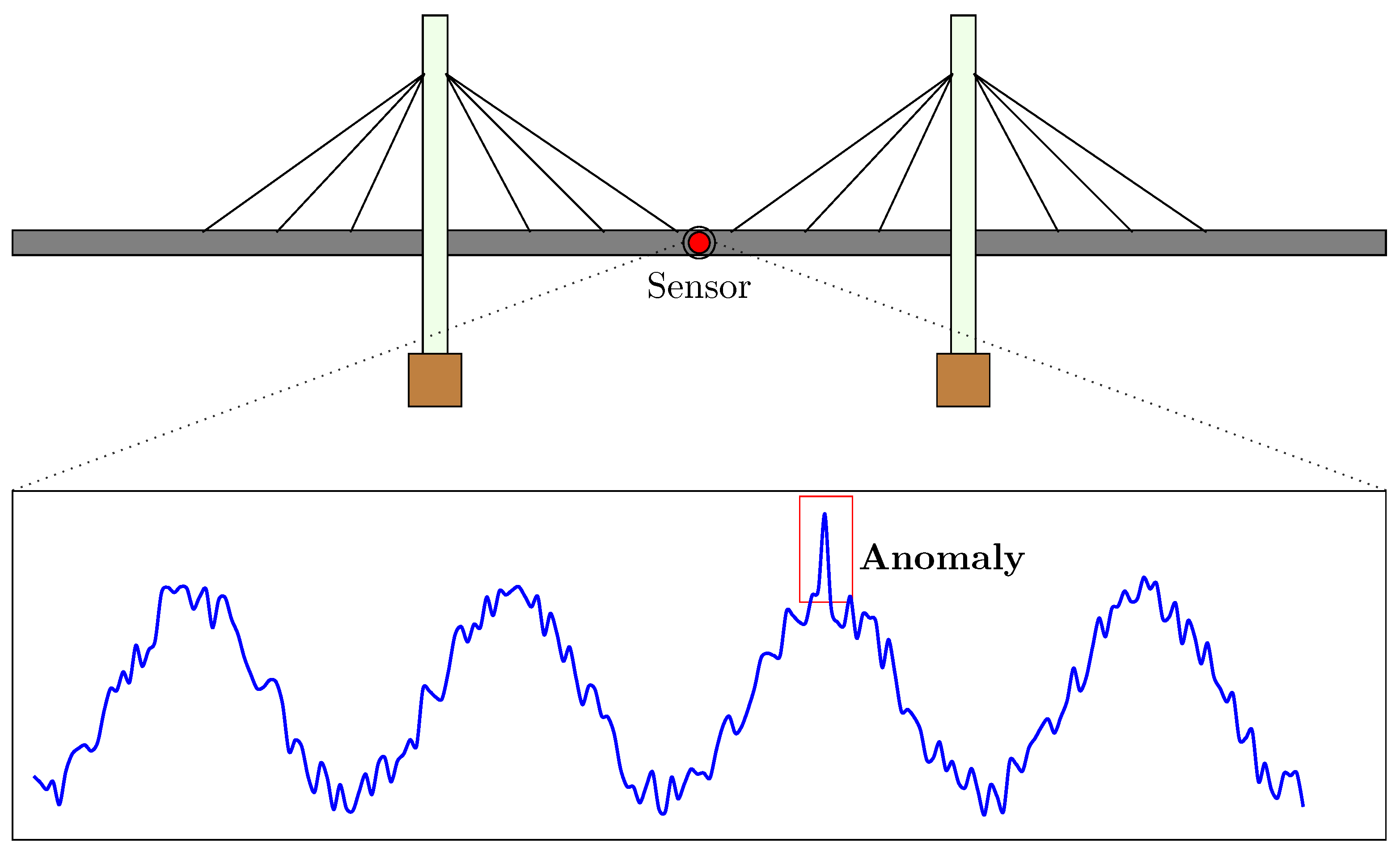
Figure 2.
A schematic representation of of a perceptron model. A weighted sum of the inputs () is passed through an activation function () to get the output ().
Figure 2.
A schematic representation of of a perceptron model. A weighted sum of the inputs () is passed through an activation function () to get the output ().
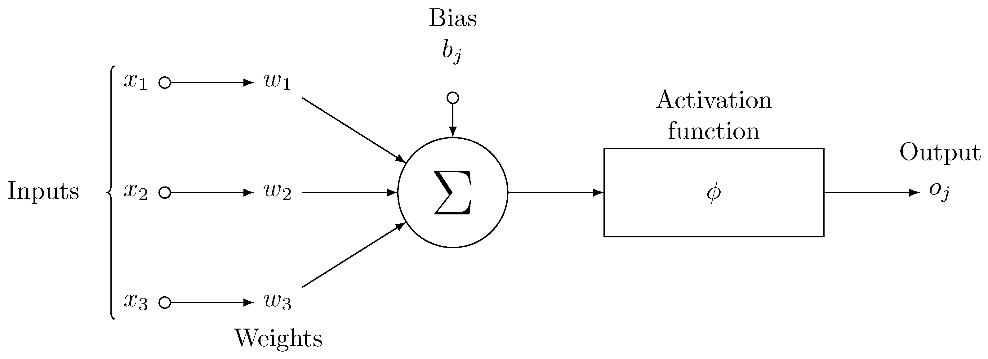
Figure 3.
A compact representation of a Feedforward Neural Network (FFNN). For simplicity, we assume , and the observation model is given by , where . The network consists of hidden layers, each containing hidden units. For any layer , the parameters between layers j and are denoted by . Adopted from Deka et al. [100].
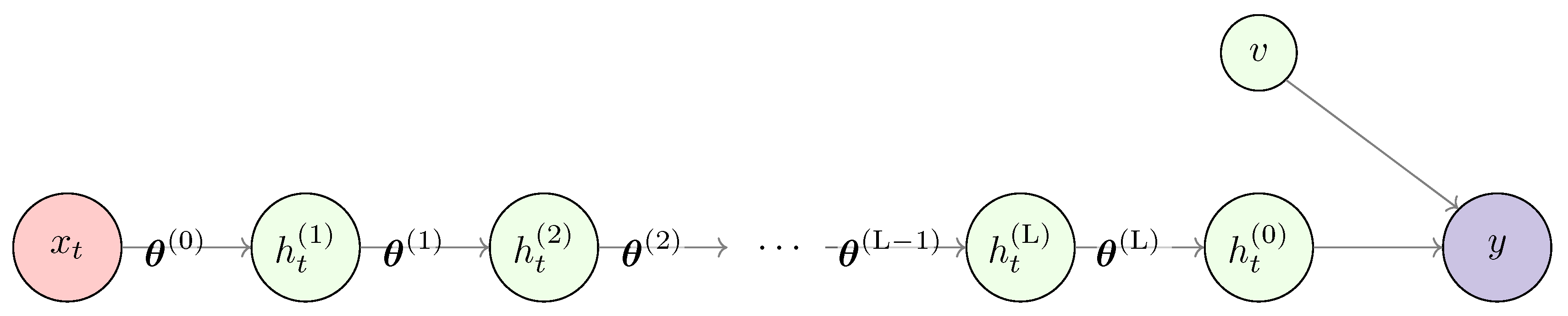
Figure 5.
Representations a rolled(a) and unrolled (b) 2-layer Deep Recurrent Neural Network (DRNN).Adapted from Vuong [110].
Figure 5.
Representations a rolled(a) and unrolled (b) 2-layer Deep Recurrent Neural Network (DRNN).Adapted from Vuong [110].
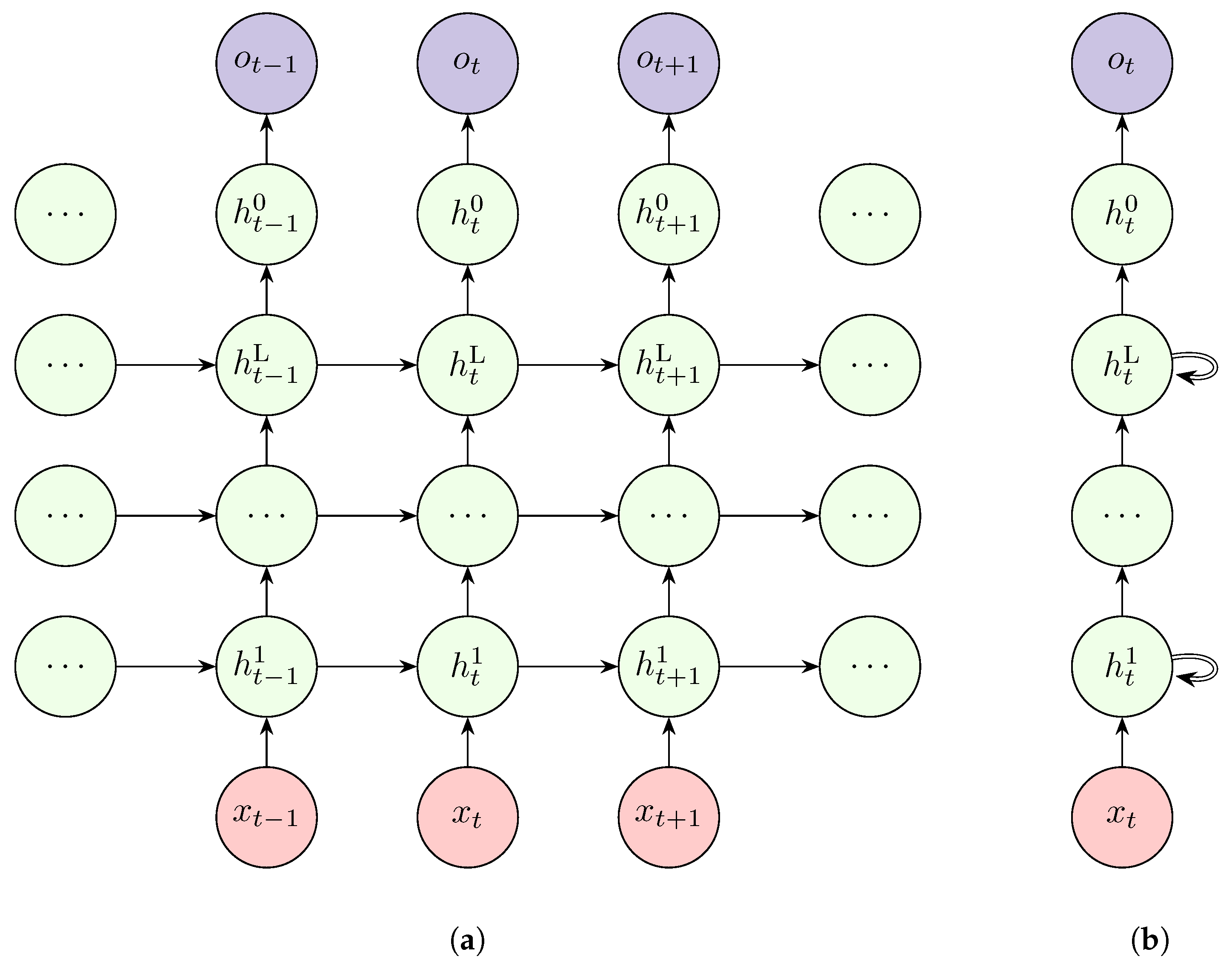
Figure 7.
Internal structure of a Long-Short Term Memory (LSTM) cell [114].
Figure 7.
Internal structure of a Long-Short Term Memory (LSTM) cell [114].
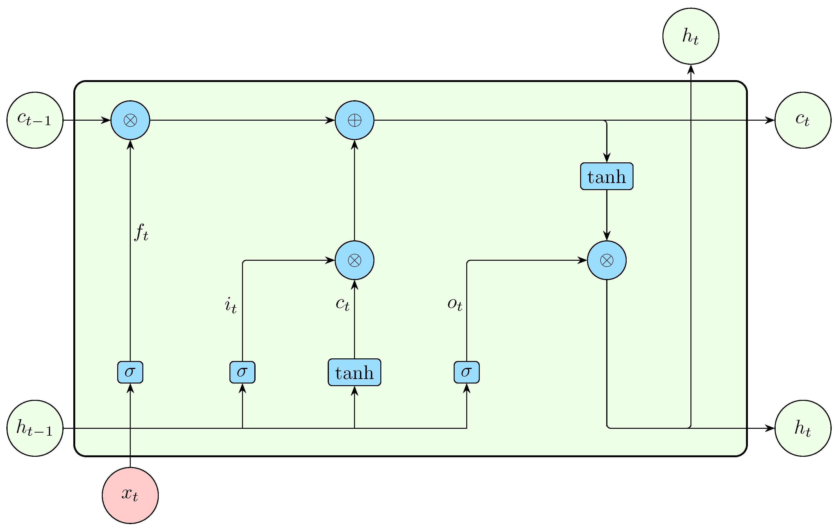
Figure 9.
Structure of physics neural time series model utilizing physics knowledge based on Simple harmonic oscillator [143].
Figure 9.
Structure of physics neural time series model utilizing physics knowledge based on Simple harmonic oscillator [143].
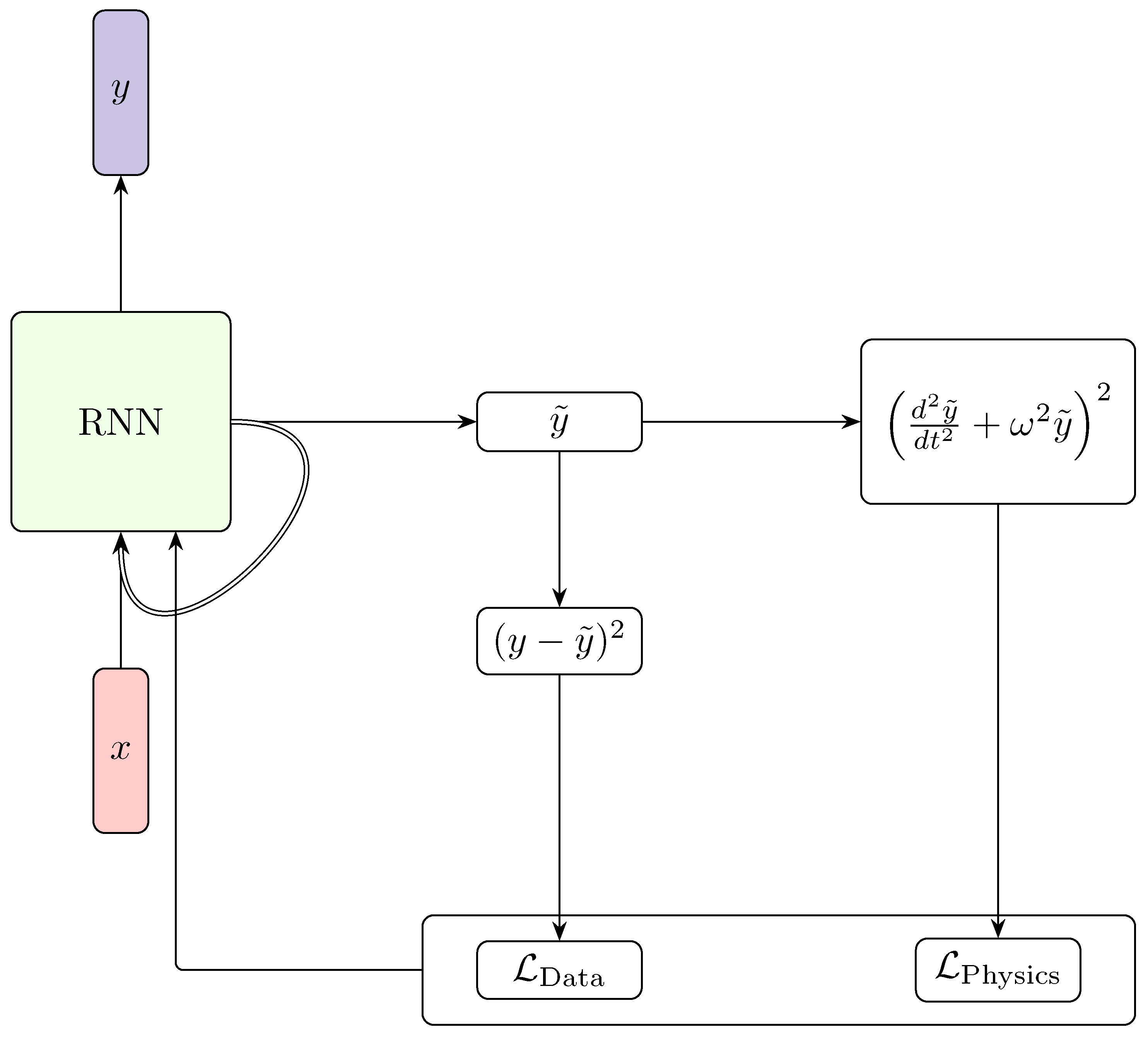
Figure 12.
Illustration of a normalizing flow transformation, adapted from Riebesell and Bringuier [167]. A simple base distribution is progressively mapped into a more complex target distribution through a sequence of invertible transformations. The process is fully reversible, allowing for inference in both forward and backward directions.
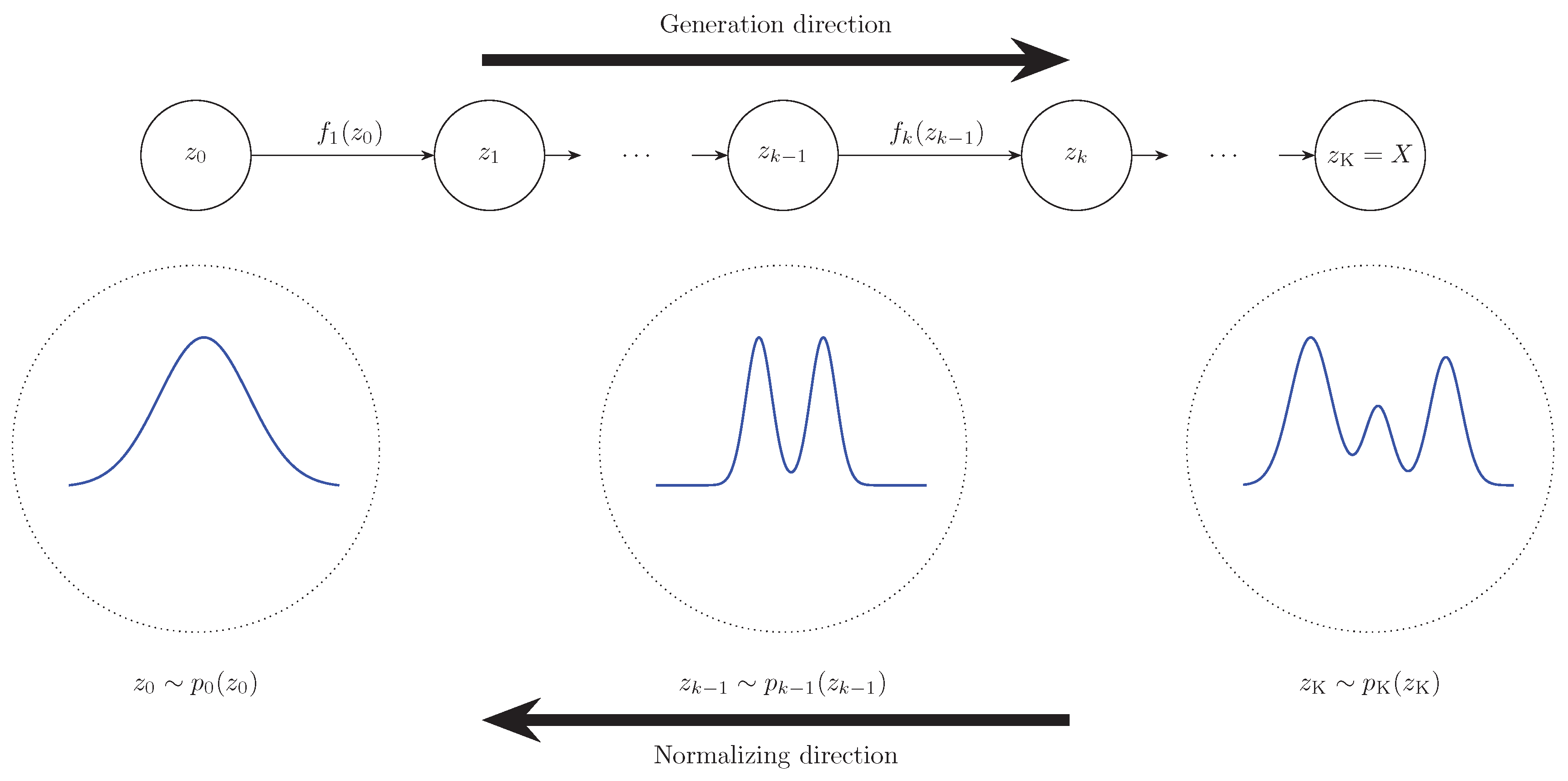
Figure 13.
A compact representation of the network in Figure 3 coupled with a directed acyclic graph (DAG) for the estimation of the variance parameter [100].
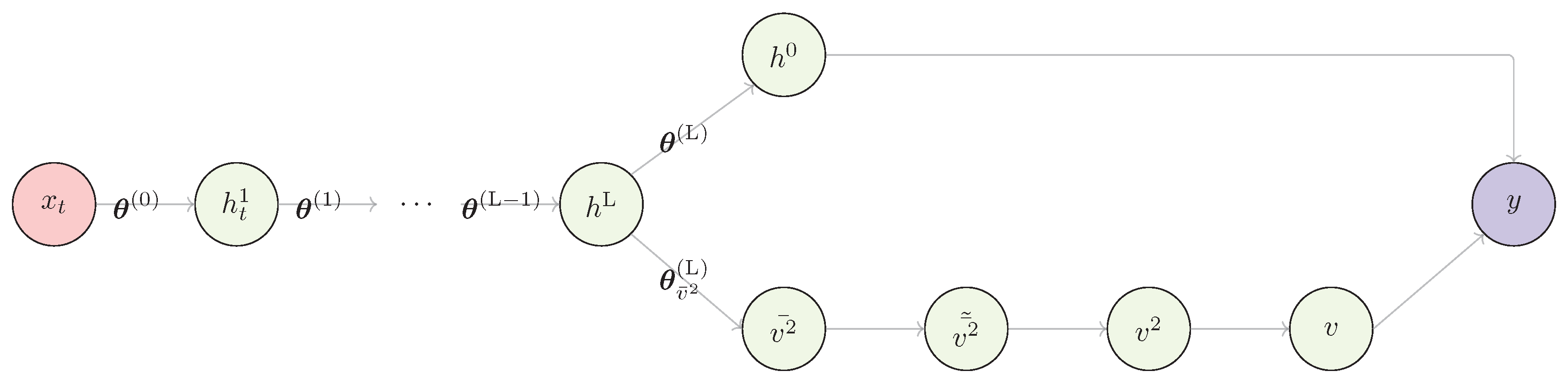
Figure 14.
PRISMA model.
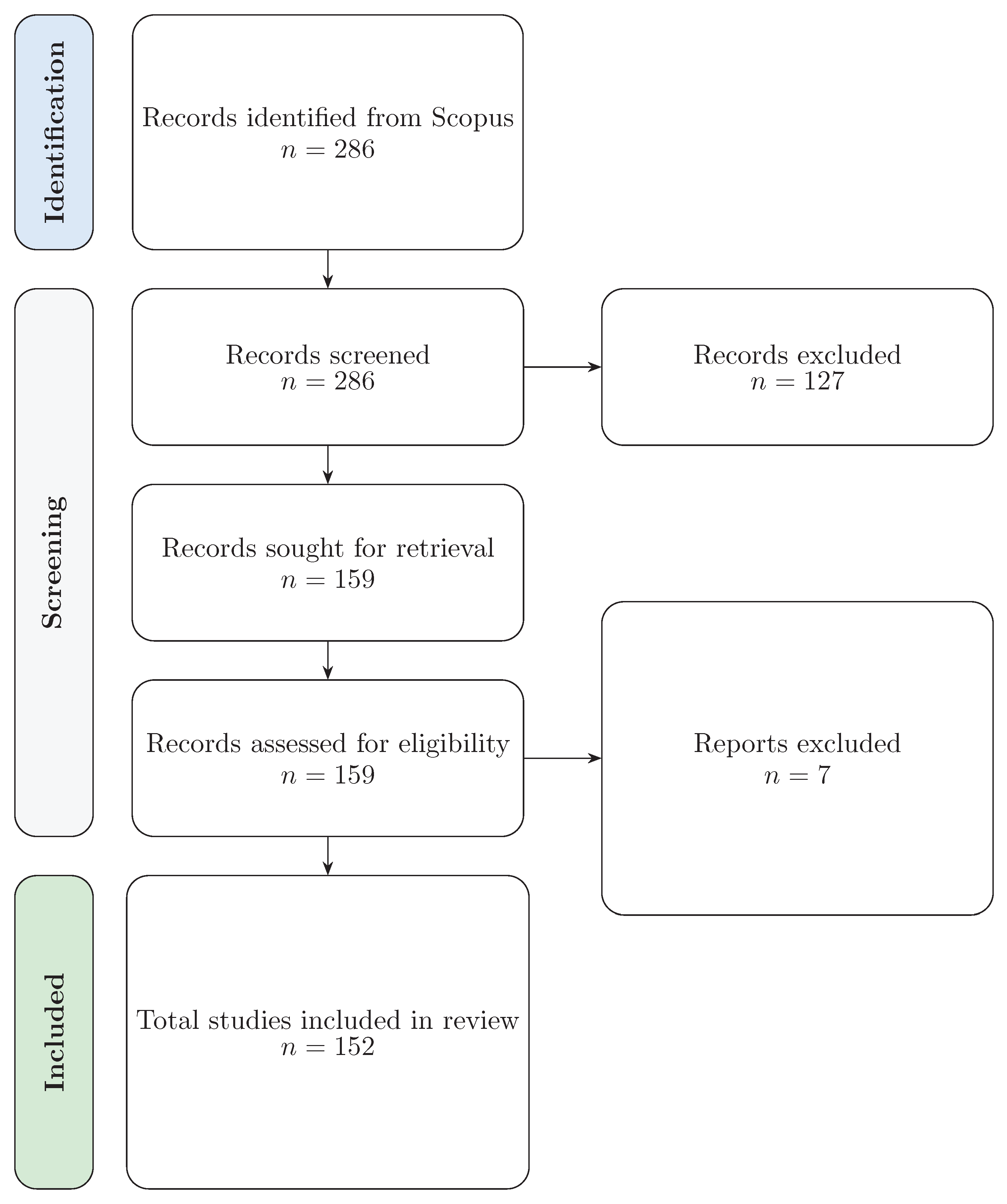
Table 1.
Common activation functions with expressions, ranges, and plots.
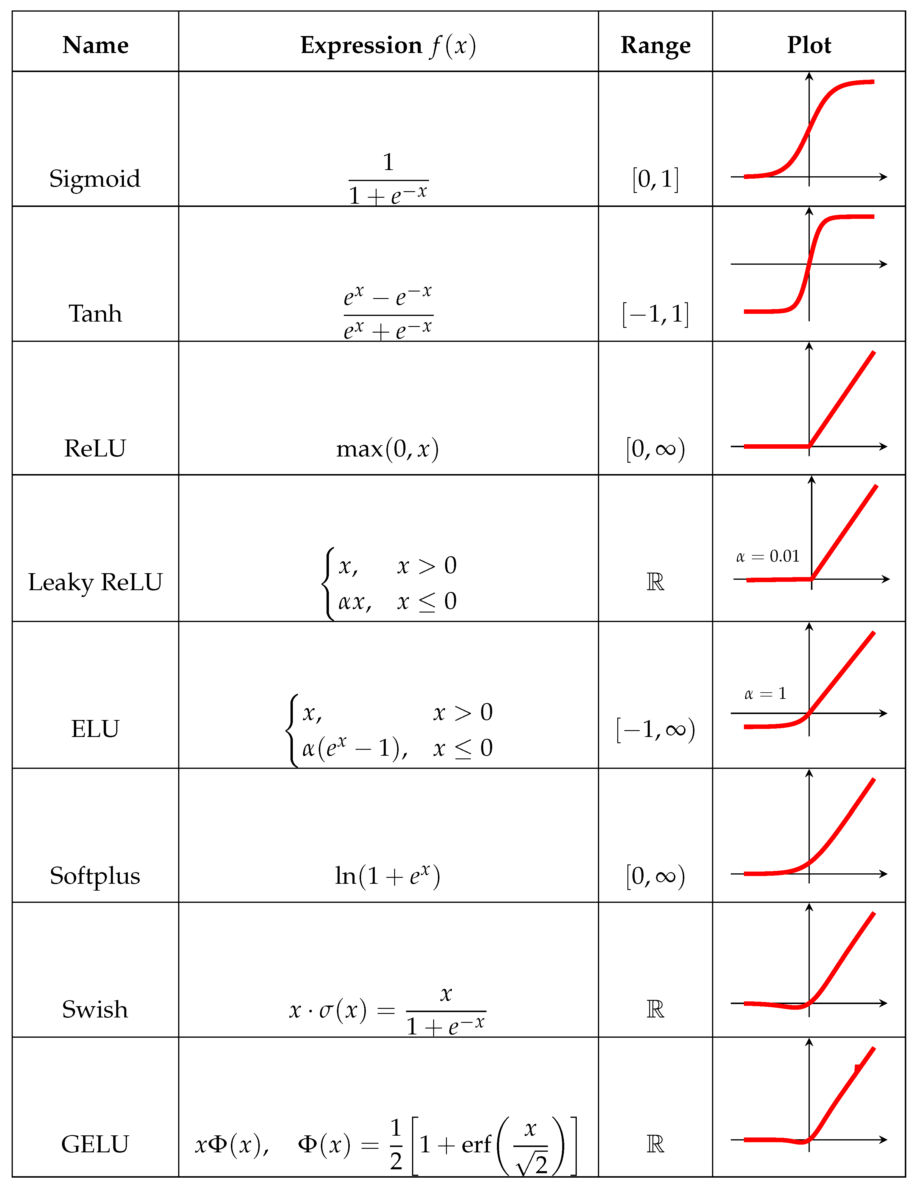
Table 3.
Comparison of Generative Models for Time Series across Structural and Functional Characteristics.
Table 3.
Comparison of Generative Models for Time Series across Structural and Functional Characteristics.
| Aspect | AE | VAE | GAN | Normalizing Flows | Diffusion Models | Autoregressive Models | Energy-Based Models |
|---|---|---|---|---|---|---|---|
| Generative Nature | Deterministic decoder | Probabilistic decoder via latent sampling | Adversarial generator-discriminator | Invertible transformation of base distribution | Gradual denoising from noise | Step-wise prediction of sequence | Energy function defines density score |
| Latent Space | Yes (fixed) | Yes (stochastic) | Often implicit | Explicit and invertible | No explicit latent space | Typically absent | Optional |
| Training Objective | MSE reconstruction | ELBO = Rec. + KL | Minimax (adversarial) | Maximum likelihood | Score-matching or ELBO variant | MLE with teacher forcing | Contrastive divergence |
| Likelihood Estimate | No | Approximate lower bound | No | Exact | Approximate (sampling) | Exact (autoregressive) | Intractable |
| Sampling Efficiency | Fast (1 pass) | Fast (1 pass) | Fast (1 pass) | Fast (invertible map) | Slow (multi-step denoising) | Fast (step-by-step) | Slow (requires MCMC) |
| Time Series Suitability | Weak (static) | Moderate with encoder/decoder | Requires temporal adaptation (e.g. RNN-GAN) | Challenging for long sequences | Promising (e.g. TimeGrad, DiffWave) | Excellent (causal modeling) | Limited or theoretical |
| Uncertainty Modeling | No | Yes | No | Limited | Yes | Limited | Yes |
| Mode Collapse Risk | Low | Low | High | Low | Low | N/A | Medium |
| Interpretability | Moderate | Moderate | Low | Moderate to high | Moderate | High | Low to moderate |
| Use in Anomaly Detection | Reconstruction error | Posterior deviation | Discriminator confidence | Log-likelihood score | Score deviation | Forecast residual | Energy score |
| Example Models | LSTM-AE, TCN-AE | VRNN, Temporal VAE | TimeGAN, C-RNN-GAN | RealNVP, MAF, Glow | TimeGrad, DiffWave | WaveNet, TransformerXL, GPT | Score-based EBMs, CPC |
Disclaimer/Publisher’s Note: The statements, opinions and data contained in all publications are solely those of the individual author(s) and contributor(s) and not of MDPI and/or the editor(s). MDPI and/or the editor(s) disclaim responsibility for any injury to people or property resulting from any ideas, methods, instructions or products referred to in the content. |
© 2025 by the authors. Licensee MDPI, Basel, Switzerland. This article is an open access article distributed under the terms and conditions of the Creative Commons Attribution (CC BY) license (http://creativecommons.org/licenses/by/4.0/).
Copyright: This open access article is published under a Creative Commons CC BY 4.0 license, which permit the free download, distribution, and reuse, provided that the author and preprint are cited in any reuse.


