1. Introduction
In the past decades, continuous casting (CC) has evolved into the most important steel casting technology. Today, about 96% is produced worldwide using this complex process [
1]. Due to this enormous throughput, increasing the reliability and efficiency of this process promises significant economical and ecological benefits. Reducing the amount of defects leads to less remelting and reworking, which is very costly in terms of time, material, machine and personnel usage. Defects in the produced steel have a variety of causes, most commonly related to the chemical composition of the steel, the cooling conditions in the mold and the secondary cooling zone as well as the mechanical condition of the casting machine.
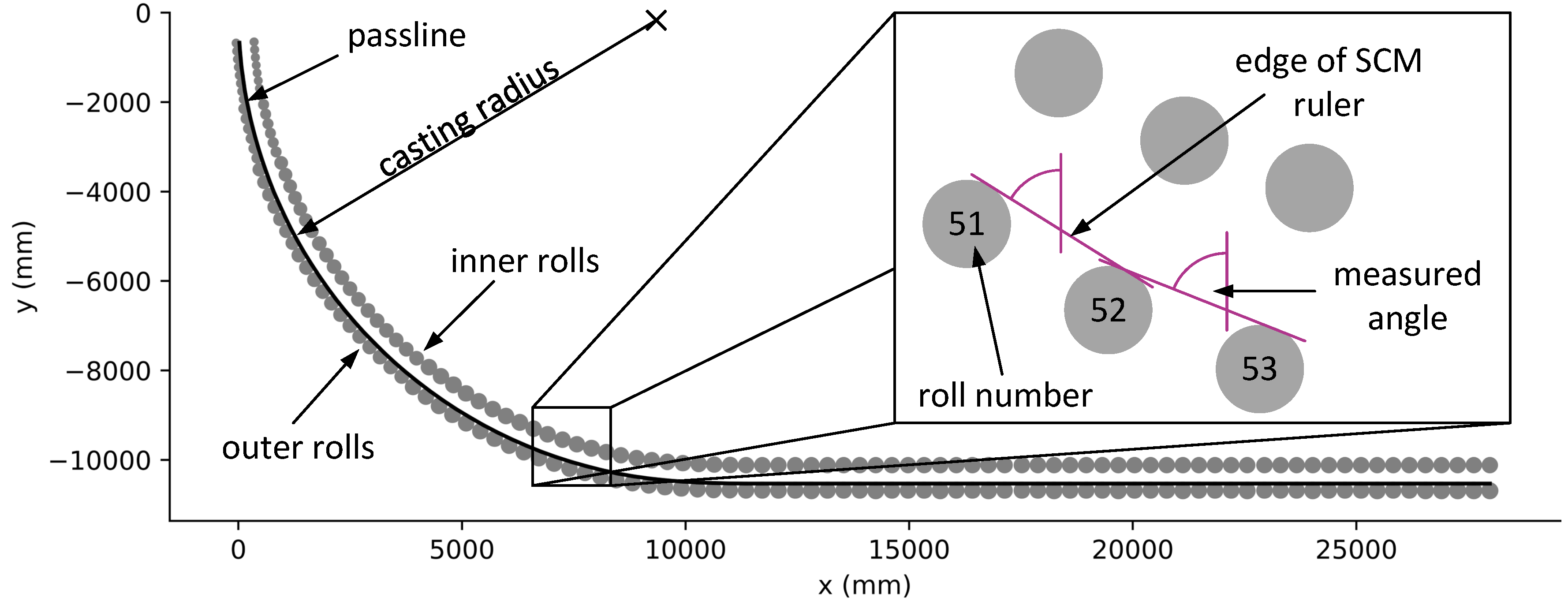
This paper focuses on the latter point, more specifically on the alignment of the rolls, that guide the strand on its way through the machine. The alignment describes how each roll position deviates from its position in the roll plan of the machine (see
Figure 1). Usually, deviations between
mm and
mm are tolerated [
2,
3]. Such tight positioning tolerances are necessary because the partially solidified strand is in a very delicate state. Misaligned rolls exert excessive force on the strand, deforming it and causing mechanical strain within the material. The solidification front within the strand is vulnerable to strains, ultimately leading to internal cracks [
1,
4,
5,
6,
7]. Maintaining the best possible alignment of the guide rolls at all times is therefore a high priority for continuous casting machine (CCM) operators.
During casting, extreme forces and temperatures act on each roll, degrading their positional accuracies over time [
6,
9,
10]. To maintain high quality production at all times, the alignment must be checked and corrected regularly. However, measuring the alignment of a CCM within the desired accuracy is not a trivial task. The rough machine environment (dirt, cooling water, electromagnetic contamination, vibrations etc.) and tight production schedules make measuring the positions of the guide rolls with the required precision very challenging. Given the tolerated position deviations, the measuring accuracy should be at least
mm.
Devices like high precision total stations or laser trackers are able to perform this task [
2,
10,
11,
12]. They achieve the desired accuracy, but they require long production pauses as well as trained and experienced personnel, which makes them unsuitable for regular maintenance.
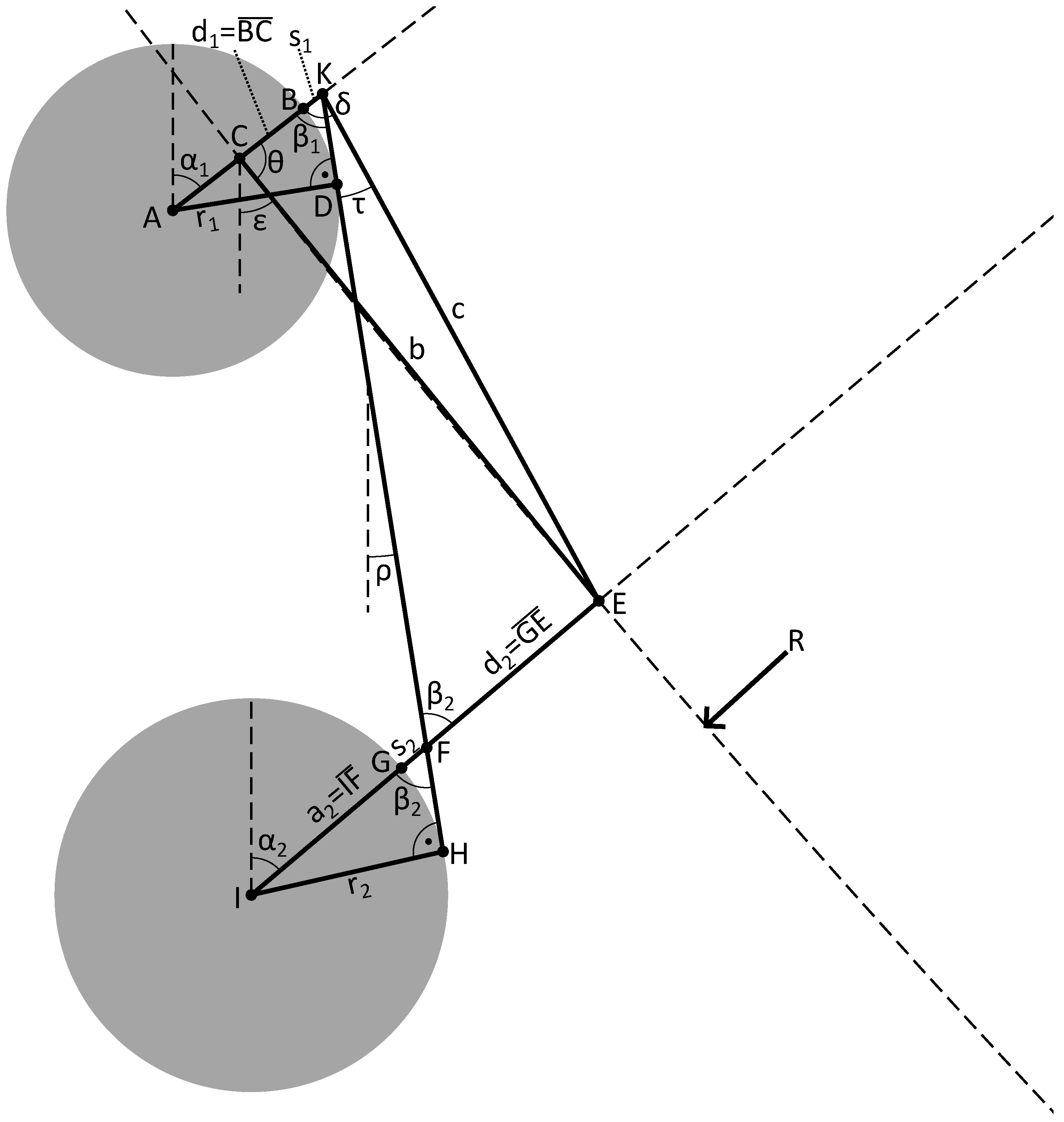
The most common tool to measure the alignment is a Strand Condition Monitoring System (SCM). SCM are measuring systems, that are integrated into the dummy bar of a CCM, which allows them to be pulled through the machine and physically touch and measure every roll. An SCM is fitted with spring loaded rulers that push against and glide over the outer rolls, while the SCM travels through the casting machine. Each time, a ruler has contact with two consecutive outer rolls, its angle is uniquely defined by the positions of the two rolls (see
Figure 1). The rulers edge forms a tangent with the circumferences of the two rolls. This tangential angle is stored for each consecutive roll pair. The result of one measurement is therefore a set of
angles, where
n is the number of outer rolls. In this paper, a CCM with
outer rolls is used as an example.
However, the tangential angles provided by an SCM are not immediately useful to a CCM operator [
13]. To determine the impact of the rolls on the strand, their absolute positions with respect to the machines coordinate system must be known. Therefore, the angles must be converted into the x-y-positions of the rolls. Since the angle measurement is conducted in a rough environment, measurement errors are not entirely avoidable. Thus, the conversion from angles to positions must be as robust as possible against errors within the angle measurements. Developing and evaluating algorithms that robustly and precisely convert the set of
angle measurements into
n roll positions represents the contribution of this work.
In the past, some researchers approached this problem, but they only considered three consecutive rolls at a time. They analyzed the measured tangential angles to retrieve positional information about the middle roll [
3,
4,
14]. However, these approaches do not compensate for the positional errors of the two neighboring rolls (see Figure 3). This paper presents a holistic solution for this unsolved challenge.
Three different approaches are described in
Section 3 and evaluated and compared in
Section 4. However, some preliminary assumptions and considerations must be taken into account beforehand.
4. Results and Discussion
In this Section, the three developed algorithms will be tested and evaluated under different conditions regarding roll position and angle measurement errors. First however, they are tested under ideal conditions to evaluate their baseline performance. These ideal conditions are:
No constant angle measurement errors.
No random angle measurement errors.
No tangential roll position errors.
No radial roll position errors.
The results of the baseline tests are shown in
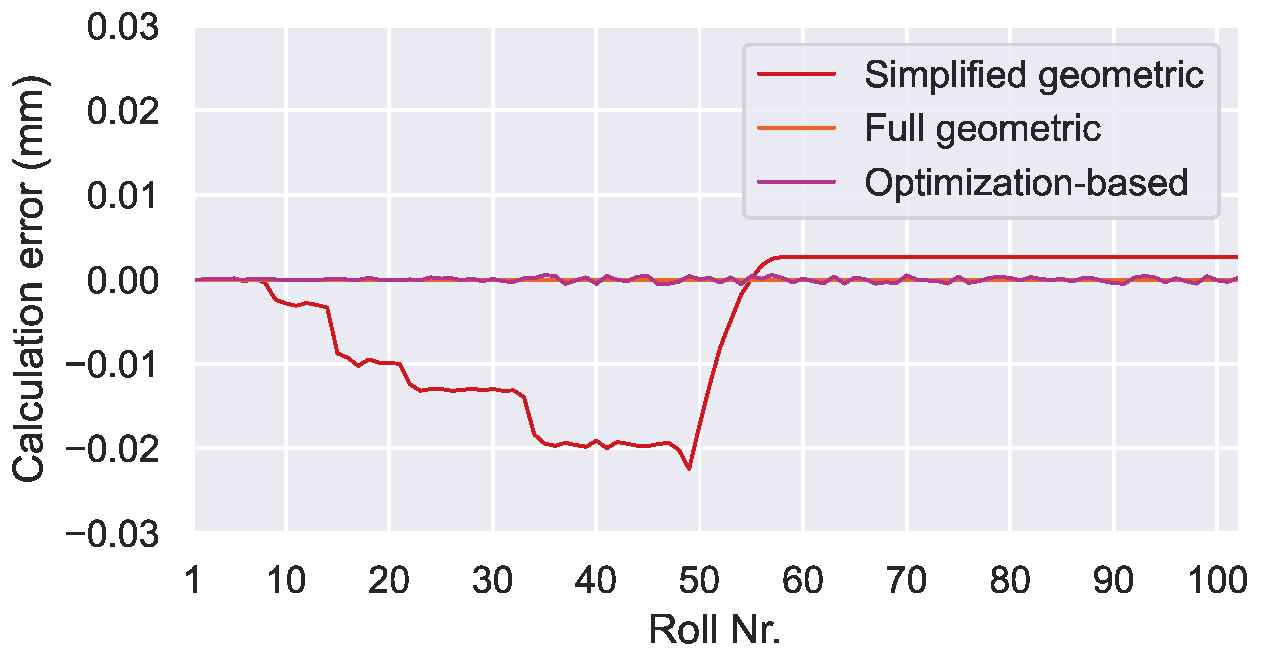
Figure 10.
The simplified geometric algorithm yields calculation errors despite the ideal conditions. This is due to the simplifying assumptions, that were made for this algorithm: neglecting the strand curvature and the varying roll diameters. The points at which the roll diameters change are visible as steps in the diagram. In the horizontal part of the machine (beginning at roll 57), both assumptions are valid, which is why this region shows no additional calculation errors. Despite these systematic calculation errors, the maximum calculation error of about mm is still small compared to the targeted accuracy, which proves the baseline functionality of the algorithm.
The full geometric algorithm shows no calculation error, as expected, since it does not make any simplifying assumptions about the machine and roll geometry.
Similar to the full geometric algorithm, the baseline performance of the optimization-based algorithm is nearly error free. However, due to the stochastic nature of this algorithm some small deviations from the ideal solution are visible. In contrast to the deterministic geometric algorithms, which always yield the same solution under the same conditions, the optimization-based algorithm shows stochastic noise in its output.
To evaluate the performance of the algorithms under non-ideal conditions, sets of roll positions with random position errors including radial and tangential components are generated. The radial components represent the target solution, which the algorithm will have to reproduce based on tangential angles. These are calculated from the roll positions using the same Equations (
21) to (
24) as in the forward function of the optimization-based algorithm. After that, artificial errors are applied to the angle values to simulate measurement errors. Two types of measurement errors can be applied: constant and random. Constant errors represent systematic measurement errors that can occur in the real world, for example with a slightly tilted or miscalibrated angle sensor. They are applied by adding a constant value to every tangential angle. Random errors occur in the real world as measurement noise or mechanical vibrations. For these, a random distribution of errors is added to the angles.
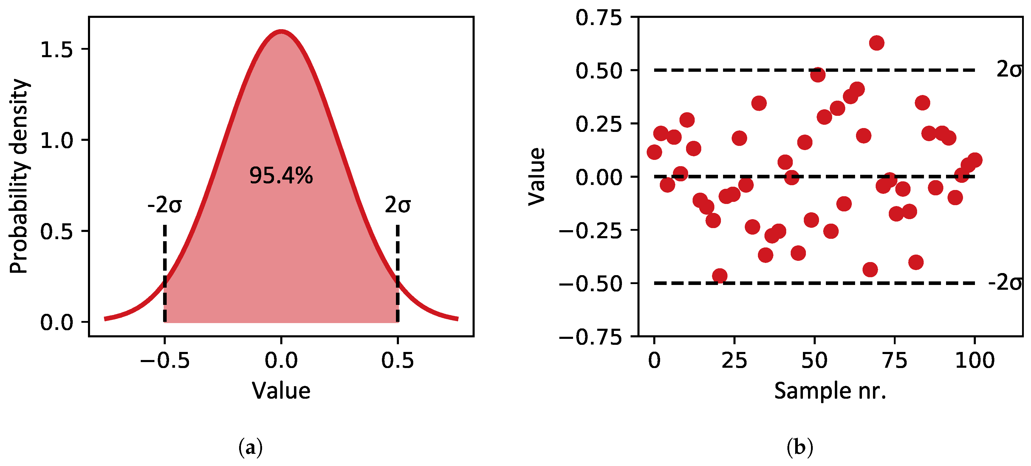
The underlying concept for random sets of values (position errors or measurement errors) is a normal distribution (see
Figure 11). In this paper, the amplitude of a random distribution is defined as two times the standard deviation of that distribution, such that 95.4% of randomly sampled values lie within that amplitude.
Each algorithm will be tested in five different experiments.
Table 2 provides an overview of the experimental conditions.
The first four experiments reveal the susceptibility of the algorithms to each of the four types of errors. In the fifth experiment, the algorithms are tested under the influence of all error types at once, which is the most realistic case. The result of the fifth experiment will determine the best performing algorithm. To keep the chapter to a reasonable size, only one error amplitude is tested in each experiment. The amplitudes represent plausible real-world values.
Every experiment will be run 100 times for each algorithm in order to capture the behavior under different random error distributions. All 100 runs are shown in the same diagram to give an impression of the average, best and worst case performances.
In Experiment 1, the influence of a radial component in the roll position errors is investigated. It is expected, that the results of this experiment are very similar to the baseline performance, since there are no measurement errors and the algorithms are designed to reproduce the radial components. However, as can be seen in
Figure 12, the performance is much worse than the algorithm’s baselines.
This result is due to the zero-mean compensation and an effect called “calculation error accumulation”. The roll position errors lead to differences between the measured tangential angles and the ideal tangential angles. The mean of this difference is not exactly equal to zero, because only about 100 values were sampled from the random distribution and because the relationship between the roll positions and tangential angles is non-linear. The compensation method interprets this as a constant error component in the angle measurement and removes it. However, because there was no measurement error in the first place, this acts like an addition of a small constant error component to the angle measurements. Even though this added error is small, the performance deteriorates significantly due to calculation error accumulation.
Calculation error accumulation is indicated by a calculation error that rises nearly linearly over the length of the machine. The results from the geometric algorithms show this behavior in
Figure 12. A constant measurement error in combination with the chain-like structure of the geometric algorithms are responsible here. At each step in the calculation chain, the constant component of the angle measurement error contributes to an error in the position calculation for the next roll. With each roll in the calculation chain, this error accumulates continuously, leading to the observed behavior. The optimization-based algorithm is much less affected, because the third term in the loss function helps to keep the predicted positions errors small. This effect was also mentioned in [
11].
To test the algorithms without the compensation, it is temporarily turned off and experiment 1 is run again. The result is shown in
Figure 13.
The simplified geometric algorithm now performs near its baseline again, with some additional noise from the random roll position errors. As expected, the full geometric algorithms returns to its error-free baseline performance. The optimization-based algorithm performs worse in this scenario, due to the third term in its loss function. The error weight was tuned to a random component in the angle measurement errors of °, which leads to a worse, but still acceptable performance.
In Experiment 2, the influence of a tangential component in the roll position errors is investigated. Since positional errors in this direction have a much lower impact on the tangential angle than radial position errors, the effect of this type of error is expected to be low.
Figure 14 shows the result of the experiment. It is apparent that random tangential position errors with an amplitude of
mm only have a small influence on the calculation accuracy. The calculation error of the geometric algorithms stays below
mm in almost every case. Starting at roll 57, the horizontal section of the plant is recognizable in all diagrams. That is expected, since tangential error components have no influence on the tangential angles in the horizontal section of the plant, when the radial components are zero. Still, some calculation error accumulation is visible for the geometric algorithms. The optimization-based algorithm seems to be especially robust against tangential errors, with a maximum calculation error of
mm. It is not affected by error accumulation and able to minimize the computation error in the horizontal section. Since the radial components of roll errors are actually zero in this experiment, the third term of the loss function has a positive impact.
In Experiment 3, the influence of a constant angle measurement error of
° is shown. Since the angle measurement error is purely constant in this experiment, the zero-mean compensation corrects it entirely. This leads to the algorithms showing their baseline performance which is not shown again. Rather, to demonstrate its effect, the compensation was temporarily deactivated for this experiment. The results are shown in
Figure 15 and demonstrate the detrimental effect of error accumulation and the necessity of the compensation. Both geometric algorithms show effetively the same result, which is an almost linearly rising calculation error. Towards the end of the machine, this error accumulates to a value close to
mm, which is unacceptable. This gave impetus to the development of the optimization-based algorithm in the first place.
The optimization based algorithm shows a much better performance, even without the zero-mean compensation. This is due to third term in the loss function, that tries to minimize the roll position. If would be set to zero, the result of the optimization-based algorithm would look like the result of the geometric algorithms. It is worth noting that between rolls 90 and 102, a small amount of the effect is also visible for the optimization-based algorithm.
This experiment demonstrates the importance of the zero-mean compensation. It shows how susceptible the geometric algorithms are to constant components in the angle measurement errors. It also becomes clear, that the additional term in the loss function of the optimization-based algorithm improves the robustness against this type of error significantly. This is important, because in the presence of a random distribution of errors, the compensation method is not able to completely remove the constant component of angle measurement errors.
In Experiment 4, all error types except random angle measurement errors are set to zero. The zero-mean compensation is activated, even though it wouldn’t show a strong effect in this experiment, since the mean of the randomly sampled angle measurement errors is near zero by definition of the normal distribution. The result is shown in
Figure 16.
Both geometric algorithms show similar performance, because the overall calculation error is much bigger than the systematic errors of the simplified algorithm. Their calculation errors mostly stay below mm. The performance of the optimization-based algorithm is significantly better, with calculation errors mostly staying below mm. No error accumulation is visible, since the error type is purely random.
Experiment 5 combines all errors from the previous four experiments. This represents the most realistic case, since the error types never occur isolated in the real world. The first four experiments were useful to explore und understand the algorithm’s behavior under different conditions. Experiment 5 will show, which algorithm works best in a real world scenario.
Figure 17 shows the result.
The results of Experiment 5 are similar, but slightly worse than Experiment 4, indicating that the influence of random angle measurement errors is dominant. Looking at the previous experiments, the reason why the other error types have minor influence becomes apparent: Radial components of roll position errors don’t have a strong influence, because the algorithms are designed to calculate those. Tangential components of roll position errors only have a small influence on the measured angles and thus on the algorithm. Lastly, constant angle measurement errors are effectively removed by the zero-mean compensation. This leaves only the random angle measurement errors to have a strong impact on the performance of the algorithms.
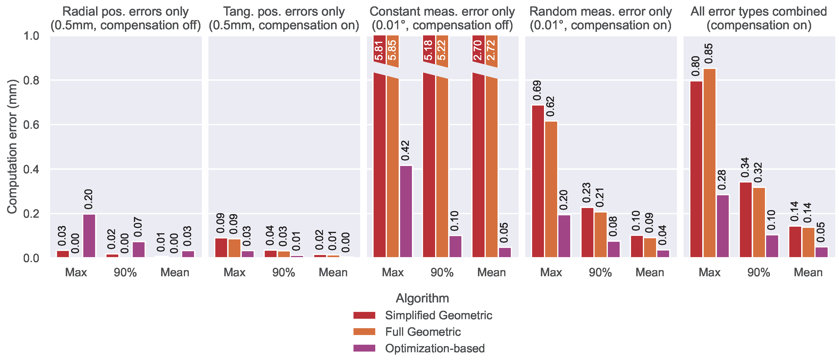
The results of all five experiments are summarized in
Figure 18.
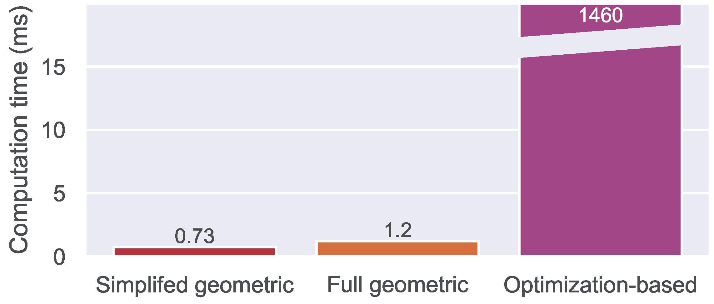
However, before the best algorithm can be determined, the computational cost must be evaluated. The average runtimes of each algorithm were measured and are shown in
Figure 19. Since both geometric approaches share the same general approach they result in a similar runtime. While the simplified approach needs a bit less than a millisecond, the full geometric algorithm takes a bit longer than a millisecond. Due to the iterative nature of the optimization-based algorithm, where all calculations are performed about 2000 times, the runtime is about 1000 times longer (
s). In the context of the application, this computation time is perfectly acceptable and it is vastly outweighed by the algorithm’s performance.
5. Conclusions
Continuously monitoring and improving the alignment condition of a CCM is a critical task to ensure a consistent and high-quality production of steel. Measuring the alignment is still a challenge today and the angle measurement data from SCM often contain systematic and stochastic errors. The contribution of this paper is the development of an algorithm that robustly and accurately converts the angle measurements into the Cartesian coordinates of the rolls with the desired accuracy of mm. Three different approaches were developed, tested and compared. The first two approaches are purely geometric and rely on trigonometry, while the third approach is based on the gradient descent optimization algorithm.
Under ideal conditions, all algorithms show very good performance. The simplifed geometric algorithm shows a computational error of around mm while the full geometric and the optimization-based algorithm yield effectively no computational error.
Five different experiments were conducted to investigate the susceptibility of the algorithms to the four error types that may occur in the real world: radial and tangential components in roll position errors as well as constant and random components in angle measurement errors. The experiments showed that the influence of roll position errors (radial and tangential) on the accuracy of the algorithms is small and remains in an acceptable range. Constant angle measurement errors on the other hand lead to large error accumulation within the geometric approaches. A constant angle measurement error as small as ° leads to computation errors of almost 6 mm. However, utilizing a zero-mean compensation method effectively mitigates this effect.
Therefore, random angle measurement errors remain as the dominant challenge for the algorithms, since these cannot be compensated nor neglected. Assuming an amplitude of ° for the random angle measurement errors, the algorithms yield mean computational errors of mm, mm and mm respectively.
The fifth experiment, which applies all four types of errors simultaneously, represents the most realistic and representative case. The results showed that the optimization-based algorithm performs on average about three times better than the geometric algorithms ( mm, mm and mm mean computational error). It is the only algorithm that reaches the desired accuracy. However, it has to be noted that the performance of the optimization-based algorithm relies on the weight factor , which depends on the amplitude of random measurement errors. This amplitude must be determined experimentally and the weight factor must be tuned for any given SCM and CCM in order to yield the shown results. Nevertheless, the gains in calculation accuracy over the geometric algorithms justify the effort.
Figure 1.
Rollplan side view [
8] and angle measurement principle. For clarity, the SCM itself is not shown. The “passline” is an imaginary line, which represents the contour of the strand backside under ideal alignment conditions. This line passes through the contact points between the outer rolls and the strands outer surface.
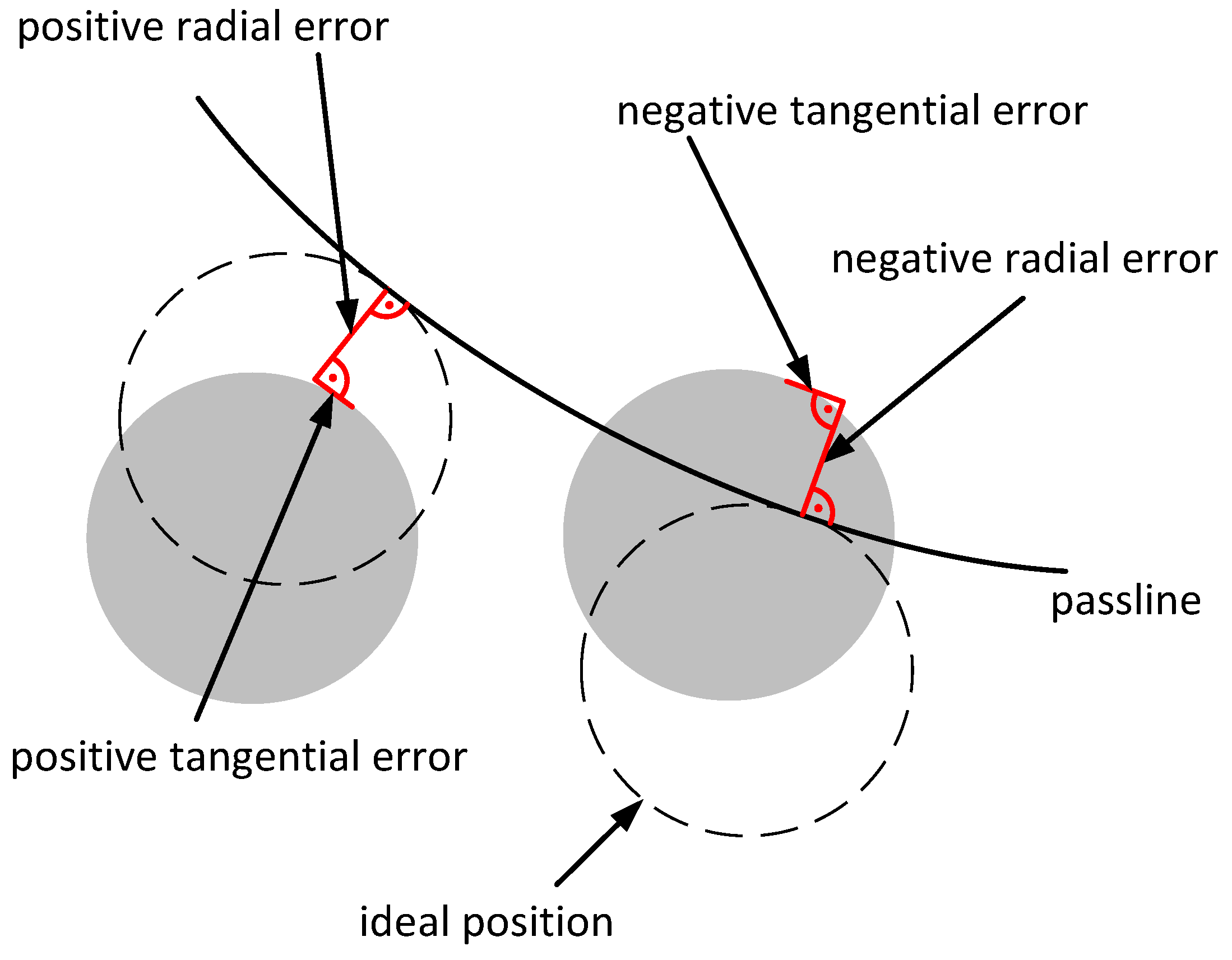
Figure 2.
Position error components and their directions. The component of the position error that is perpendicular to the passline is called “radial error” in reference to the CCMs casting radius (see
Figure 1). The error component tangential to the passline is called “tangential error”.
Figure 2.
Position error components and their directions. The component of the position error that is perpendicular to the passline is called “radial error” in reference to the CCMs casting radius (see
Figure 1). The error component tangential to the passline is called “tangential error”.
Figure 3.
Illustration of the indirect relationship between roll position errors and measured angles.
Figure 3.
Illustration of the indirect relationship between roll position errors and measured angles.
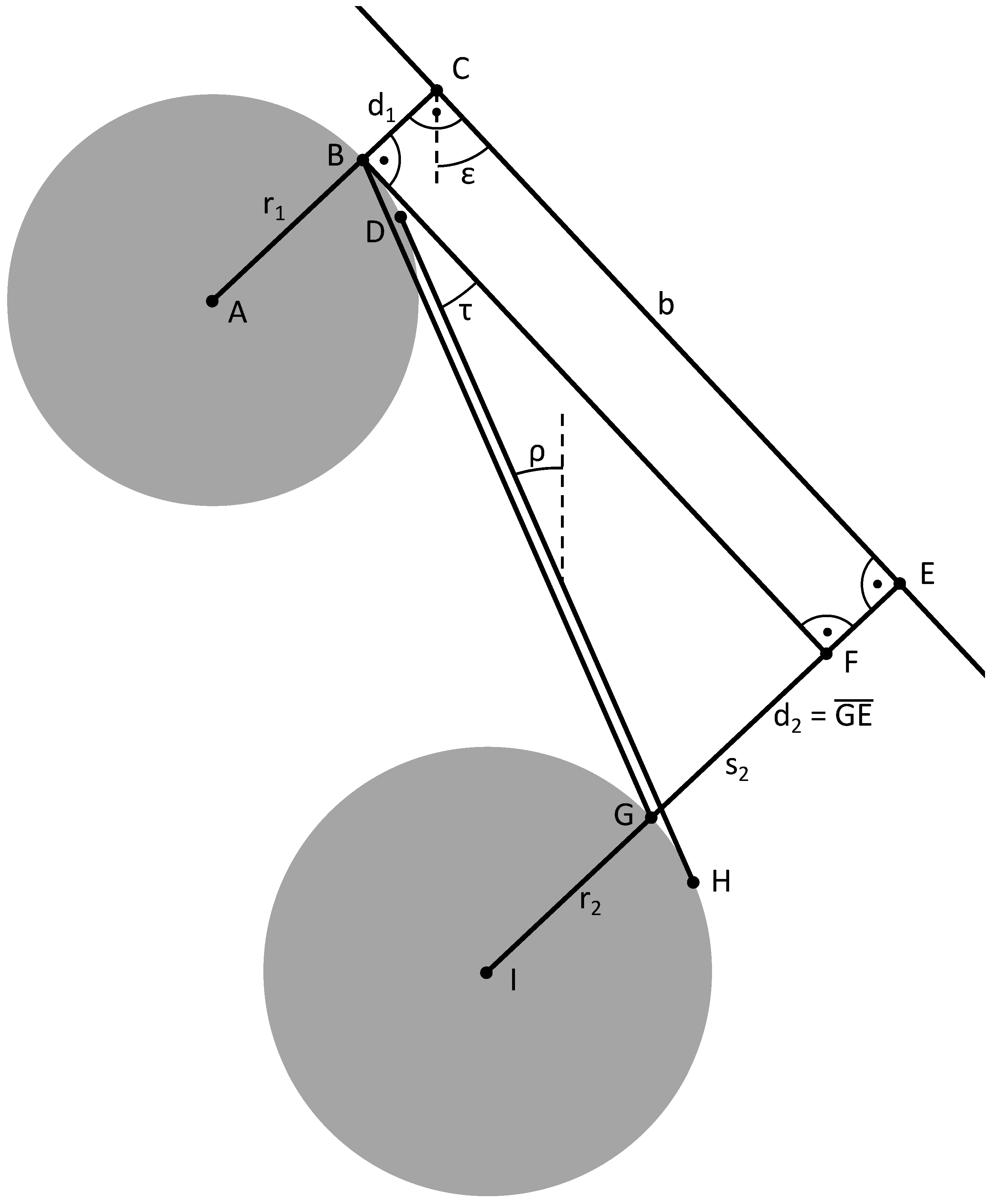
Figure 4.
Geometry of one step of the simplified geometric algorithm. Line is tangent to both rolls and represents the ruler’s edge. Due to the simplifying assumptions the passline through is a straight line and both rolls have the same radius. This leads to the four right angles and the fact that the lines and are parallel.
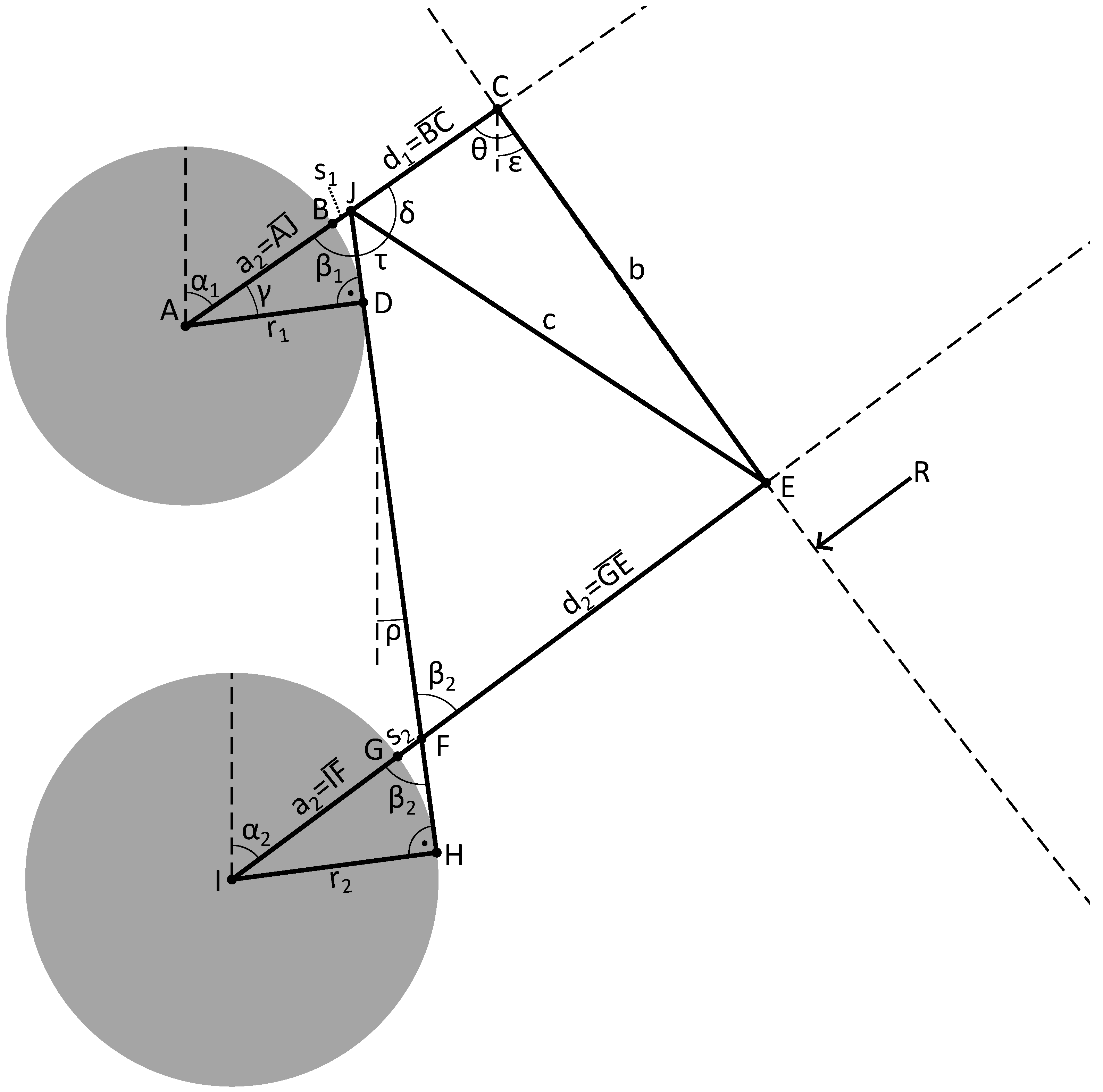
Figure 5.
Geometry of one step of the full geometric algorithm (case 1). The roll position errors in this figure are greatly exaggerated.
Figure 5.
Geometry of one step of the full geometric algorithm (case 1). The roll position errors in this figure are greatly exaggerated.
Figure 6.
Geometry of one step of the full geometric algorithm (case 2). The roll position errors in this figure are greatly exaggerated. The line is not shown for clarity.
Figure 6.
Geometry of one step of the full geometric algorithm (case 2). The roll position errors in this figure are greatly exaggerated. The line is not shown for clarity.
Figure 7.
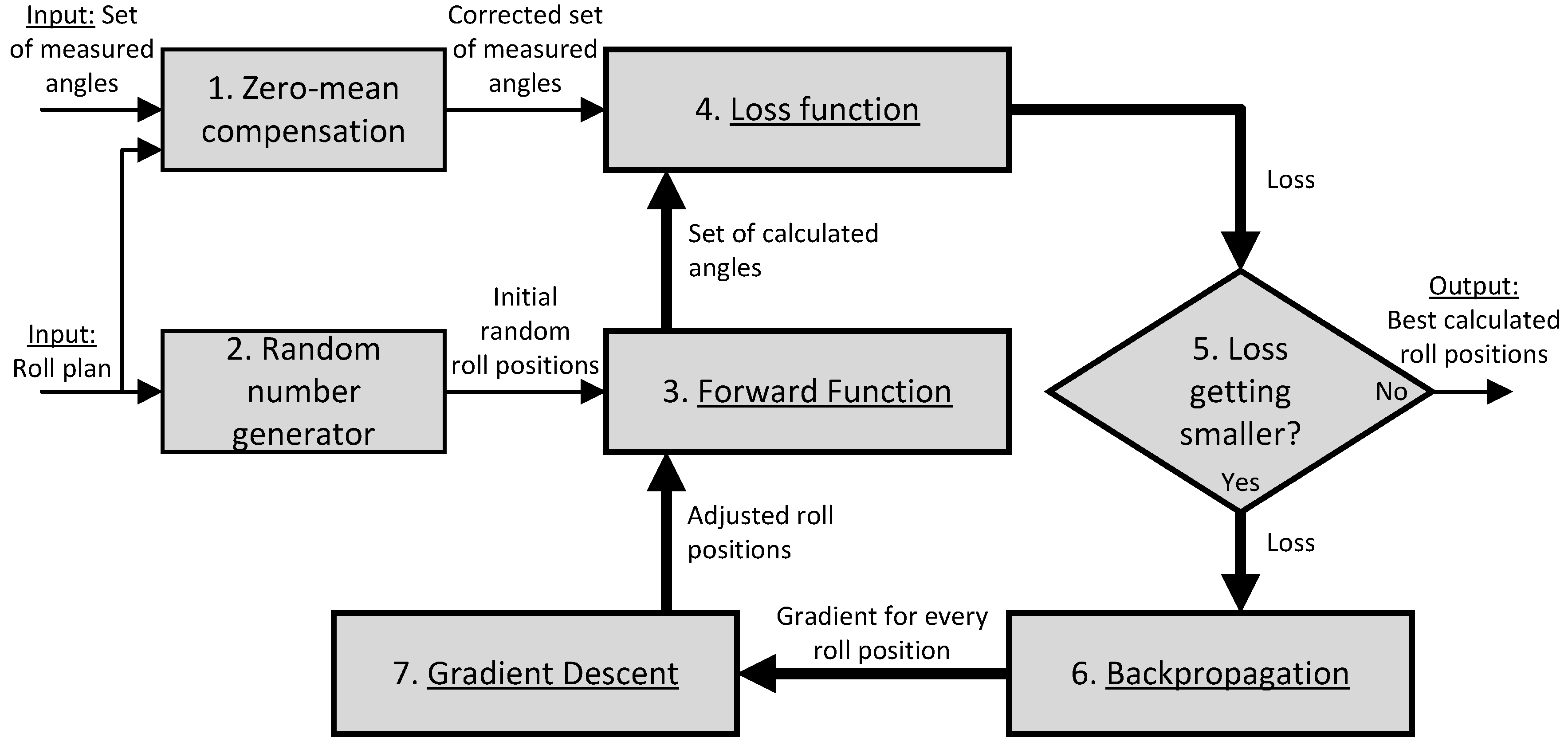
Structure of the optimization-based algorithm.
Figure 7.
Structure of the optimization-based algorithm.
Figure 8.
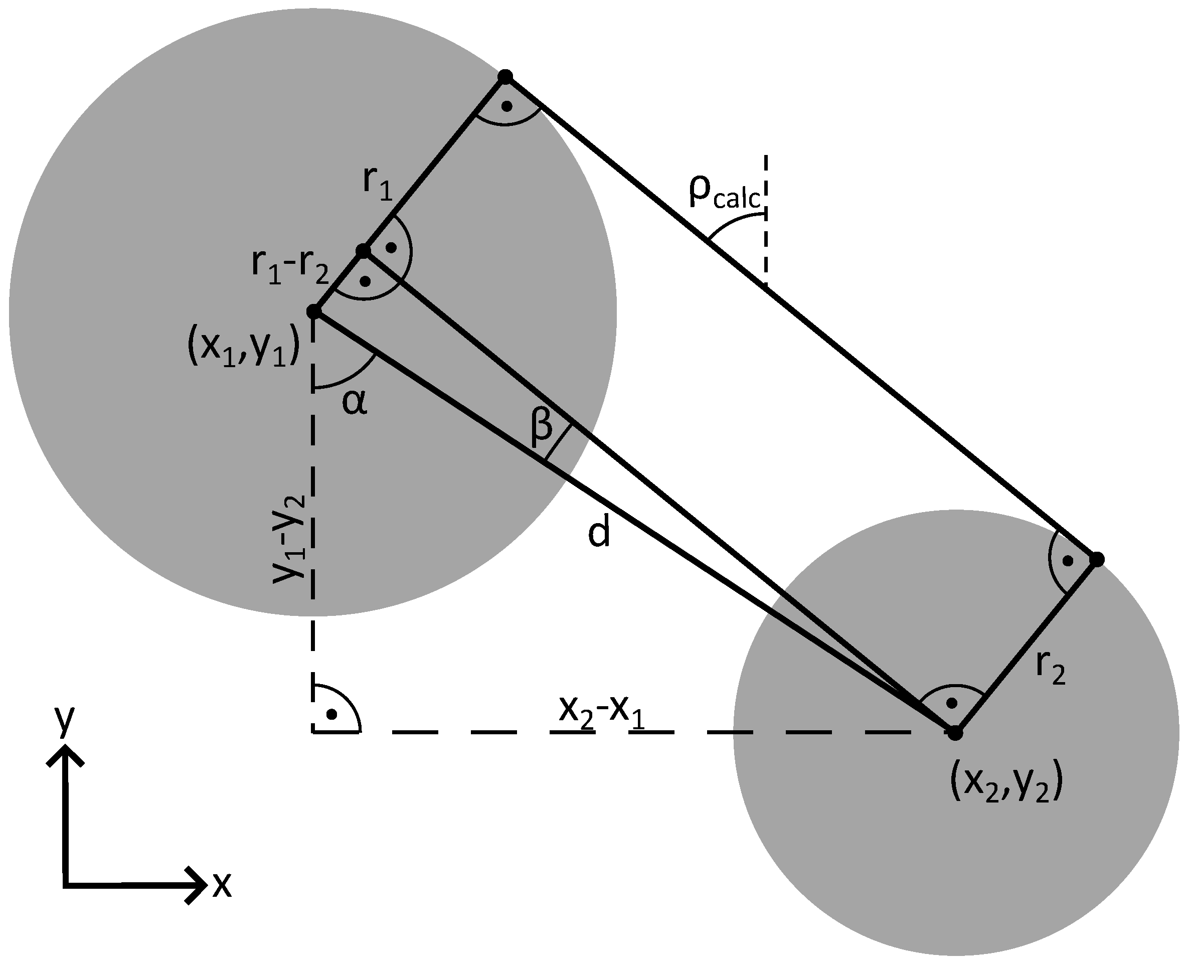
Geometry of the forward function of the optimization-based algorithm. The conversion from roll positions to tangential angles is unambiguous and straightforward.
Figure 8.
Geometry of the forward function of the optimization-based algorithm. The conversion from roll positions to tangential angles is unambiguous and straightforward.
Figure 9.
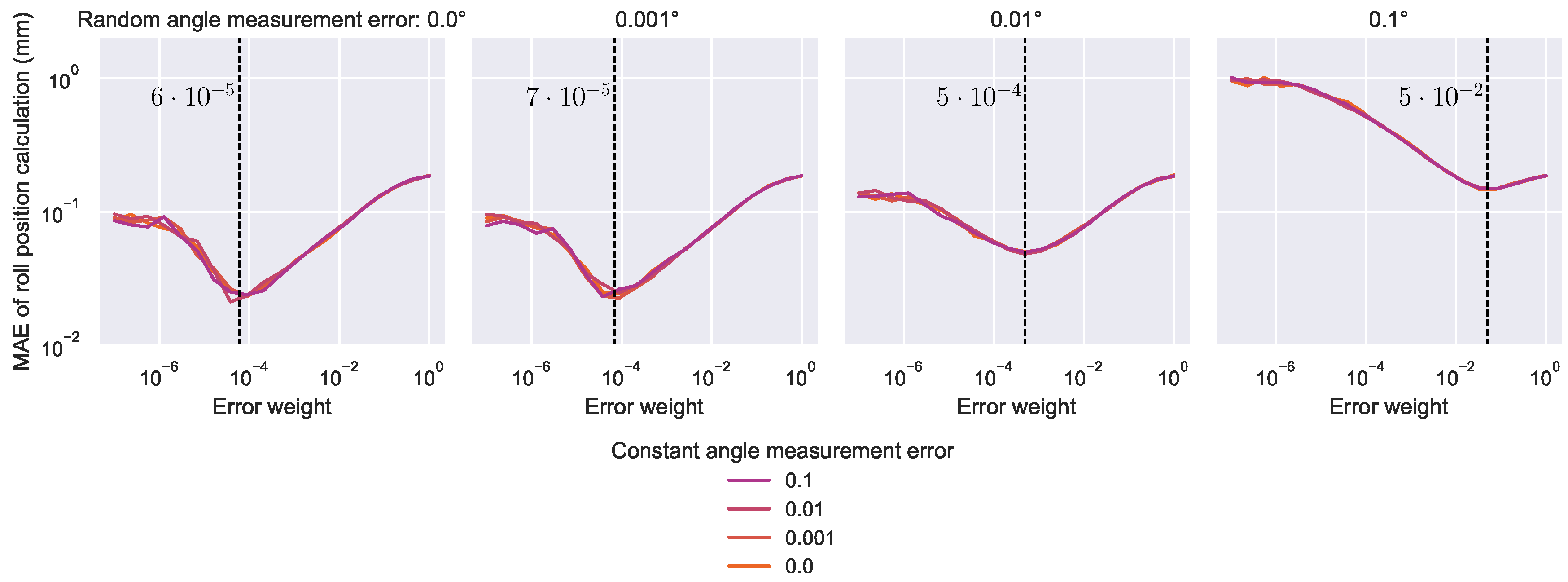
Results of the error weight optimization for the optimization-based algorithm. It is effectively independent from the amplitude of the constant measurement error. The optimal error weight for each amplitude of random measurement error is marked.
Figure 9.
Results of the error weight optimization for the optimization-based algorithm. It is effectively independent from the amplitude of the constant measurement error. The optimal error weight for each amplitude of random measurement error is marked.
Figure 10.
Baseline performances of the algorithms. The y-axis represents the difference between the calculated and the actual radial component of the roll position error. Both the full geometric and optimization-based algorithm are effectively error-free. Even the simplified geometric algorithm only deviates about mm from the target values. Since it is based on the assumption that each roll has the same diameter, changes in roll diameter cause jumps in this diagram, for example at rolls 14/15 and 33/34.
Figure 11.
(a) Normal distribution with an amplitude (two times standard deviation) of 0.5. 95.4% of sampled values will fall within this amplitude. (b) Example of 100 values sampled from that distribution.
Figure 11.
(a) Normal distribution with an amplitude (two times standard deviation) of 0.5. 95.4% of sampled values will fall within this amplitude. (b) Example of 100 values sampled from that distribution.
Figure 12.
Results of Experiment 1 with activated zero-mean compensation. The calculation errors are much worse compared to the baseline performance, because the zero-mean compensation is detrimental in this scenario.
Figure 12.
Results of Experiment 1 with activated zero-mean compensation. The calculation errors are much worse compared to the baseline performance, because the zero-mean compensation is detrimental in this scenario.
Figure 13.
Results of Experiment 1 without zero-mean compensation. As expected, the geometric algorithms performances are close or identical to their baseline performance. The optimization-based algorithm performs worse than its baseline, because its error weight is tuned to non-zero random angle measurement errors and tends to underestimate the roll position errors in this scenario.
Figure 14.
Results of Experiment 2 with zero-mean compensation.
Figure 14.
Results of Experiment 2 with zero-mean compensation.
Figure 15.
Result of Experiment 3 without zero-mean compensation. Without the compensation, the geometric algorithms suffer heavily from the influence of a constant error in the angle measurements.
Figure 15.
Result of Experiment 3 without zero-mean compensation. Without the compensation, the geometric algorithms suffer heavily from the influence of a constant error in the angle measurements.
Figure 16.
Result of Experiment 4 with zero-mean compensation. The differences between the geometric algorithms differences are insignificant compared to the influence of the random angle measurement errors. In this experiment the strengths of the optimization-based algorithm show clearly.
Figure 16.
Result of Experiment 4 with zero-mean compensation. The differences between the geometric algorithms differences are insignificant compared to the influence of the random angle measurement errors. In this experiment the strengths of the optimization-based algorithm show clearly.
Figure 17.
Results of Experiment 5 with zero-mean compensation. The result is similar to Experiment 4, suggesting that random angle measurement errors are the dominant cause for computational errors.
Figure 17.
Results of Experiment 5 with zero-mean compensation. The result is similar to Experiment 4, suggesting that random angle measurement errors are the dominant cause for computational errors.
Figure 18.
Result comparison for all experiments. Three metrics were extracted: the biggest computation error, that occured in 100 runs, the threshold under which 90% of the computation errors occured and the mean computation error. The first four diagrams illustrate the sensitivity of each algorithm regarding the four error types. In the first and third experiment the zero-mean compensation was turned off to better illustrate the algorithms properties. The rightmost diagram contains the result of Experiment 5, where all error types were combined to simulate a realistic scenario.
Figure 19.
Comparison of computation times for of each algorithm.
Figure 19.
Comparison of computation times for of each algorithm.
Table 1.
Choices for the correct case of the full geometric approach.
Table 1.
Choices for the correct case of the full geometric approach.
|
|
|
| |
|
|
|
| case 1 |
case 1 |
case 2 |
case 2 |
Table 2.
Experimental conditions to test the algorithms.
Table 2.
Experimental conditions to test the algorithms.
| |
Error amplitudes |
| |
Roll position |
Roll position |
Angle meas. |
Angle meas. |
| Nr. |
(random, radial) |
(random, tangential) |
(constant) |
(random) |
| 1 |
mm
|
0
mm |
0° |
0° |
| 2 |
0
mm |
mm
|
0° |
0° |
| 3 |
0
mm |
0
mm |
0.01°
|
0° |
| 4 |
0
mm |
0
mm |
0° |
0.01° |
| 5 |
mm
|
mm
|
0.01° |
0.01° |
