
Submitted:
29 May 2025
Posted:
29 May 2025
You are already at the latest version
Abstract
Knowledge of global radiation (Hg) is essential for regional economic development and can help guide public policies related to agricultural and energy potential. However, its availability in several Brazilian regions is still limited. This work evaluates the predictive capacity of two Machine Learning (ML) techniques, such as Multi-Layer Perceptron (MLP) and Support Vector Machine (SVM), in the estimation of Hg in 20 meteorological stations with 40 different input combinations involving insolation, air temperature, air relative humidity, photoperiod and extraterrestrial radiation. It is also compared with three empirical models based on insolation, temperature and a hybrid combination. In general, the greater the number of input variables, the better the performance of ML techniques, especially in combinations involving insolation that reduced the dispersion of estimated Hg on days with high atmospheric transmissivity and air temperature on days with low atmospheric transmissivity. The performance of SVM was better when compared to MLP in all statistical indicators. ML techniques presented better results than empirical models, and in general, the ordering of the best models in the three locations is given by: SVM, MLP and empirical models. Therefore, due to their easy implementation and generation of good results, the use of SVM models is recommended to estimate daily global radiation in the Brazilian Amazon.
Keywords:
solar radiation
; solar energy
; artificial intelligence
; SVM
; MLP
; statistical indicators
; atmospheric transmissivity.
1. Introduction
In the global context, the demand for renewable energy sources with low carbon emissions has been growing, and several countries are taking advantage of solar potential to implement photovoltaic projects. However, it is necessary to assess their viability in each region. In this context, Brazil is a country with great potential for harnessing solar energy for photovoltaic projects, as its privileged geographical location guarantees abundant incidence of global radiation (Hg) in a considerable part of its territory and throughout the year. Currently, solar energy represents around 13% of the entire Brazilian electricity matrix, being the second largest source in the country, behind only hydroelectric power [1].
There are several economic and environmental benefits that help drive the growth of this renewable energy source in Brazil. Solar energy is mainly being used as an alternative in the residential sector, as it reduces domestic electricity costs, either through thermal energy (heating water) or through the use of photovoltaic energy (generating electricity). In recent years, mainly in the Central-West and Southern regions of the Brazilian Amazon, with the consolidation and advancement of agricultural production areas, projects for photovoltaic generation plants have been established on agricultural and agro-industrial properties, aiming to supply energy to irrigation systems, warehouses and dryers, livestock facilities, farm headquarters and residences, among other rural infrastructures that require electricity.
There are several economic and environmental benefits that help drive the growth of this renewable energy source in Brazil. Solar energy is mainly being used as an alternative in the residential sector, as it reduces household electricity costs, either through thermal energy (water heating) or through the use of photovoltaic energy (generating electricity). In recent years, mainly in the Central-West and South regions of the Brazilian Amazon, with the consolidation and advancement of agricultural production areas, photovoltaic generation plant projects have been established on agricultural and agro-industrial properties, aiming to supply energy to irrigation systems, warehouses and dryers, livestock facilities, farm headquarters and residences, among other rural infrastructures that require electricity. Knowledge of global radiation incident on the surface is essential, as it is strategic and necessary information for planning various activities, such as agricultural systems, determining potential evapotranspiration [2], modeling crop growth, sizing energy systems, monitoring climate change, ecology, and construction, among others [3,4,5,6,7,8].
In the national context, due to Brazil's large territorial extension and difficulties in access, logistics, and financial and human resources for the installation and maintenance of measurement sensors, in the vast majority of Brazilian meteorological stations, global radiation is the meteorological variable with the least availability of continuous and consistent data. This reality is also observed in other regions of the world, since pyranometers, depending on the model and monitoring objective, have high acquisition costs and require periodic maintenance [7,9].
Due to the difficulty in measuring global radiation, mainly due to the costs involved in acquiring sensors [10], several studies have evaluated, over the years, different methodologies for estimating Hg, through correlation analysis with less limited meteorological variables, such as sunshine, air temperature, relative humidity, among others [5,7,8,9].
The most widespread methodologies for estimating Hg are empirical models, but recently, the number of studies evaluating Machine Learning techniques and their responses in these estimates has increased [10,11]. The first empirical model was proposed in 1924, based on linear regression between global radiation and insolation, known as the Angström-Prescott model. Still, over time, proposals for changes to this model and the generation of numerous other models emerged, with new analytical functions and input variables [7].
The increase in the processing capacity of computer systems has led to the development of new estimation methodologies, with emphasis on Machine Learning techniques [9]. Machine learning (ML) is widely used in forecasting events with non-linear characteristics, in which the learning process begins after providing a database for training, and the technique maps the patterns that will be used to predict future values [5]. Since most environmental problems have non-linear components between the dependent and independent variables due to noise, the number of studies using ML models has increased, with applications in several areas of knowledge; among them is micrometeorology, specifically the estimation of global radiation [4].
Recently, Zhou et al. [9] reviewed 232 articles on this topic and observed an exponential growth in the use of these techniques for Hg estimates between 2001 and 2020. These authors reported that there are different types of input variables, such as meteorological variables, air pollution, geographic parameters, calendar parameters, and astronomical parameters, such as extraterrestrial radiation, solar declination, zenith angle, and azimuth. According to Nawab et al. [10], the most commonly used meteorological variables for Hg estimates are air temperature, relative humidity, atmospheric transmissivity, and rainfall. Marques et al. [11] also highlight that, due to the spatial and seasonal variations of meteorological elements, it is necessary to evaluate individually, for each region, which input variables and methodologies present the best responses in Hg estimates.
The main ML techniques used to estimate global radiation are: Support Vector Machine (SVM) and Multi-Layer Perceptron (MLP) [3,5,6,11,12,13,14,15,16]. From 2000 to 2014, MLP was predominantly used in all publications, but from 2009 onwards, SVM began to be used more [17]. Both techniques are indicated for solving complex problems involving several variables and require low computational effort in processing. These techniques have been evaluated for Hg estimates in several countries, such as Brazil [13,18], Turkey [5,19,20], Spain [6], USA [6], Morocco [7,21], China [3,4,15], Iran [22], India [16], Mexico [12], Greece [14] and Ethiopia [23].
The Amazon biome covers approximately 50% of the Brazilian territory and has an area of 4,196,943 km2; it is considered the largest tropical forest in the world, and has a large carbon stock in vegetation and soil, in addition to continuously assimilating carbon dioxide (CO2) from the atmosphere through vegetation photosynthesis. In this region, surface meteorological monitoring is carried out with 72 automatic meteorological stations (AMSs) and 20 conventional meteorological stations (CMSs) belonging to the Station Network of the National Institute of Meteorology (INMET); in addition to these stations, there are also measurements of smaller time series in universities and public and private research institutions. In this region, Marques et al. [11] evaluated Hg estimates for 12 locations in the state of Amazonas, with a single combination of input variables and recommended that future work should evaluate the performance of different input combinations. Martim et al. [24] evaluated 87 empirical models to estimate global radiation in the Brazilian Amazon. They found that simple or hybrid models based on insolation and air temperature were more efficient in estimating Hg.
In general, solar radiation modeling techniques are classified based on the type of model; however, the most important issue in solar radiation modeling is model accuracy, which should be assessed using statistical indicators. Badescu [25] and Teke et al. [26] conducted extensive systematic reviews on the use of classical indicators for evaluating global radiation estimation models, which generally show errors (overestimation and underestimation), scatter, agreement, and adjustments, in percentage or energy terms. However, these statistical indicators have not been sufficient to capture differences in statistical performance when new global radiation estimation techniques are used, such as support vector machines, radial basis functions, and Bayesian neural networks.
In the context of the Brazilian Amazon, this study aimed to assess whether input variables influence the estimation of global radiation when MLP and SVM techniques and empirical models are used.
2. Materials and Methods
2.1. Study Area
The Brazilian Amazon biome has an area of approximately 4,196,943 km2 and covers the states of Acre, Amapá, Amazonas, Pará, Rondônia, Roraima and partially the states of Tocantins, Mato Grosso and Maranhão. Meteorological monitoring in the region is carried out with approximately 72 automatic weather stations (AWSs) and 20 conventional weather stations (CWSs) under the responsibility of the National Institute of Meteorology (INMET). The data are available online and can be downloaded at the electronic address (https://portal.inmet.gov.br/). In this study, data from 20 meteorological stations were used, which present concomitant measurements between automatic sensors (air temperature, relative air humidity and global radiation) and conventional sensors (insolation by heliographs), distributed in the Brazilian Amazon biome (Figure 1).
General information on meteorological stations, such as geographic location, climate classification where they are located and period of operation, is presented in Table 1. The range of the historical data series varies from 5 years for the station in the city of Óbidos to 22 years for the city of Manaus.
According to the Köppen classification, the stations are located in three climates: the tropical monsoon climate (Am) with an average monthly temperature above 18 °C, average annual rainfall greater than 1500 mm and the driest month is less than 60 mm; the humid tropical climate (Af) with an average monthly air temperature above 18 °C, average monthly rainfall above 60 mm; and the tropical savanna climate (Aw) with an average monthly temperature above 18 °C with rain in the summer [28].
2.2. Data Analysis
The daily meteorological variables selected for this study were maximum temperature (Tmax), mean temperature (Tmean), minimum temperature (Tmin), maximum relative humidity (RHmax), mean relative humidity (RHmean), minimum relative humidity (RHmin) and global radiation (Hg) obtained from the AWSs and insolation (S) obtained from the CWSs. To standardize the input data, all variables used, whether meteorological or astronomical, were integrated into the daily time scale.
In addition to the variables measured through the AWSs, two astronomical variables were also used in different combinations, extraterrestrial solar radiation (Ho) and photoperiod (So), and these variables are dependent on the time of year and latitude. They can be obtained through the equations below (Equations 1 to 5) [2,24].
where: ϕ is local latitude (in degrees); δ is solar declination (in degrees); dr is the correction factor for the eccentricity of the Earth's orbit (no-dimensionless); is the daily hour angle (in degrees); DJ represents the numerical ordering of the days throughout the year (1 ≤ DJ ≥ 365 or 366 days - leap year).
During the training and validation process of ML techniques, in addition to the availability of historical series, there is also a need to assess data quality; in this case, the implementation of strict filters must be taken into account to avoid values with reading errors or inconsistent values [9]. Therefore, the data were subjected to filters. All data from the same day were excluded if any of the following conditions were met: i) atmospheric transmissivity (Kt = Hg/Ho) above 0.85; ii) insolation ratio (S/So) greater than 1; iii) failure of hourly Hg between 9:00 and 15:00 (local time); iv) failure in the daily value of Tmax, Tmean, Tmin, RHmax, RHmean, RHmin and S.
Due to the divergence between the units representing the input variables, they were subjected to a normalization process so that the output values were normally distributed throughout their variations and between -1 and 1, and dimensionless in each variable. According to Bellido-Jiménez et al. [6] and He et al. [4], this is a common procedure in work involving ML. In the evaluation of the ML models, supervised learning was used, with the databases of each station separated into 70% for training and 30% for testing (assessment of statistical performance), systematically throughout the available historical series, to ensure the representativeness and proportionality of the periods (weeks, months and years).
2.3. Artificial Intelligence (AI) and Machine Learning (ML)
Artificial intelligence (AI) is present in several processes, with the aim of solving complex problems, as it allows the system to make decisions autonomously, according to predefined learning [10]. AI is a large area of knowledge that originated what we currently known as machine learning (ML), being divided into several techniques, which have the ability to find patterns and detect trends in non-linear systems, in problems involving classification and regression [3,5]. The most popular techniques are the Artificial Neural Network (ANN) and Support Vector Machine (SVM), and these techniques allow the processing of complex problems that involve dozens, hundreds or thousands of variables (Big Data), as is the behavior of most problems today.
2.3.1. Artificial Neural Network (ANN) - Multilayer Perceptron (MLP)
The Artificial Neural Network (ANN) was developed based on observations from studies involving models of neurons in the biological nervous system and provided the entire theoretical basis for what we know today as an artificial neural network [3,5,6,7].
The most widely used ANN is the Multi-Layer Perceptron (MLP), mainly in solving complex problems with numerous variables, which requires low computational power, enabling the modeling and analysis of extensive databases [3]. The MLP structure is subdivided into three layers: i) input layer (CE), which in the case of this study are the meteorological variables (X); ii) hidden layer (CO), where the neurons (n) are located, with the number of “n” depending on the complexity of the problem and the number of input variables; iii) output layer (CS), which represents the final result of the MLP, which in this case is the estimate of Hg [11]. All layers are interconnected by weights (W), which are numerical values that infer the importance of each input variable in the output variable, thus generating weighted connections [3,6]. Mathematically, the output value of the MLP can be modeled by Equation 6, with the multiplication of W by each variable X and the bias (β), where the sum is subjected to a non-linear sigmoid activation function (Equation 7) with output values oscillating from 0 to 1 for each neuron and k is the result in each hidden layer (Equation 8) respectively.
where: is the output variable; X is the input variable; f(k) is the sigmoid transformation function in each hidden layer; W are the weights; k k is the result in each hidden layer (Equation 8); βi is the bias in each layer.
In the training process for adjusting “W”, the iterative Back Propagation (BP) algorithm aims to minimize the loss function using gradient descent for supervised learning; this training process starts according to Equation 6, following the direct direction known as Feed-Forward, while in the reverse direction, the difference between the expected value (ME) and the output result (EST) determines the error (E) of the estimate represented in Equation 9, which serves as a reference for updating “W”, a process known as Feed-Backward; this process will be repeated iteratively until the minimum error is found by reducing the loss function or until it reaches the number of predetermined interactions for MLP learning to occur. After training, the MLP will be able to quickly and reliably predict Hg values, even if the input dataset contains noise [5].
One of the most relevant steps when working with ML techniques is defining the best hyperparameters, such as the architecture and configurations that must be determined before training [6]. In the case of MLP, it is the number of input variables, neurons, hidden layer, activation function, optimization algorithm for training, among others. In this work, through pre-tests, it was chosen to use only one hidden layer (Figure 2), with the number of neurons (n) varying according to Equation 10, given by the sum of IV (number of input variables) and OV (number of output variables). The learning rate, moment, and number of interactions used were 0.3, 0.2, and 1000 [13,18].
2.3.2. Support Vector Machine (SVM)
The Support Vector Machine (SVM) is a supervised ML technique proposed by Vapnik [29] with numerous applications in real problems, being very efficient in problems involving classification and regression [12].
As shown in Figure 3, in the SVM the hyperplane that best separates the different classes is drawn, and the data that are close to the hyperplane are known as support vectors; in this case, the hyperplane can be a straight line or plane with the function of separating the different classes [5,6]. The algorithm encompasses several activation functions, the most used being the Kernel Radial Basis Function (RBF), as it is easy to implement, efficient and can be used in multidimensional problems, that is, with a large number of input variables [3]. In the Kernel RBF function, some parameters that can change according to the input variable must be provided, such as cost (C), epsilon (ε), and gamma (γ) [12]. After several pre-tests, the following parameter values were defined (C = 100, ε = 0.001, γ = 0.3), corroborating Silva et al. [13] and Santos et al. [18]), in close regions. In Equation 11, is the output value, ω and b are known as the vector weight and bias; and as the nonlinear function.
In the Kernel RBF function described by Equation 12, the parameter represents the squared Euclidean distance in the input space and is the value determined by σ which is a free parameter. It represents the standard Gaussian noise in an infinite-dimensional space [9].
2.3.3. Structure of the Evaluated ML Models
The correct selection of input variables is an important point to be considered, as it significantly influences the predictive capacity. Several studies have evaluated the impact of different combinations on the performance of ML techniques, and in some cases, reducing the number of meteorological variables improved the predictive capacity of the ML model [4,7,19].
The input data were divided into 40 different combinations using the MLP (MLP1 to MLP40) and SVM (SVM1 to SVM40) techniques and into seven types of combination groupings, according to the input variable: I) S, So and Ho (combination 1), II) Tmax, Tmean, Tmin, So and Ho (combinations 2 to 7), III) RHmax, RHmean, RHmin, So and Ho (combinations 8 to 10), IV) Tmax, Tmean, Tmin, RHmax, RHmean, RHmin, So and Ho (combinations 11 to 24), V) Tmax, Tmean, Tmin, S, So and Ho (combinations 25 to 29), VI) RHmax, RHmean, RHmin, S, So and Ho (combinations 30 to 34), VII) Tmax, Tmean, Tmin, RHmax, RHmean, RHmin, S, So and Ho (combinations 35 to 40) (Table 2).
Both the MLP and SVM models were implemented in the open-source software Waikato Environment for Knowledge Analysis (WEKA), which has several ML libraries that prepare data, solve regression problems, classification problems, visualization, mining and association, and are intuitive and easy to execute (https://www.cs.waikato.ac.nz/ml/index.html). In WEKA, the SMOreg package was used for training and validating the SVM technique and the Multilayer-Perceptron package for the MLP technique.
2.4. Empirical Models of Hg Estimates
In addition to the Hg estimates using ML techniques, joint analyses were performed with empirical models. Martim et al. [24] evaluated 87 simplified models of Hg estimates for the same stations in this paper and indicated three empirical models, with coefficients calibrated locally (by station); in this case, the models recommended by these authors also present as input variables the insolation (S) (Equation 13), the thermal amplitude (ΔT) and the average daily temperature (Tmean) (Equation 14) and a hybrid model with thermal amplitude and insolation (Equation 15), which will be considered as EM, FAN and CHEN models, respectively throughout this paper.
2.5. Performance Analysis and Statistical Indicators
Several statistical indicators can be used to assess the statistical performance of Hg estimates [11,25,26]. Among the most used are the mean relative error (MBE - Equation 16), the root means square error (RMSE - Equation 17), the Willmott concordance index (d - Equation 18) and the coefficient of determination (R2 - Equation 19).
where: is the estimated value; is the reference value of the meteorological stations; is the average of the reference values; is the total number of observations.
Based on these indicators above, the combinations of input variables using the ML technique that generated the best Hg estimates were selected for joint evaluation with the simplified estimation models. These analyses were based on the residuals/errors ( and the sum of the quadratic residuals (SSE – Equation 20) of the adjusted models and/or ML techniques.
From the residual series Ei, bootstrap resampling techniques were applied [34,35,36], which capture the behavior of the distribution of these residuals from randomly simulated resamplings, to assess whether these residuals present similar distributions throughout their replicates. To this end, is considered to be an empirical probability distribution function of the residuals, obtained from a sample of a vector of residuals coming from an adjusted model , with a probability of occurrence of 1/N for each ; then, 10,000 random samples or bootstrap resamples are obtained, defined as a random sample of the same size N from the original residuals sample, and denoted by , which in turn will generate a new probability density function . In this way, the detailed steps of the bootstrap resampling algorithm to evaluate the closeness of the estimators (probability density function of the original residuals of the models) and (probability density function of the residuals simulated by b replicates or bootstrap resamples), can be expressed as:
- 1)
- Obtain the 10,000 residual samples of the analyzed models, , of size N, with replacement;
- 2)
- Construction of the bootstrap estimator, by constructing probability density functions of interest in each simulated bootstrap sample for residuals of the models in resamples (Equation 21);
- 3)
- Calculation of the mean () (Equation 22) and standard deviation () (Equation 23) statistics of the estimator :
- 4)
- Calculation of confidence intervals with 99% confidence for the estimate of the mean (), and with standard deviation () of the estimator , for each of the model residuals (Equation 24):
Then, the ordered theoretical quantiles of each of the residuals (simplified models and ML techniques) relative to the probability distribution function of were evaluated in the same graph; and, from this confidence interval (- Equation 24) generated by the bootstrap resampling’s, lower bands (at 0.5%, with the values of the estimates ) and upper bands (at 99.5%, with the values of the estimates ) of the 99% confidence intervals were constructed throughout the simulations of the residuals of each simplified model and ML technique. Thus, if there is a quantity greater than 1% of the residues outside these confidence bands, the residues will not be stabilized, and thus, it can be concluded that the behavior of the residues can destabilize the estimates of the evaluated models and generate bad estimates; if there is a quantity of residues less than or equal to 1% (within these confidence bands), it can be determined that these residues are stable and have a positive impact on improving the estimates, and there is an indication that the behavior of the original residues is maintained and can be considered.
For the selection of the best models, when it comes to parametric models, evaluation criteria are generally used, such as: Napierian logarithm of the likelihood function (LL – Equation 25), Akaike information (AIC – Equation 26) [37,38] and Schwarz Bayesian information (BIC – Equation 27) [39]. The interpretation of the comparison and selection of the best models based on the LL criterion occurs with the models that present the highest LL values; that is, the higher the LL, the better the model. As for the AIC and BIC criteria that penalize the adjusted parameters (k) of the models, the lower their values, the better the models.
where: is the number of observations; is the number of estimated parameters in the fitted model; is the variance of the residuals of each fitted model.
For the selection of non-parametric models, Bayesian information criteria can be used: adjusted BIC (BICc – Equation 28) [40,41], approximated WAIC (WAICa – Equation 29) [42,43] and also the generalized cross-validation criterion (GVC – Equation 30) [44,45,46].
In this case, the lower the BICc, WAICa and GVC values applied to the waste, the better the models will be. In this way, these six criteria will be evaluated in the best models chosen by the previous statistical indicators, and from these analyses, a ranking of these models can be obtained, presenting the best radiation models for each location. The works of Marques Filho et al. [47] and Elli et al. [48] use some of these model selection criteria in global radiation variables, while the research by Vasconcelos et al. [49] uses these criteria in model selection for some climate variables. Finally, the research by Zhang et al. [50] provides more details on the selection criteria used. The applications of all procedures in this section were carried out with the help of the R software [51].
3. Results
The correlations between all meteorological variables measured at the 20 stations located in the Brazilian Amazon biome were analyzed using Pearson's correlation coefficient (r) (Figure 4). Correlation values greater than 0.5 and less than -0.5 are classified as strong correlation; between 0.3 and 0.5 or -0.3 and -0.5 present a weak correlation; and below 0.3 or -0.3 present no correlation [52]. The correlation between Hg and air temperature was positive with values of 0.66, 0.56 and 0.081 for Tmax, Tmean and Tmin, respectively; with relative humidity, the correlation was inverse with values of -0.58, -0.52 and -0.23 for RHmax, RHmean and RHmin, respectively; for insolation (S), the correlation reached 0.83. Overall, the absolute value of these correlations of Hg with the other meteorological variables can be ranked in increasing order from lowest to highest correlation as |Tmin| < |RHmax| < |RHmean| < |Tmean| < |RHmin| < |Tmax| < |S|, and, with the numerical values of 0.081 < 0.23 < -0.52 < 0.56 < 0.58 < 0.66 < 0.83, respectively.
Table 3 presents the average values of the main meteorological and empirical variables to characterize the environmental conditions where the automatic (AWS) and conventional meteorological stations (CWS) are located. The climatic conditions of the Amazon biome are complex for modeling global radiation, since in this region the average rainfall is between 1,616 ± 100 and 3,205 ± 129 mm year-1, which directly interferes with the radiation and energy balance, and consequently with all other variables.
In order to understand the advances that the MLP and SVM techniques can generate in Hg estimates, comparisons were made with three empirical models that adopt the same input variables, recommended by Martim et al. [24]. Thus, the following comparisons were made: i) for insolation (S) - MLP1, SVM1 and EM model (S, So and Ho); ii) for air temperature - MLP7, SVM7 and FAN model (Tmax, Tmean, Tmin, So and Ho); iii) hybrid combinations - MLP28, SVM28 and CHEN model (Tmax, Tmin, S, So and Ho).
The predictive capabilities of the MLP (Figure 5) and SVM (Figure 6) techniques were evaluated for 40 different combinations of input variables, in 20 meteorological stations, in the Brazilian Amazon biome. Using MLP, with only S, So and Ho as input variables, the averages of R2, MBE, RMSE and “d” index were 0.7986, 0.013 MJ m-2 day-1, 1.95 MJ m-2 day-1 and 0.9394, respectively.
In the estimation possibilities when only daily air temperature data are available, the use of the combination Tmax, Tmean, Tmin, So, Ho and provides the best estimate of R2, MBE, RMSE and “d” index values of 0.6864, 0.0004 MJ m-2 day-1, 2.46 MJ m-2 day-1 and 0.8966, respectively. When only daily relative humidity data are available, the combination of RHmax, RHmean, RHmin, So, and Ho results in the best estimates. The combinations that included insolation (S) (from combination 25) improved statistical performance, regardless of the number of input variables associated with temperature and relative humidity. Notably, it is perceived that increasing the number of input variables can improve the performance of ML techniques in the estimates, which was observed with MLP; among combinations 25 and 40, the average values of R2, MBE, RMSE and “d” index were 0.84, 0.02 MJ m-2 day-1, 1.70 MJ m-2 day-1 and 0.95, respectively.
The SVM presented a predictive capacity similar to the MLP for all combinations and groupings, with better values of the R², RMSE and Willmott “d” index indicators. For example, for the combination with S, So and Ho as input variables, the values of R², MBE, RMSE and “d” were 0.8024, 0.096 MJ m-2 day-1, 1.93 MJ m-2 day-1 and 0.9421, respectively. In general, only in the relative deviations (MBE) where there is the presence of over- or underestimation, the MLP provided lower values, when compared to the SVM.
Only the three most representative combinations – which presented the best results of the statistical performance indicators (V1, V7 and V28) – were selected to evaluate the dispersion (Figure 7) between the estimated and measured values. This comparison is presented for the meteorological stations of Boa Vista (latitude 2.85º - located in the extreme north), Manaus (latitude -3.81º - central region) and Sinop (latitude -11.98º - extreme south), located in Roraima, Amazonas and Mato Grosso states, respectively. Thus, providing a comprehensive spatial analysis of the geographic and meteorological characteristics inserted in the Amazon biome and the interference of these regional conditions in the analysis of the ML modeling. In this case, global radiation (Hg) was divided according to the atmospheric transmissivity coefficient (Kt), into four intervals (highlighted in different colors): 0 ≤ Kt < 0.35 (black), 0.35 ≤ Kt < 0.55 (red), 0.55 ≤ Kt < 0.65 (green) and Kt ≥ 0.65 (blue), which correspond to the conditions of cloudy sky, partly cloudy with predominance of diffuse radiation, partly open with predominance of direct radiation and open sky, respectively, according to Escobedo et al. [53].
The predictive capacity of the MLP and SVM (Figure 8) was variable among the three meteorological stations evaluated, with greater dispersions for the Manaus station. Another important point is that the Hg estimates were closer to those measured for cloudy or clear sky conditions. The hybrid combinations, which consider the input variables insolation, temperature and relative humidity, present better Hg estimates for partially cloudy skies with a predominance of diffuse radiation. On days with high atmospheric transmissivity, there was a reduction in the spread of the estimated radiation values, both for the MLP and SVM.
There was no difference in the comparison between the empirical models and the ML techniques, with the frequency of the relative error (Figure 9) accumulated up to the value of 2.0 MJ m-2 d-1 for the EM, MLP1 and SVM1 model which was 76, 76 and 76%; FAN, MLP7 and SVM7 model with 71, 71 and 71%; and the CHEN, MLP28 and SVM28 model with 80, 82 and 83%.
Subsequently, the residues of the simplified models and of the three combinations of variables (V1, V7 and V28) for SVM and MLP were captured, in the three automatic meteorological stations (Boa Vista, Manaus, and Sinop). From their results, the graphic behaviors and their distributions and main differences throughout the series were evaluated, and these residues were simulated 10,000 times using nonparametric bootstrap techniques, in order to verify their behavior along a 99% confidence interval () in each of these residues for each of the models, at a significance level of (Figures 10 to 18 in the supplementary materials).
The analysis of the 10,000 simulations of resampling of the residues in each model indicated stable behavior for all models, as no residues were found outside the confidence bands. From the boxplots of the model residues, for most of the stations evaluated, it is observed that the smallest variations in the distributions of the residues depend on the input variables of the models (and their groupings), with the smallest variations being obtained in the following orders: i) for insolation - SVM 1, MLP 1 and EM model, (Figures 10 to 12); ii) for air temperature - SVM 7, MLP 7 and FAN model (Figures 13 to 15); iii) hybrid combinations - SVM 28, MLP 28 and CHEN model (Figures 16 to 18).
Next, descriptive analyses of the mean and standard deviation of the residues in each of these models were performed in their locations, with the aim of better understanding the variation of the residues in each of these models, as shown in Table 4. For the mean residues in increasing order, when analyzed in terms of proximity to zero, by meteorological station, the order is as follows: i) Boa Vista: simplified models < MLP < SVM; ii) for Manaus: simplified models < MLP < SVM; iii) and for Sinop, they are: MLP < SVM < simplified models. In general, in these analyses, the residue of the SVM 1 model is the one that varies the least, that is, the most stable, for the three locations.
The model selection criteria LL, AIC, BIC, BICc, WAICa, and GVC were then applied to each of these models (Table 5). In these cases, the estimates, regardless of the combination of input variables (V1, V7, or V28), the SVM presented the lowest standard deviation values in all locations, therefore presenting the smallest variations throughout its residuals.
Table 6 aims to summarize the radiation models that prevail in each of the locations, revealing an indication of the model category that appears most in each of the ordinal categories previously evaluated.
Thus, from the 6 model selection criteria evaluated for the three meteorological stations, it was observed that the order of importance of these models is in this order of SVM, MLP and empirical models, therefore showing a convergence towards the advancement of better estimates of ML models when compared with simplified models, in models of global radiation estimates in the Amazon.
Considering the ranking in Table 6, the models were compared again, considering the ranking groups of the selection criteria, aiming to choose the best model among the three evaluated for the models in the first (Table 7), second (Table 8) and third place (Table 9). Thus, in the first place of models, for the three locations it will be SVM -V28, SVM -V1 and SVM -V7 (hybrid model, with sunlight and temperature), that is, the best global model is the hybrid SVM 28.
For the cases of models in second place in Table 6, the following ordering was obtained: MLP - V28, MLP - V1 and MLP - V7 (hybrid model, with sunlight and temperature), in which case, the hybrid model MLP 28 presents the best results, and with an analogous order of models to the first place made previously. The simplified models were ranked third (Table 6). In this case, they presented variations in performance in the estimates for the meteorological stations evaluated: i) for Boa Vista and Manaus, the sequence of best performances was the CHEN, EM and FAN models; ii) for Sinop, it was the FAN, EM and CHEN models. Thus, overall, the best recommendations of the evaluated models in order of priority for use in the estimation of global radiation in the Amazon are presented in Table 10.
In all configurations, the best results were obtained by SVM and MLP, and later by empirical models; hybrid combinations of input variables (V28) or only insolation should preferably be used. The use of only air temperature data for global radiation estimates generates greater relative deviations and scattering, with under- or overestimates depending on the local/regional calibrations of the parameterized coefficients of the models.
4. Discussion
4.1. Global Radiation in Agriculture
Solar radiation can indeed serve as a predictor of agricultural productivity and food security in tropical regions. The relationship between solar radiation and agricultural productivity is complex, involving several meteorological and environmental factors such as water availability, soil quality and the impacts of climate change. The integration of solar energy into agricultural systems must be complemented by sustainable practices and policies to ensure food security. In addition, the variability in crop responses to solar radiation highlights the need for tailored agricultural strategies that consider specific regional and cultural characteristics.
The variability of solar radiation due to climatic conditions, such as cloud cover and seasonal changes, can affect its reliability, so in addition to direct measurements with pyranometers of different classes and measurement quality (depending on the sensors' construction elements), there are also different methodologies for indirect measurement (estimates). Global radiation data in different temporal partitions can be obtained by simplified statistical models [24], advanced statistical methods, machine learning, and remote sensing technologies. Numerous methodologies are being developed to improve the accuracy of estimates of global radiation and its spectral components and/or atmospheric attenuations for environmental applications and in different productive sectors, including the agricultural sector.
Recently, the combination of photovoltaic energy and crop production — often called agrophotovoltaic (APV) or agrivoltaic systems — has been suggested as an opportunity for the synergistic combination of renewable energy and food production [54,55]. This integration of solar panels with agricultural production allows for dual land use. This approach not only generates renewable energy [56], but also increases farmers’ income by enabling simultaneous crop and energy production on the same land area [57]. PV panels can be used to generate electricity for agricultural operations, especially in remote areas. This energy can power irrigation systems, crop drying processes, and other agricultural activities, reducing reliance on non-renewable energy sources [58,59].
Despite the potential benefits, there are several challenges in utilizing solar radiation data in the agricultural sector [55]. Integrating advanced technologies such as agrivoltaics and precision agriculture can require significant upfront investments and technical expertise, which can be a barrier for smallholder farmers. However, the potential of technologies to transform agricultural practices and contribute to the sustainability of this productive sector is fundamental to increasing efficiency, especially given the dependence of plant production on solar radiation. In this context, in terms of crops, global radiation data integrated with the Internet of Things (IoT) and machine learning can be used to optimize production cycles through smart technologies. By predicting more accurate levels of global radiation, farmers can make technical decisions about likely planting and harvesting dates, potential and actual productivity levels, and improve overall agricultural yields with better crop planning [60].
4.2. Machine Learning Estimates of Global Radiation
Modeling the Hg incident on the Earth's surface is complex, as this element and meteorological factors are influenced by the atmosphere, which is dynamic and composed of several elements, such as gases, dust, water vapor, and clouds [10]. These atmospheric components interact with different wavelengths of radiation and generate processes such as scattering, reflection, and absorption. According to Li et al. [61], forecasting Hg becomes more difficult as atmospheric transmissivity (Kt) decreases, i.e., cloudy/rainy days or under conditions of increased concentrations of suspended particulate matter.
Knowing that local or regional geographic conditions directly influence the seasonality and spatial distribution of meteorological variables, the selection of different input variables applied in the Hg estimate must be judicious and evaluated/calibrated for different local conditions [4]. Research involving micrometeorological modeling, both with empirical models and ML techniques, must be supported by variables with widespread measurement, low cost and with sensors that are easy to implement [62]. In this case, the greater the number of research studies developed with this theme and approach, the better the predictive capacity of ML techniques will be [9,23].
The greater the number of input variables in ML techniques, considering the same units of measurement and temporal partitions (instantaneous, hourly or daily) [such as - air temperature variations - Tmax, Tmean, Tmin, Tmax – Tmin and Tmax/Tmin], improvements in predictive capacity and statistical performance indicators are expected [6], with ML techniques being methodologies initially developed to solve complex, non-linear problems with a large number of variables [7]), as this condition is very common in tropical climate regions such as the Amazon biome, with high annual rainfall [28], which generate distinct atmospheric dynamics and can infer noise and interfere with the predictive capacity of Hg. The advantage of evaluating different combinations of input variables is that when there is no availability of a given variable, another combination can be chosen that includes the available variables and that presents a reduction in estimation errors [4].
The results showed that, depending on the combination used (Figure 5 and Figure 6), the predictive capacity of both MLP and SVM is seriously compromised, with a worsening in statistical performance. The use of RHmax and Tmin (together or separately) should be avoided, since in the day/night cycle, at the times when RHmax and Tmin occur, there is no incidence of global radiation, and, therefore, these variables present a low significant correlation with Hg. These results corroborate He et al. [4]), who evaluated the SVM in the estimation of Hg in 80 cities located in China, with different input combinations, found that, in general, the increase in the number of variables also improved the performance of the estimates, however, some variables when added did not generate better statistical performance. According to these authors, Tmin is the variable with the lowest correlation with Hg when compared to variations in air temperature (thermal amplitude, Tmax, Tmean and Tmin). For Kaba et al. [19], ML techniques, with an increase in the number of input variables, also generate improvements in Hg estimates; however, when Tmin is used in different combinations, no significant improvements are observed.
Numerically, the best statistical performances were obtained when the hybrid combination was used with all input variables (RHmax, RHmean, RHmin, Tmax, Tmean, Tmin, S, So, Ho); however, these are similar to those observed for the combinations linked only to insolation and air temperature (Tmax and Tmean). Huang et al. [22], in three different climatic conditions, with only one meteorological variable, obtained better estimates with Tmean; with the hybrid models, these same authors observed that the combination of Tmean, wind speed, relative humidity and rainfall generates good Hg estimates.
The range of statistical indicator values when analyzing the different meteorological stations is related to cloud cover and seasonality of precipitation, vegetation, and proximity to large open water surfaces, which can increase relative humidity. In addition, environmental changes caused by human actions near the measurement points (stations), such as industrial activity and fires that emit particulate matter [11], can interfere with the radiation and energy balance. When comparing the three stations at different latitudes of the Brazilian Amazon (Figure 7 and Figure 8), it is observed that the performance of ML techniques is dependent on local climate conditions.
ML techniques can estimate Hg with good accuracy in a given region, but this same technique, when used in other regions, may present worse estimates when compared to other models. This also occurs with regard to input variables, since for a given region, for example, insolation generates better estimates when compared to air temperature, and in other regions, the opposite may occur [8]. Bounoua et al. [7] showed that the statistical performance of MLP was different in five cities evaluated and related this behavior to the variability in climatic conditions and quality of measurements.
According to Agbulut et al. [5], no ML technique can perform well in all geographic and climatic regions of the world, as they are directly dependent on local conditions, data set size, geographic characteristics, and especially hyperparameters, which must be provided to the models, such as number of neurons, hidden layer, normalization of input values, and which are often subjective and require tests and evaluations of statistical indicators. For Gürel et al. [8], analyzing the parameters of the models, ML techniques, and data set for a region of interest is essential to have good estimates of any environmental variable. It is observed that the combinations of the two input variables provide better estimates of Hg, with MLP and SVM becoming limited when evaluated with few input variables, improving when the combination involving insolation, together with air temperature or relative humidity, is used. Husain & Khan [16] evaluated 12 ML models with different input combinations in a humid subtropical climate in India, and the above combinations of two variables, such as air temperature, relative humidity, and insolation, improved the performance of MLP and SVM. However, according to Nawab et al. [10], the variables that most influence the improvement of the performance of ML techniques are Tmax, Tmin, ΔT, RH, Kt, and rainfall.
The predictive capacity of Hg using SVM in a tropical climate was superior when compared to MLP, as shown in all previous analyses (Figure 9). In the literature, it is observed that this behavior is dependent on local conditions [3,5,7,12,16,20,21,52,62,63]. For Bellido-Jiménez et al. [6], MLP models are better in arid and semi-arid climates, while SVM is better in humid climates. Therefore, He et al. [4] highlight that SVM is the most widely used method to solve problems with high-dimensional and non-linear data, as it can more easily bypass data with some noise. In Brazilian conditions, in Botucatu-SP, Silva et al. [13] analyzing the correlation coefficient (r) and Willmott index (d) in the validation of SVM and MLP found for typical years with sunshine ratio (S/So) and Ho as input variables, that SVM presented R² of 0.96 and 0.98 and was better than MLP (R² of 0.924 and 0.910); however, with the inclusion of S/So, Ho, Tmax and Tmin as input variables, the statistical indicators improved significantly for both ML techniques.
Studies related to Hg estimates show that most ML techniques are more accurate when compared to empirical models, corroborating previous results [10,15]. However, this condition depends on the input variable (Figure 10), associated with the seasonal variation of precipitation and atmospheric transmissivity [61,62]. Antonopoulos et al. [14], comparing different Hg estimation methodologies and different input combinations of ML techniques for Greece, observed that the multiple linear regression (MLR) method presented the best performance with the combination of Ho, ΔT, ΔT0.5 and RHmean, followed by the empirical model of Hargreaves & Samani; in this case, both methods presented better statistical performances when compared to the artificial neural network (ANN) with the same input variables. There are advantages and disadvantages when evaluating the different methodologies, with the widespread use of empirical models enhanced by their simplicity and precision. However, they are only viable in regions with specific climate conditions, since the model parameters are fixed (coefficients) or calibrated locally.
In turn, ML models are more precise when they involve non-linear problems, extensive time series and these support dozens, hundreds or thousands of input variables; however, the optimization of hyperparameters when not taken into account can be the most significant limitation in these methodologies. Climate conditions are non-linear [23], combined with the fact that climate change is intensifying in several Brazilian regions and in other countries, and generates changes in radiation and energy balances at local and regional levels, thus demanding the need for periodic evaluations of ML techniques and recalibration of empirical models.
5. Conclusions
Increasing the number of input variables significantly improved the performance of Machine Learning techniques, with the best combination involving meteorological variables with insolation, which reduces scattering in conditions of high atmospheric transmissivity, and air temperature, which reduces the dispersion of estimated values in conditions of low atmospheric transmissivity.
Support Vector Machine (SVM) has superior performance in estimating global radiation, when compared to Multi-Layer Perceptron (MLP) and empirical models in all meteorological stations evaluated. The selection criteria demonstrate that the best models are, in this order, SVM, MLP and Empirical Models, with the SVM model presenting greater stability in generating residuals. In general, the following models are recommended for daily Hg estimates in the Amazon: SVM-V28, MLP-V28, and CHEN Model, which correspond to hybrid models that associate insolation and thermal amplitude.
This work contributes to the understanding of the complexity of the behavior of global radiation in the Amazon, and these models can contribute as another tool to be used by the agricultural and environmental sectors in Brazil, given the importance of global radiation for national agroenergy development.
Supplementary Materials
The following supporting information can be downloaded at the website of this paper posted on Preprints.org, Tables 12 to 20 – show the behavior of the residuals of the Hg estimates by the empirical models (EM, FAN and CHEN) and by the machine learning techniques SVM and MLP (V1, V7 and V28), for the meteorological stations of Boa Vista, Manaus and Sinop.
Author Contributions
Conceptualization, C.C.M. and A.P.S.; Methodology, C.C.M., D.R.B., F.T.A., J.G.R.D. and A.P.S.; Software, C.C.M., R.S.D.P. and J.G.R.D.; Validation, C.C.M., R.S.D.P., and E.T.T.; Formal analysis, C.C.M., R.S.D.P. and J.G.R.D.; Investigation, C.C.M., R.S.D.P., D.C., D.R.B., J.G.R.D. and A.P.S.; Resources, A.P.S.; Data curation, C.C.M. and A.P.S.; writing—original draft preparation, C.C.M. and A.P.S.; writing - review and editing, D.R.B., F.T.A., E.T.T., J.G.R.D. and A.P.S.; Visualization, D.R.B., F.T.A., E.T.T., J.G.R.D. and A.P.S.; Supervision, A.P.S.; Project administration, A.P.S.; funding acquisition, D.R.B., F.T.A. and A.P.S. All authors have read and agreed to the published version of the manuscript.
Funding
This research was funded by Coordenação de Aperfeiçoamento de Pessoal de Nível Superior – Brazil (CAPES) – Finance Code 001; The National Council for Scientific and Technological Development (CNPq) - Process 308784/2019-7; and the Foundation for Research Support of Mato Grosso State (FAPEMAT) - Research Project Process 0182944/2017.
Data Availability Statement
The automatic weather stations (AWS) data used in this study can be accessed by the Instituto Nacional de Meteorologia (INMET) databank website: https://bdmep.inmet.gov.br/# (accessed on 13 May 2024).
Acknowledgments
In this section, you can acknowledge any support given that is not covered by the author contribution or funding sections. This may include administrative and technical support, or donations in kind (e.g., materials used for experiments).
Conflicts of Interest
The authors declare no conflicts of interest.
References
- ABSOLAR. Associação Brasileira de Energia Fotovoltaica. Overview of solar photovoltaics in Brazil and the world. Available online: https://www.absolar.org.br/mercado/infografico/. Accessed 17 Apr 2025.
- Allen, R.G.; Pereira, L.S.; Raes, D.; Smith, M. Crop evapotranspiration guidelines for computing crop water requirements. Rome: Food and Agriculture Organization of the United Nations; 1998. 333p. Available online: https://www.climasouth.eu/sites/default/files/FAO%2056.pdf. Accessed 17 Apr 2025. (FAO Irrigation and Drainage, 56).
- Fan, J.; Wu, L.; Zhang, F.; Cai, H.; Zeng, W.; Wang, X.; Zou, H. Empirical and machine learning models for predicting daily global solar radiation from sunshine duration: A review and case study in China. Renewable and Sustainable Energy Reviews 2019, 100, 186-212. [CrossRef]
- He, C.; Liu, J.; Xu, F.; Zhang, T.; Chen, S.; Sun, Z.; Zheng, W.; Wang, R.; He, L.; Feng, H.; Yu, Q.; He, J. Improving solar radiation estimation in China based on regional optimal combination of meteorological factors with machine learning methods. Energy Conversion and Management 2020, 220, e113111. [CrossRef]
- Agbulut, Ü.; Gürel, A.E.; Biçen, Y. Prediction of daily global solar radiation using different machine learning algorithms: Evaluation and comparison. Renewable and Sustainable Energy Reviews 2021, 135, e110114. [CrossRef]
- Bellido-Jiménez, J.; Gualda, J.E.; García-Marín, A.P. Assessing new intra-daily temperature-based machine learning models to outperform solar radiation predictions in different conditions. Applied Energy 2021, 298, e117211. [CrossRef]
- Bounoua, Z.; Chahidi, L.O.; Mechaqrane, A. Estimation of daily global solar radiation using empirical and machine-learning methods: A case study of five Moroccan locations. Sustainable Materials and Technologies 2021, 28, e261. [CrossRef]
- Gürel, A.E.; Agbulut, Ü.; Bakir, H.; Ergün, A.; Yildiz, G. A state of art review on estimation of solar radiation with various models. Heliyon 2023, 9(2), e13167. [CrossRef]
- Zhou, Y.; Liu, Y.; Wang, D.; Liu, X.; Wang, Y. A review on global solar radiation prediction with machine learning models in a comprehensive perspective. Energy Conversion and Management 2021, 235(1), e113960. [CrossRef]
- Nawab, F.; Hamid, A.S.A.; Ibrahim, A.; Sopian, K.; Fazlizan, A.; Fauzan, M.F. Solar irradiation prediction using empirical and artificial intelligence methods: A comparative review. Heliyon 2023, 9(6), e17038. [CrossRef]
- Marques, A.L.F.; Teixeira, M.J.; Almeida, F.V.; Corrêa, P.L.P. Neural Networks Forecast Models Comparison for the Solar Energy Generation in Amazon Basin. IEEE Access 2024, 12, e3358339. [CrossRef]
- Quej, V.H.; Almorox, J.; Arnaldo, J.A.; Saito, L. ANFIS, SVM and ANN soft-computing techniques to estimate daily global solar radiation in a warm sub-humid environment. Journal of Atmospheric and Solar-Terrestrial Physics 2017, 155, 62-70. [CrossRef]
- Silva, M.B.P.; Escobedo, J.F.; Rossi, T.J.; Santos, C.M.; Silva, S.H.M.G. Performance of the Angstrom-Prescott Model (A-P) and SVM and ANN techniques to estimate daily global solar irradiation in Botucatu/SP/Brazil. Journal of Atmospheric and Solar-Terrestrial Physics 2017, 160, 11-23. [CrossRef]
- Antonopoulos, V.; Papamichail, D.M.; Aschonitis, V.G.; Antonopoulos, A.V. Solar radiation estimation methods using ANN and empirical models. Computers and Electronics in Agriculture 2019, 160, 160-167. [CrossRef]
- Feng, Y.; Gong, D.; Zhang, Q.; Jiang, S.; Zhao, L.; Cui, N. Evaluation of temperature-based machine learning and empirical models for predicting daily global solar radiation. Energy Conversion and Management 2019, 198, e15. [CrossRef]
- Husain, S.; Khan, U.A. Machine Learning models to predict diffuse solar based on diffuse fraction and diffusion coefficient models for humid-subtropical climatic zone of India. Cleaner Engineering and Technology 2021, 5, e100262. [CrossRef]
- Voyant, C.; Notton, G.; Kalogirou, S.; Nivet, M-L.; Paoli, C.; Motte, F.; Fouilloy, A. Machine learning methods for solar radiation forecasting: A review. Renewable Energy 2017, 105, 569-582. [CrossRef]
- Santos, C.M.; Teramoto, É.T.; Souza, A.; Aristone, F.; Ihaddadene, R. Several models to estimate daily global solar irradiation adjustment and evaluation. Arabian Journal of Geosciences 2021, 14(4), e286. [CrossRef]
- Kaba, K.; Sarigül, M.; Avci, M.; Kandirmaz, H.M. Estimation of daily global solar radiation using deep learning model. Energy 2018, 162, 126-135. [CrossRef]
- Küçüktopçu, E.; Gemek, B.; Simsek, H. Comparative analysis of single and hybrid machine learning models for daily solar radiation. Energy Reports 2024, 11, 3256-3266. [CrossRef]
- Marzouq, M.; Bounoua, Z.; Fadili, H.E.; Mechaqrane, A.; Zenkouar, K. New daily global irradiation estimation model based on automatic selection of input parameters using evolutionary neural networks. Journal of Cleaner Production 2019, 209(1), 1105-1118, 2019. [CrossRef]
- Huang, H.; Band, S.; Karami, H.; Ehteram, M.; Chau, K-W.; Zhang, Q. Solar radiation prediction using improved soft computing models for semi-arid, Slightly-arid and humid climates. Alexandria Engineering Journal 2022, 61, 10631-10657. [CrossRef]
- Woldegiyorgis, T.A.; Benti, N.E.; Chaka, N.E.; Semie, A.G.; Jemberie, A.A. Estimating solar radiation using artificial neural networks: A case study of Fiche, Oroma, Ethiopia. Cogent Engineering 2023, 10(1), e2220489. [CrossRef]
- Martim, C.C.; Paulista, R.S.; Castagna, D.; Borella, D.R.; Almeida, F.T.; Damian, J.G.R.; Souza, A.P. Daily Estimates of global radiation in the Brazilian Amazon from simplified models. Atmosphere 2024, 15(11), e1397. [CrossRef]
- Badescu, V. Assessing the performance of solar radiation computing models and model selection procedures. Journal of Atmospheric and Solar-Terrestrial Physics 2013, 105-106, 119-134. [CrossRef]
- Teke, A.; Yıldırım, H.B.; Çelik, O. Evaluation and performance comparison of different models for the estimation of solar radiation. Renewable and Sustainable Energy Reviews 2015, 50, 1097-1107. [CrossRef]
- IBGE (Brazilian Institute of Geography and Statistics). Continuous cartographic bases [database]. (2021). Available online: https://downloads.ibge.gov.br/index.htm. Accessed: 19 May 2025.
- Alvares, C.A.; Stape, J.L.; Sentelhas, P.C.; Gonçalves, J.L.M.; Sparovek, G. Köppen’s climate classification map for Brazil. Meteorologische Zeitschrift 2013, 22(6), 711-728. [CrossRef]
- Vapnik, V.N. The nature of Statistical learning theory. New York: Springer-Verlag, 1995. 201p.
- Shevade, S.K.; Keerthi, S.S.; Bhattacharyya, C.; Murthy, K.R.K. Improvements to the SMO Algorithm for SVM Regression. IEEE Transactions on Neural Networks 2000, 11(5), 1188-1193. [CrossRef]
- Elagib, N.A.; Mansell, M.G. New approaches for estimating global solar radiation across Sudan. Energy Conversion and Management 2000, 41, 419–434. [CrossRef]
- Fan, J.; Chen, B.; Wu, L.; Zhang, F.; Lu, X.; Xiang, Y. Evaluation and development of temperature-based empirical models for estimating daily global solar radiation in humid regions. Energy 2018, 144, 903–914. [CrossRef]
- Chen, R.; Ersi, K.; Yang, J.; Lu, S.; Zhao, W. Validation of five global radiation models with measured daily data in China. Energy Conversion and Management 2004, 45, 1759–1769. [CrossRef]
- Efron, B. Bootstrap Methods: Another Look at the Jackknife. In: Kotz, S., Johnson, N.L. (Eds) Breakthroughs in Statistics. Springer Series in Statistics. Springer, New York, NY. 1992. p. 569-593. [CrossRef]
- Thibshirani, R.; Leisch, F. bootstrap: Functions for the book An Introdution to the bootstrap. R package version 2019.6; 2019. Available online: https://cran.r-project.org/web/packages/bootstrap/index.html. Accessed: 27 May 2025.
- Canty, A.; Ripley, B. boot: Bootstrap R (S-Plus) functions. R package version 1.3-31 2021. https://cran.r-project.org/web/packages/bootstrap/index.html.
- Akaike, H.A. New Look at the Statistical Model identification. IEE Transactions on Automatic Control 1974, 19(6), 716-723. [CrossRef]
- Akaike, H. Information Theory and an Extension of the Maximum Likelihood Principle. In Selected Papers, Akaike. H.; Parzen, E.; Tanabe, K.; Kitagawa, G., Eds.; Springer Series in Statistics 1998, 199-213. [CrossRef]
- Schwarz, G. Estimating the Dimension of a Model. Annals of Statistics 1978, 6(2), 461-464. [CrossRef]
- Burnham, K.P.; Anderson, D.R. Model Selection and Inference: A Practical Information Theoretical Approach, 2nd ed.; Springer: New York, USA, 2002; 512p. Available online: https://link.springer.com/book/10.1007/b97636.
- Burnham, K.P.; Anderson, D.R. Multimodel Inference: Understanding AIC and BIC in Model Selection. Sociological Methods & Research 2004, 33(2), 261-304. [CrossRef]
- Watanabe, S.; Opper, M. Asymptotic Equivalence of Bayes Cross Validation and Widely Applicable Information Criterion in Singular Learning Theory. Journal of Machine Learning Research 2010, 11(12), 3571- 3594.
- Magnusson, M.; Andersen, M.R.; Jonasson, J.; Vehtari, A. Leave One Out Cross Validation for Bayesian Model Comparison in Large Data. In International conference on artificial intelligence and statistics 2020, 108, 341-351. Available online: https://proceedings.mlr.press/v108/magnusson20a.html.
- Craven, P.; Wahba, G. Smoothing noisy data with spline functions. Numerische Mathematik 1978, 31, 377-403. [CrossRef]
- Hastie T.; Tibshirani, R.; Friedman, J. The elements of statistical learning: data mining, inference, and prediction, 2009, 2. New York: Springer.
- Gueymard, C.A. A review of validation methodologies and statistical performance indicators for modeled solar radiation data: Towards better bankability of solar projects. Renewable and Sustainable Energy Reviews 2014, 39, 1024-1034. [CrossRef]
- Marques Filho, E.P.; Oliveira, A.P.; Vita, W.A.; Mesquita, F.L.L.; Codato, G.; Escobedo, J.F.; Cassol, M.; França, J.R. Global, diffuse and direct solar radiation at the surface in the city of Rio de Janeiro: Observational characterization and empirical modeling. Renewable Energy 2016, 91, 64-74. [CrossRef]
- Elli, E.F.; Olivoto, T.; Schmidt, D.; Caron, B.O.; de Souza, V.Q. Precision of Growth Estimates and Sufficient Sample Size: Can Solar Radiation Level Change These Factors? Agronomy Journal 2018, 110, 155-163. [CrossRef]
- Vasconcelos, J.C.S.; Lopes, S.A.; Arenas, J.C.C.; da Silva, M.F.G. Flexible regression model for predicting the dissemination of Candidatus Liberibacter asiaticus under variable climatic conditions. Infectious Disease Modelling 2025, 10, 60-74. [CrossRef]
- Zhang, J.; Yang, Y.; Ding, J. Information criteria for model selection. Wiley Interdisciplinary Reviews (WIREs) Computational Statistics 2023, 15, 1-27, e1607. [CrossRef]
- R Core Team. R: A Language and Environment for Statistical Computing. R Foundation for Statistical Computing 2025, Vienna, Austria. Available online: https://www.R-project.org/. Accessed: 27 May 2025.
- Liu, F.; Wang, X.; Sun, F.; Wang, H. Correct and remap solar radiation and photovoltaic power in China based on machine learning models. Applied Energy 2022, 312, e118775. [CrossRef]
- Escobedo, J.F.; Gomes, E.N.; Oliveira, A.P.; Soares, J. Modeling hourly and daily fractions of UV, PAR and NIR to global solar radiation under various sky conditions at Botucatu, Brazil. Applied Energy 2009, 86(3), 299-309. [CrossRef]
- Weselek, A.; Ehmann, A.; Zikeli, S.; Lewandowski, I.; Schindele, S.; Högy, P. Agrophotovoltaic systems: applications, challenges, and opportunities. A review. Agronomy for Sustainable Development 2019, 39, e35. [CrossRef]
- Wydra, K.; Vollmer, V.; Busch, C.; Prichta, S. Agrivoltaic: solar radiation for clean energy and sustainable agriculture with positive impact on nature. In: Aghaei, M.; Moazami, A. (Eds). Solar radiation – enabling technologies, recent innovations, and advancements for energy transition. Intechopen, 2024. [CrossRef]
- Jain, S. Agrivoltaics: the synergy between solar panels and agricultural production. Darpan International Research Analysis 2024, 12(3), 137-149. [CrossRef]
- Giri, N.C.; Mohanty, R.C.; Shaw, R.N.; Poonia, S.; Bajaj, M.; Belkhier, Y. Agriphotovoltaic systems to improve land productivity and revenue of farmer. In: IEEE Global Conference on Computing, Power and Communications Technologies 2022, 1-5, . [CrossRef]
- Adeyanju, O.O.; Nabage, O.H.A.; Orimaye, O.S. Solar energy meteorology in agriculture – an X-ray of solar irradiance. International Journal of Current Science Research and Review 2022, 5(7), 2689-2697. [CrossRef]
- Yajima, D.; Toyoda, T.; Kirimura, M.; Araki, K.; Ota, Y.; Nishioka, K. Estimation model of agrivoltaic systems maximizing for both photovoltaic electricity generation and agricultural production. Energies 2023, 16(7), e3261. [CrossRef]
- Ghosh, S.; Sarkar, A.; Mitra, A.; Das, A. Smart cropping based on predicted solar radiation using IoT and machine learning. In: IEEE International Conference on Advanced Trends in Multidisciplinary Research and Innovation 2020, 1-5. [CrossRef]
- Li, Y.; Wang, Y.; Qian, H.; Goa, W.; Fukuda, H.; Zhou, W. Hourly global solar radiation prediction based on seasonal and stochastic feature. Heliyon 2023, 9(9), e19823. [CrossRef]
- Jia, D.; Yang, L.; Lv, T.; Liu, W.; Gao, X.; Zhou, J. Evaluation of machine learning models for predicting daily global and diffuse solar radiation under different weather/pollution conditions. Renewable Energy 2022, 187, 896-906. [CrossRef]
- Nematchoua, M.K.; Orosa, J.A.; Afaifia, M. Prediction of daily global solar radiation and air temperature using six machine learning algorithms; a case of 27 European countries. Ecological Informatics 2022, 69, e101643. [CrossRef]
Figure 1.
Location map of the 20 automatic and conventional meteorological stations distributed throughout the Amazon biome. Database: IBGE [27].
Figure 1.
Location map of the 20 automatic and conventional meteorological stations distributed throughout the Amazon biome. Database: IBGE [27].
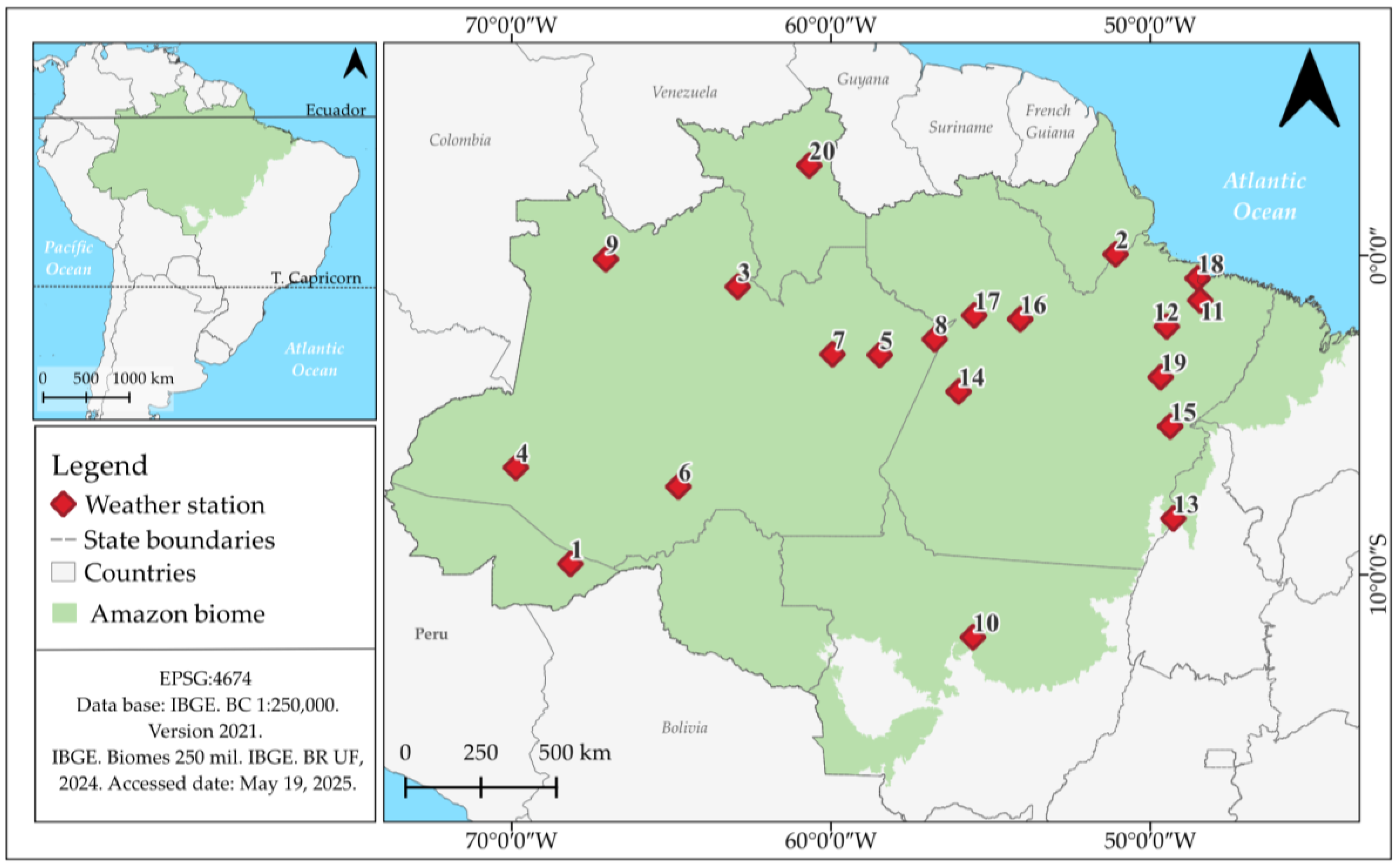
Figure 2.
Organizational structure of the artificial neural network developed for MLP.
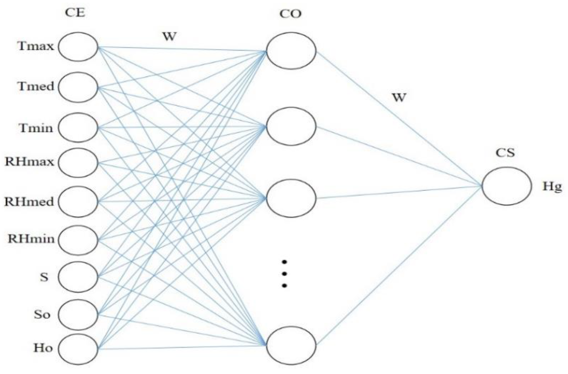
Figure 3.
Schematic representation of the Support Vector Machine (SVM).
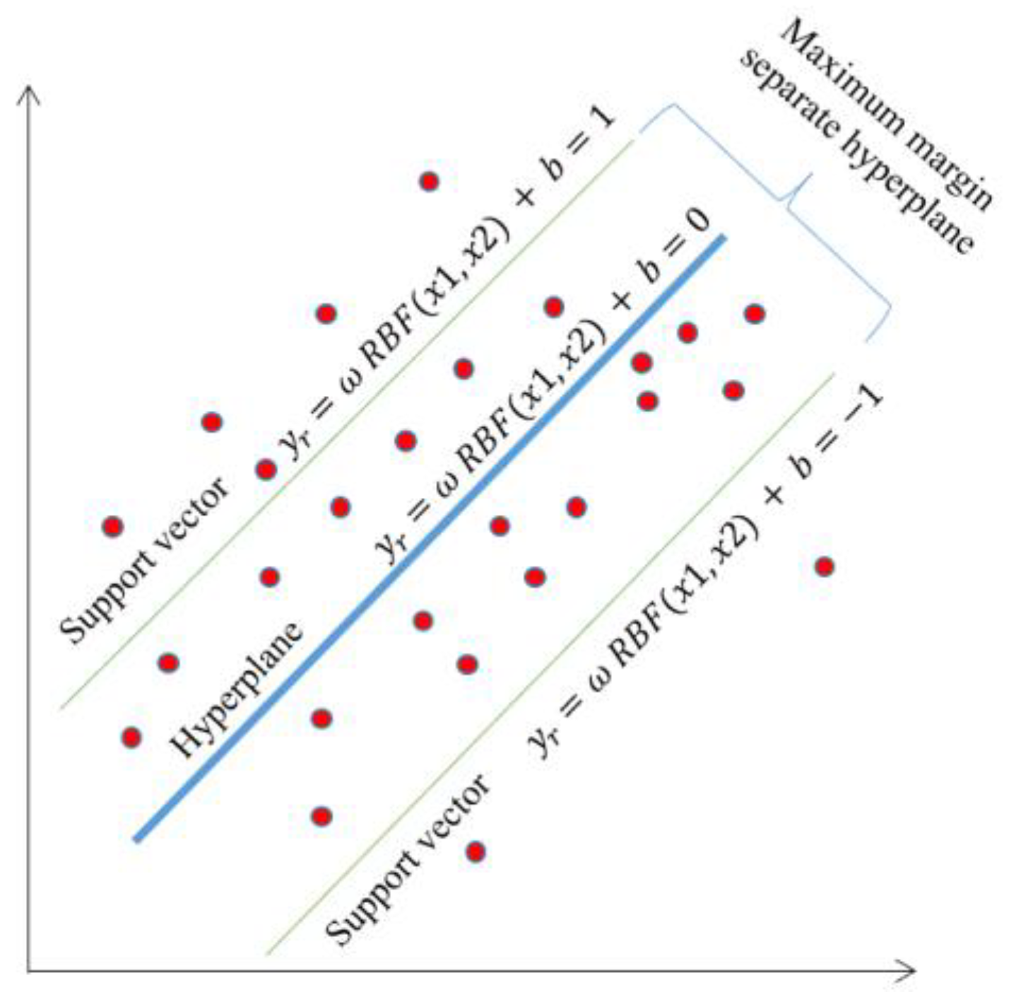
Figure 4.
Pearson correlation (r) between meteorological variables obtained by the 20 weather stations (AWSs and CWSs) located in the Brazilian Amazon biome.
Figure 4.
Pearson correlation (r) between meteorological variables obtained by the 20 weather stations (AWSs and CWSs) located in the Brazilian Amazon biome.
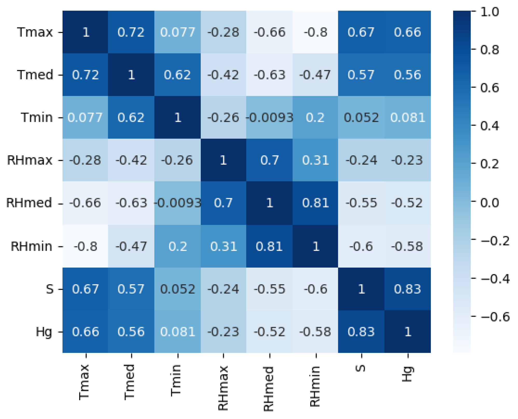
Figure 5.
Boxplot of coefficients of determination (R2), mean relative error (MBE), root mean square error (RMSE) and Willmott coefficient (d), for the MLP in 40 combinations of input variables and the three simplified models, for estimates of daily global radiation at 20 meteorological stations in the Brazilian Amazon biome. (The different colors represent the groupings of the combinations; the hatched area highlights the simplified models).
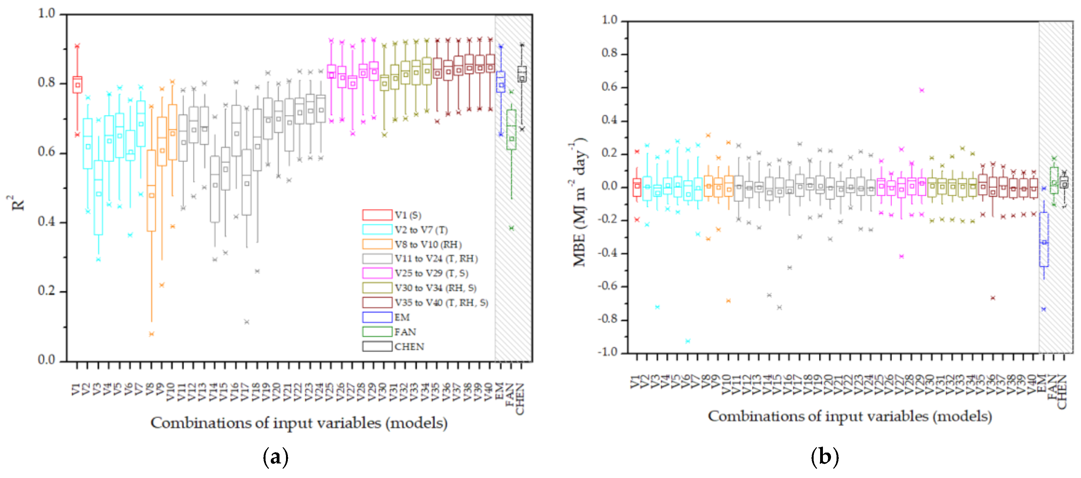
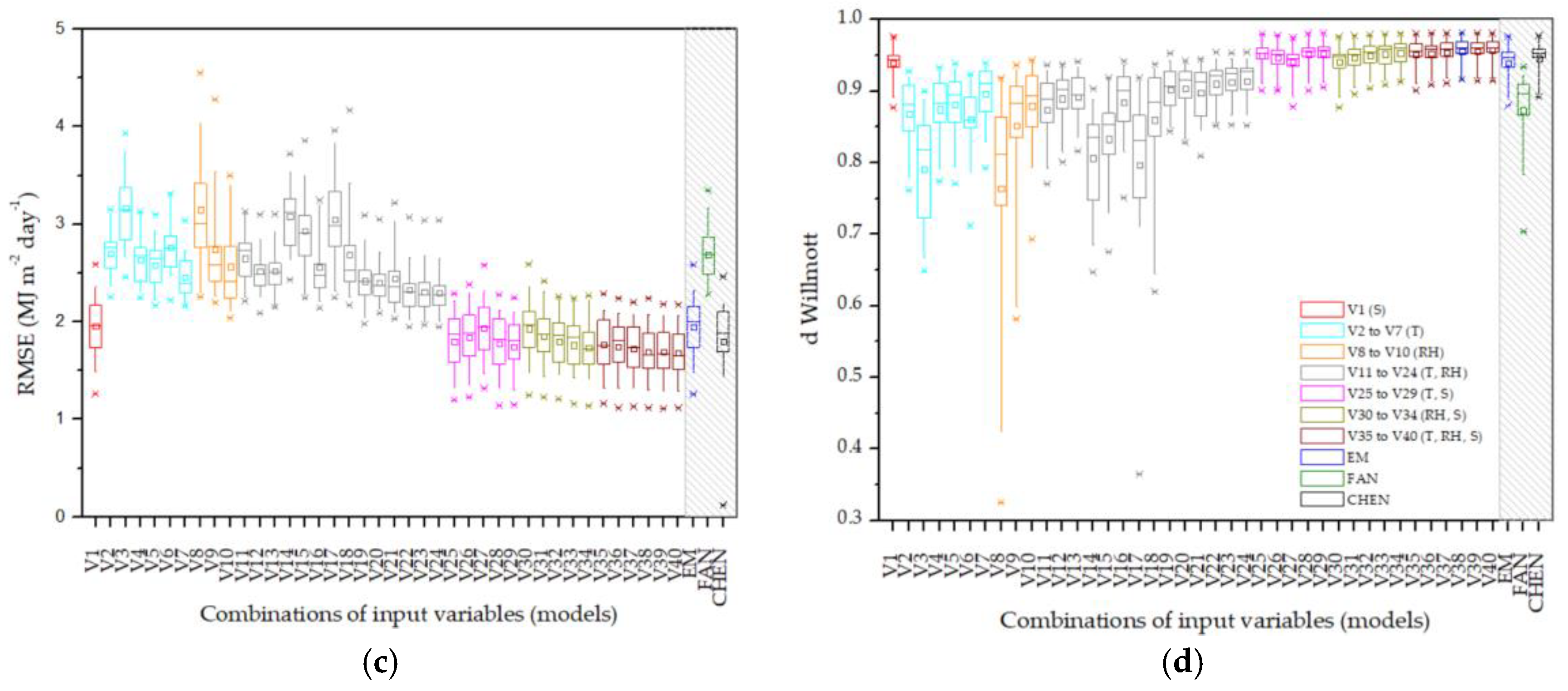
Figure 6.
Boxplot of coefficients of determination (R2), mean relative error (MBE), root mean square error (RMSE) and Willmott coefficient (d), for the SVM in 40 combinations of input variables and the three simplified models, for estimates of daily global radiation at 20 meteorological stations in the Brazilian Amazon biome. (The different colors represent the groupings of the combinations; the hatched area highlights the simplified models).
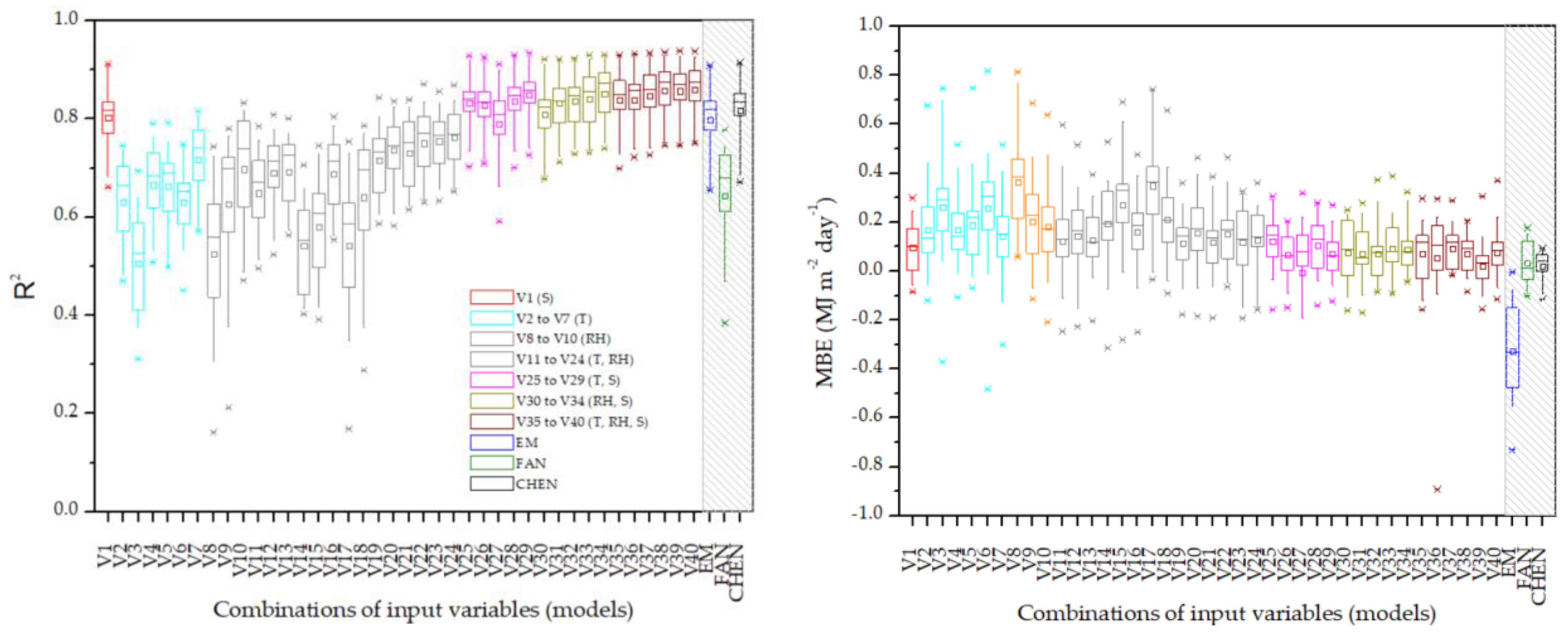
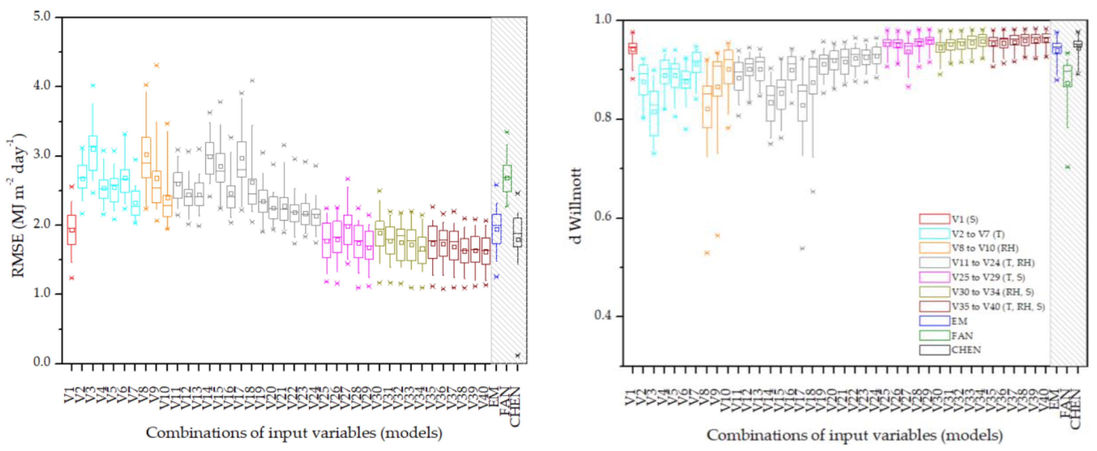
Figure 7.
Dispersion between measured and estimated daily values of global radiation (Hg) by some MLP and SVM techniques (considering only three combinations of input variables V1, V7 and V28), under different sky coverage conditions, at the meteorological stations of Boa Vista, Manaus and Sinop, in the Brazilian Amazon.
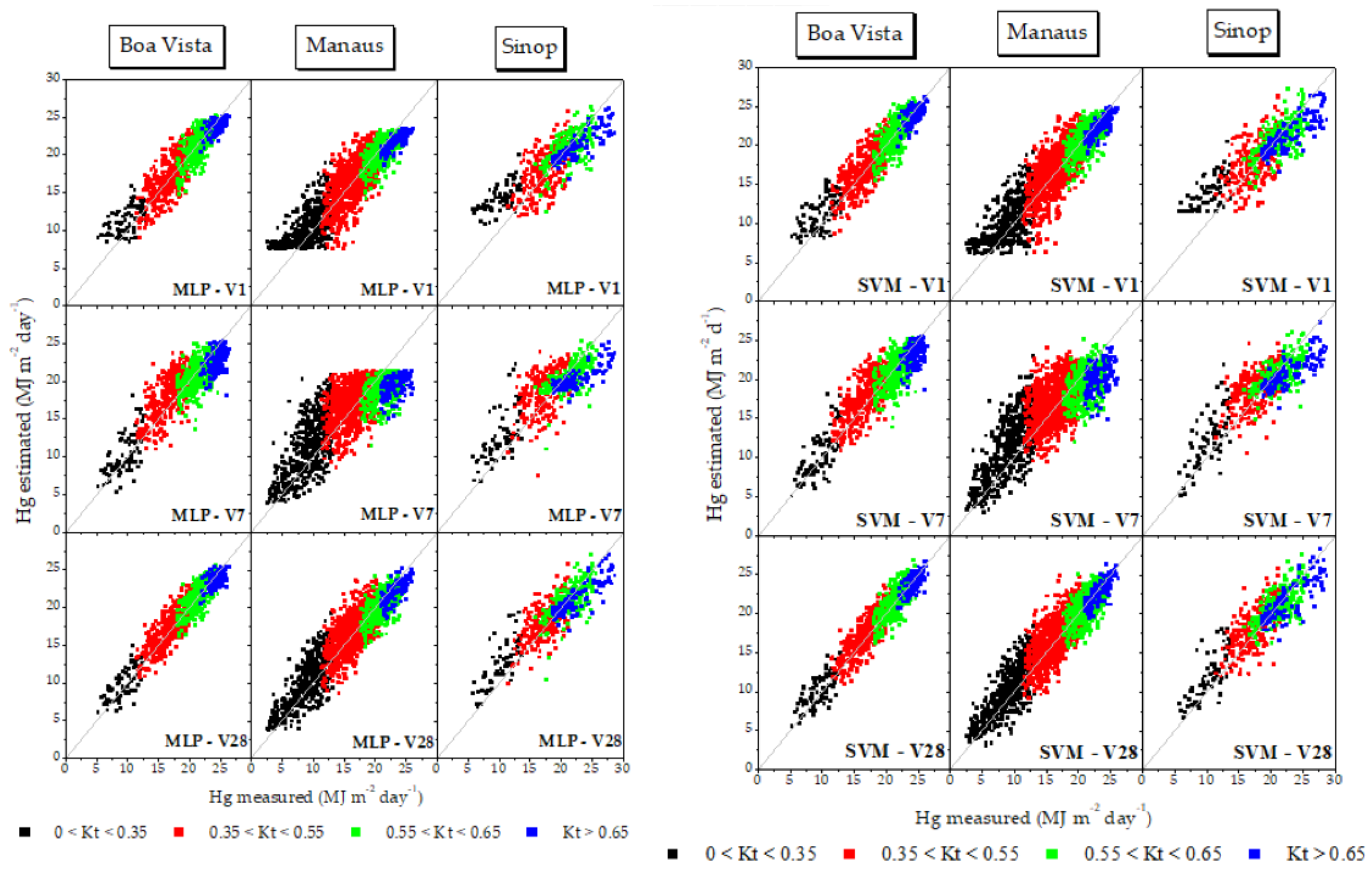
Figure 8.
Dispersion between measured global radiation and global radiation estimated by MLP, SVM and simplified empirical models, for the meteorological stations of Boa Vista, Manaus and Sinop, considering different input variables of the models.
Figure 8.
Dispersion between measured global radiation and global radiation estimated by MLP, SVM and simplified empirical models, for the meteorological stations of Boa Vista, Manaus and Sinop, considering different input variables of the models.
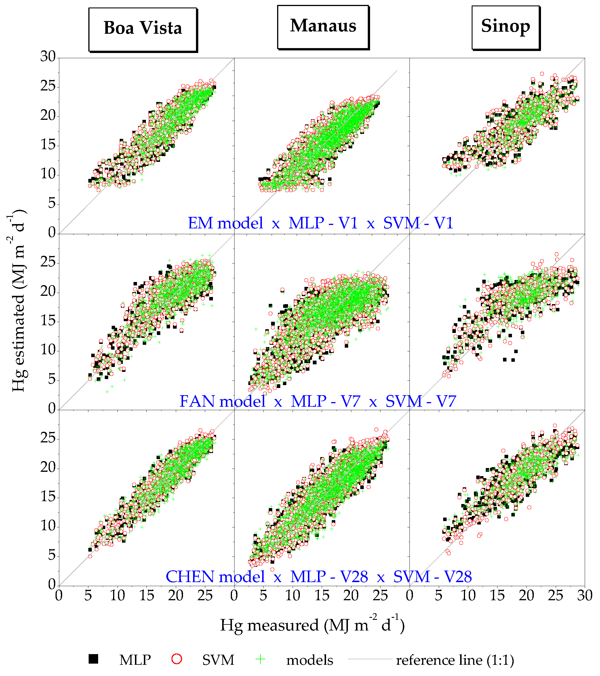
Figure 9.
Frequency of absolute error in the estimation of global radiation using empirical model and ML techniques with insolation as input variable (A), air temperature (B) and hybrid combination (C) as input variable for the meteorological stations of Boa Vista, Manaus and Sinop.
Figure 9.
Frequency of absolute error in the estimation of global radiation using empirical model and ML techniques with insolation as input variable (A), air temperature (B) and hybrid combination (C) as input variable for the meteorological stations of Boa Vista, Manaus and Sinop.
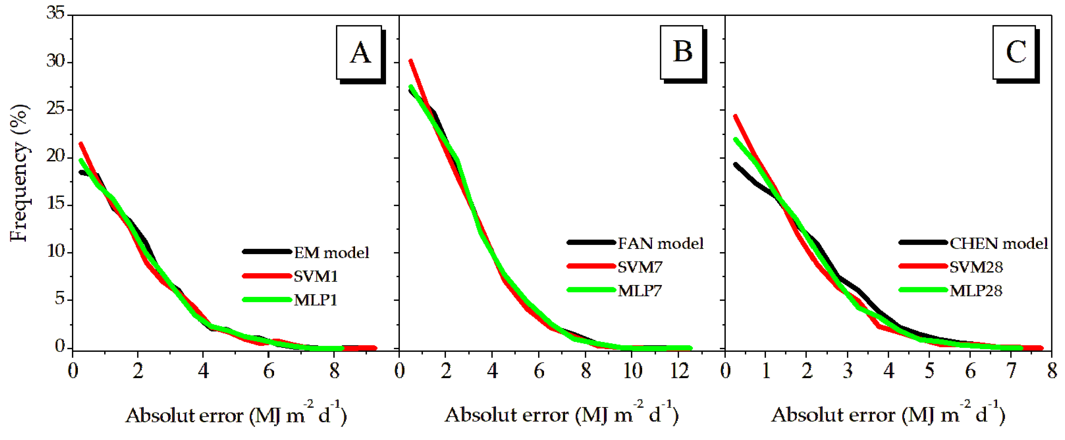

Table 1.
Meteorological stations were installed in the Brazilian Amazon.
| State | City or Station name | KCC* | Lat. | Lon. | Alt. | Operating period |
|---|---|---|---|---|---|---|
| Acre | 1 - Rio Branco | Am | -9.67 | -68.16 | 163 | 2015-2022 |
| Amapá | 2 – Macapá | Am | 0.035 | -51.08 | 16 | 2013-2022 |
| Amazonas | 3 – Barcelos | Af | -0.98 | -62.92 | 29 | 2008-2022 |
| 4 – Eirunepé | Af | -6.65 | -69.87 | 121 | 2012-2022 | |
| 5 – Itacoatiara | Af | -3.12 | -58.47 | 41 | 2008-2022 | |
| 6 – Lábrea | Am | -7.25 | -64.78 | 61 | 2008-2018 | |
| 7 – Manaus | Af | -3.1 | -59.95 | 61 | 2000-2022 | |
| 8 – Parintins | Af | -2.63 | -56.75 | 18 | 2008-2018 | |
| 9 - São Gabriel da Cachoeira | Af | -0.12 | -67.05 | 79 | 2011-2022 | |
| Mato Grosso | 10 – Sinop | Aw | -11.97 | -55.55 | 366 | 2006-2017 |
| Pará | 11 - Belém | Af | -1.41 | -48.43 | 21 | 2003-2022 |
| 12 - Cametá | Af | -2.23 | -49.48 | 9 | 2008-2022 | |
| 13 - Conceição do Araguaia | Aw | -8.25 | -49.27 | 175 | 2008-2022 | |
| 14 - Itaituba | Af | -4.27 | -56.00 | 24 | 2008-2022 | |
| 15 - Marabá | Aw | -5.36 | -49.37 | 116 | 2009-2022 | |
| 16 - Monte Alegre | Am | -2.0 | -54.07 | 100 | 2012-2022 | |
| 17 - Óbidos | Am | -1.88 | -55.51 | 89 | 2012-2017 | |
| 18 - Soure | Am | -0.72 | -48.51 | 12 | 2008-2017 | |
| 19 - Tucuruí | Am | -3.82 | -49.67 | 137 | 2008-2017 | |
| Roraima | 20 - Boa Vista | Am | 2.82 | -60.68 | 82 | 2010-2022 |
Latitude (Lat.); Longitude (Lon.); Altitude (Alt.); KCC: Koppen climate classification, according to Alvares et al. [28].
Table 2.
Different combinations of input variables for Hg estimates using MLP and SVM techniques in the Brazilian Amazon biome.
Table 2.
Different combinations of input variables for Hg estimates using MLP and SVM techniques in the Brazilian Amazon biome.
| Nº | Meteorological variables | Nº | Meteorological variables |
| V1 | S, So, Ho | ||
| V2 | Tmax, So, Ho | V5 | Tmax, Tmin, So, Ho |
| V3 | Tmean, So, Ho | V6 | Tmean, Tmin, So, Ho |
| V4 | Tmax, Tmean, So, Ho | V7 | Tmax, Tmean, Tmin, So, Ho |
| V8 | RHmean, So, Ho | V10 | RHmax, RHmean, RHmin, So, Ho |
| V9 | RHmin, So, Ho | ||
| V11 | Tmax, RHmax, So, Ho | V18 | Tmin, RHmin, So, Ho |
| V12 | Tmax, RHmean, So, Ho | V19 | Tmax, Tmin, RHmax, RHmin, So, Ho |
| V13 | Tmax, RHmin, So, Ho | V20 | Tmax, Tmean, Tmin, RHmean, So, Ho |
| V14 | Tmean, RHmean, So, Ho | V21 | RHmax, RHmean, RHmin, Tmean, So, Ho |
| V15 | Tmean, RHmean, So, Ho | V22 | RHmax, RHmean, RHmin, Tmax, Tmin, So, Ho |
| V16 | Tmean, RHmin, So, Ho | V23 | Tmax, Tmean, Tmin, RHmax, RHmin, So, Ho |
| V17 | Tmin, RHmean, So, Ho | V24 | RHmax, RHmean, RHmin, Tmax, Tmean, Tmin, So, Ho |
| V25 | Tmax, S, So, Ho | V28 | Tmax, Tmin, S, So, Ho |
| V26 | Tmean, S, So, Ho | V29 | Tmax, Tmean, Tmin, S, So, Ho |
| V27 | Tmin, S, So, Ho | ||
| V30 | RHmax, S, So, Ho | V33 | RHmax, RHmin, S, So, Ho |
| V31 | RHmean, S, So, Ho | V34 | RHmax, RHmean, RHmin, S, So, Ho |
| V32 | RHmin, S, So, Ho | ||
| V35 | Tmax, Tmin, Rhmax, S, So, Ho | V38 | RHmax, RHmean, RHmin, Tmax, Tmin, S, So, Ho |
| V36 | Tmax, Tmin, Rhmin, S, So, Ho | V39 | RHmax, RHmin, Tmax, Tmean, Tmin, S, So, Ho |
| V37 | RHmax, RHmin, Tmax, Tmin, So, Ho | V40 | RHmax, RHmean, RHmin, Tmax, Tmean, Tmin, S, So, Ho |
Table 3.
Annual daily averages of meteorological variables (except rainfall) and empirical variables for the 20 meteorological stations evaluated in the Amazon biome.
Table 3.
Annual daily averages of meteorological variables (except rainfall) and empirical variables for the 20 meteorological stations evaluated in the Amazon biome.
| Station | Hg | Ho | S | Tmax | Tmean | Tmin | RHmax | RHmean | RHmin | Rainfall |
| 1 | 17.17±4.80 | 36.23±3.40 | 5.58±3.11 | 31.29±2.84 | 25.60±2.04 | 21.68±1.96 | 91.75±9.71 | 78.42±12.52 | 57.89±15.46 | 2954±139 |
| 2 | 19.86±5.28 | 36.12±1.35 | 6.95±3.23 | 31.76±1.65 | 27.54±1.22 | 23.97±0.73 | 92.67±2.44 | 76.56±1.22 | 55.95±9.10 | 2100±145 |
| 3 | 17.17±5.23 | 35.99±1.34 | 4.77±3.12 | 32.02±2.29 | 26.34±1.23 | 22.76±1.18 | 96.16±2.42 | 83.88±6.11 | 58.88±10.01 | 2443±72 |
| 4 | 15.64±4.25 | 36.36±2.55 | 3.94±2.70 | 31.55±2.27 | 25.92±1.48 | 22.24±1.39 | 86.59±14.76 | 70.16±14.29 | 45.52±16.55 | 1952±75 |
| 5 | 16.12±5.09 | 36.05±1.98 | 5.78±3.33 | 31.52±2.24 | 27.24±1.44 | 24.01±0.98 | 92.72±2.69 | 79.57±6.57 | 59.88±10.56 | 2339±104 |
| 6 | 17.15±3.84 | 35.76±2.95 | 5.24±3.30 | 32.75±2.10 | 26.70±1.30 | 22.57±1.51 | 94.28±1.43 | 78.86±5.96 | 51.90±10.34 | 2230±103 |
| 7 | 16.34±5.04 | 35.91±2.03 | 5.52±3.23 | 32.30±2.21 | 27.74±1.64 | 24.32±1.22 | 91.58±6.38 | 75.86±9.16 | 54.41±11.12 | 2206±99 |
| 8 | 17.52±5.41 | 35.88±1.84 | 6.17±3.41 | 31.29±2.07 | 27.15±1.43 | 24.24±1.09 | 92.66±3.67 | 81.09±6.72 | 62.05±9.19 | 2343±110 |
| 9 | 15.22±4.76 | 36.17±1.30 | 4.73±2.81 | 31.30±2.23 | 26.41±1.45 | 23.14±1.19 | 93.13±5.30 | 81.46±7.99 | 59.18±10.41 | 2867±46 |
| 10 | 19.13±4.19 | 35.95±3.96 | 6.03±3.04 | 32.35±2.81 | 25.41±1.63 | 20.16±2.11 | 91.69±8.05 | 72.04±15.78 | 44.38±16.82 | 1952±132 |
| 11 | 15.09±3.59 | 36.04±1.55 | 6.48±2.75 | 32.67±1.35 | 27.27±1.09 | 23.56±0.65 | 93.22±2.37 | 78.49±5.75 | 54.95±7.22 | 3205±129 |
| 12 | 20.16±3.78 | 35.91±1.79 | 7.57±2.59 | 32.47±1.21 | 27.75±1.13 | 24.23±1.02 | 88.92±4.04 | 74.36±6.15 | 53.30±6.81 | 2230±137 |
| 13 | 18.64±4.46 | 35.79±3.26 | 6.96±3.26 | 33.54±2.75 | 26.83±1.69 | 21.60±2.12 | 90.66±6.24 | 70.50±12.26 | 43.56±15.08 | 1686±104 |
| 14 | 18.75±4.71 | 36.03±2.25 | 6.24±3.18 | 32.67±2.17 | 27.58±1.46 | 23.85±0.96 | 86.22±10.94 | 74.87±7.16 | 60.38±12.95 | 2069±95 |
| 15 | 18.25±3.87 | 35.82±2.57 | 6.36±3.10 | 32.26±1.95 | 26.59±1.14 | 22.40±1.37 | 93.31±2.82 | 76.53±7.75 | 50.78±11.48 | 1885±123 |
| 16 | 20.61±4.19 | 36.13±1.71 | 7.53±2.79 | 31.66±1.69 | 27.54±1.29 | 23.97±1.05 | 87.92±5.38 | 75.30±6.98 | 55.21±8.88 | 1661±104 |
| 17 | 16.64±4.52 | 36.21±2.31 | 6.70±3.21 | 33.08±2.45 | 26.84±1.46 | 22.74±0.78 | 92.77±3.72 | 78.22±8.71 | 52.84±11.51 | 2572±107 |
| 18 | 19.82±4.30 | 35.96±1.38 | 6.89±3.55 | 30.94±0.95 | 27.71±1.04 | 25.34±1.51 | 86.30±6.78 | 76.98±6.03 | 64.05±5.21 | 2093±74 |
| 19 | 16.95±3.48 | 36.06±1.99 | 6.22±2.81 | 31.43±1.68 | 26.73±1.15 | 23.36±0.94 | 94.25±4.29 | 78.42±7.70 | 56.01±9.19 | 2400±157 |
| 20 | 19.35±4.35 | 35.99±1.77 | 6.49±2.87 | 33.51±2.22 | 27.83±1.56 | 23.70±1.07 | 86.69±7.71 | 68.54±10.17 | 45.03±10.41 | 1616±100 |
Global radiation (Hg - MJ m-2 day-1), extraterrestrial radiation (Ho - MJ m-2 day-1), insolation (S - hours), maximum, mean and minimum temperature (Tmax, Tmean, Tmin - °C), maximum, mean and minimum relative humidity (RHmax, RHmean, RHmin - %) and rainfall (mm year-1).
Table 4.
Descriptive analyses of the mean and standard deviation of the residuals for the three weather stations (Boa Vista, Manaus and Sinop), with different input variables in the estimation models.
Table 4.
Descriptive analyses of the mean and standard deviation of the residuals for the three weather stations (Boa Vista, Manaus and Sinop), with different input variables in the estimation models.
| Input variable | Weather station | Estimation model | ||
| EM model | SVM - V1 | MLP - V1 | ||
| Insolation | Boa Vista | - 0.054 ± 1.771 | -0.139 ± 1.664 | -0.051 ± 1.712 |
| Manaus | -0.079 ± 2.253 | -0.245 ± 2.246 | -0.122 ± 2.254 | |
| Sinop | -0.079 ± 2.253 | -0.245 ± 2.246 | -0.122 ± 2.254 | |
| FAN model | SVM - V7 | MLP - V7 | ||
| Air temperature | Boa Vista | -0.070 ± 2.281 | -0.238 ± 2.216 | -0.071 ± 2.380 |
| Manaus | -0.134 ± 3.170 | -0.122 ± 3.080 | -0.001 ± 3.112 | |
| Sinop | -0.323 ± 5.464 | -0.089 ± 2.767 | -0.048 ± 3.018 | |
| CHEN model | SVM - V28 | MLP - V28 | ||
| Hybrid combination | Boa Vista | -0.039 ± 1.720 | -0.119 ± 1.412 | -0.053 ± 1.440 |
| Manaus | -0.083 ± 2.186 | -0.289 ± 2.008 | -0.095 ± 2.046 | |
| Sinop | -0.549 ± 5.655 | 0.038 ± 2.097 | -0.076 ± 2.268 | |
Table 5.
Model Selection Criteria for the three weather stations (Boa Vista, Manaus and Sinop), with the input variables insolation (S), air temperature (Tair) and hybrid combination (S x Tair).
Table 5.
Model Selection Criteria for the three weather stations (Boa Vista, Manaus and Sinop), with the input variables insolation (S), air temperature (Tair) and hybrid combination (S x Tair).
| Station | Criteria | Models | Best model | Model ranking | |||
| Insolação | EM model | SVM 1 | MLP 1 | ||||
| Boa Vista | LL | -1435.480 | -1378.457 | -1402.883 | SVM 1 |
SVM 1 – 1º MLP 1 – 2º EM model – 3º |
|
| AIC | 2876.959 | 2764.914 | 2813.766 | SVM 1 | |||
| BIC | 2891.569 | 2784.394 | 2833.246 | SVM 1 | |||
| BICc | 2884.699 | 2777.524 | 2826.376 | SVM 1 | |||
| WAICa | 2878.959 | 2766.914 | 2815.766 | SVM 1 | |||
| GVC | 3038.945 | 2705.242 | 2845.960 | SVM1 | |||
| Manaus | LL | -3345.215 | -3349.631 | -3347.904 | EM model | EM model – 1º SVM 1 – 2º MLP 1 – 3º |
|
| AIC | 6696.430 | 6707.262 | 6703.808 | EM model | |||
| BIC | 6713.129 | 6729.527 | 6726.073 | EM model | |||
| BICc | 6705.563 | 6721.960 | 6718.507 | EM model | |||
| WAICa | 6698.430 | 6709.262 | 6705.808 | EM model | |||
| GVC | 9840.502 | 9896.006 | 9878.173 | EM model | |||
| Sinop | LL | -1651.183 | -1157.826 | -1164.173 | SVM 1 | SVM 1 – 1º MLP 1 – 2º Modelo 10 – 3º |
|
| AIC | 3308.366 | 2323.653 | 2336.346 | SVM 1 | |||
| BIC | 3321.670 | 2341.391 | 2354.084 | SVM 1 | |||
| BICc | 3315.235 | 2334.957 | 2347.650 | SVM 1 | |||
| WAICa | 3310.366 | 2325.653 | 2338.346 | SVM 1 | |||
| GVC | 20058.800 | 4129.290 | 4214.117 | SVM 1 | |||
| Air temperature | FAN model | SVM 7 | MLP 7 | ||||
| Boa Vista | LL | -1679.145 | -1656.547 | -1719.998 | SVM 7 | SVM 7 – 1º FAN model – 2º MLP 7 – 3º |
|
| AIC | 3368.290 | 3325.094 | 3451.997 | SVM 7 | |||
| BIC | 3392.640 | 3354.314 | 3481.217 | SVM 7 | |||
| BICc | 3385.770 | 3347.444 | 3474.347 | SVM 7 | |||
| WAICa | 3370.290 | 3327.094 | 3453.997 | SVM 7 | |||
| GVC | 5061.517 | 4839.849 | 5521.364 | SVM 7 | |||
| Manaus | LL | -4005.870 | -3950.230 | -3968.264 | SVM 7 | SVM 7 - 1º MLP 7 – 2º FAN model – 3º |
|
| AIC | 8021.740 | 7912.461 | 7948.527 | SVM 7 | |||
| BIC | 8049.572 | 7945.859 | 7981.925 | SVM 7 | |||
| BICc | 8042.006 | 7938.292 | 7974.359 | SVM 7 | |||
| WAICa | 8023.740 | 7914.461 | 7950.527 | SVM 7 | |||
| GVC | 19540.50 | 18465.86 | 18813.70 | SVM 7 | |||
| Sinop | LL | -1631.320 | -1206.492 | -1260.310 | SVM 7 | SVM 7 - 1º MLP 7 – 2º FAN model – 3º |
|
| AIC | 3272.639 | 2424.984 | 2532.620 | SVM 7 | |||
| BIC | 3294.812 | 2451.591 | 2559.228 | SVM 7 | |||
| BICc | 3288.378 | 2445.156 | 2552.793 | SVM 7 | |||
| WAICa | 3274.639 | 2426.984 | 2534.620 | SVM 7 | |||
| GVC | 18942.280 | 4859.383 | 5775.792 | SVM 7 | |||
| Hybrid combination (S x Tair) |
CHEN model | SVM 28 | MLP 28 | ||||
| Boa Vista | LL | -1407.025 | -1220.253 | -1236.760 | SVM 28 | SVM 28 – 1º MLP 28 – 2º CHEN model – 3º |
|
| AIC | 2822.051 | 2452.507 | 2485.520 | SVM 28 | |||
| BIC | 2841.531 | 2481.727 | 2514.740 | SVM 28 | |||
| BICc | 2834.661 | 2474.857 | 2507.870 | SVM 28 | |||
| WAICa | 2824.051 | 2454.507 | 2487.520 | SVM 28 | |||
| GVC | 2870.375 | 1955.652 | 2023.937 | SVM 28 | |||
| Manaus | LL | -3286.880 | -3141.678 | -3160.244 | SVM 28 | SVM 28 - 1º MLP 28 – 2º CHEN model – 3º |
|
| AIC | 6581.760 | 6295.356 | 6332.488 | SVM 28 | |||
| BIC | 6604.025 | 6328.754 | 6365.886 | SVM 28 | |||
| BICc | 6596.459 | 6321.187 | 6358.319 | SVM 28 | |||
| WAICa | 6583.760 | 6297.356 | 6334.488 | SVM 28 | |||
| GVC | 9273.421 | 7996.097 | 8150.956 | SVM 28 | |||
| Sinop | LL | -1654.476 | -1033.619 | -1082.725 | SVM 28 | SVM 28- 1º MLP 28 – 2º CHEN model – 3º |
|
| AIC | 3316.953 | 2079.238 | 2177.449 | SVM 28 | |||
| BIC | 3334.691 | 2105.845 | 2204.057 | SVM 28 | |||
| BICc | 3328.256 | 2099.410 | 2197.622 | SVM 28 | |||
| WAICa | 3318.953 | 2081.238 | 2179.449 | SVM 28 | |||
| GVC | 20337.850 | 2789.800 | 3265.582 | SVM 28 | |||
Table 6.
Synthesis of models with the addition of sunlight, temperature and hybrids, for the three weather stations (Boa Vista, Manaus and Sinop).
Table 6.
Synthesis of models with the addition of sunlight, temperature and hybrids, for the three weather stations (Boa Vista, Manaus and Sinop).
| Stations | Selected models/Ranking | 1º | 2º | 3º |
| Boa Vista | Insolation | SVM 1 | MLP 1 | EM model |
| Air temperature | SVM 7 | FAN model | MLP 7 | |
| Hybrid combination | SVM 28 | MLP 28 | CHEN model | |
| Prevailing model | SVM | MLP | Model | |
| Manaus | Insolation | EM model | SVM 1 | MLP 1 |
| Air temperature | SVM 7 | MLP 7 | FAN model | |
| Hybrid combination | SVM 28 | MLP 28 | CHEN model | |
| Prevailing model | SVM | MLP | Model | |
| Sinop | Insolation | SVM 1 | MLP 1 | EM model |
| Air temperature | SVM 7 | MLP 7 | FAN model | |
| Hybrid combination | SVM 28 | MLP 28 | CHEN model | |
| Prevailing model | SVM | MLP | Model |
Table 7.
Selection criteria applied to the best first-place global radiation models for the three weather stations (Boa Vista, Manaus and Sinop).
Table 7.
Selection criteria applied to the best first-place global radiation models for the three weather stations (Boa Vista, Manaus and Sinop).
| Stations | Criteria | SVM 1 | SVM 7 | SVM 28 | Best Model | Ranking models |
| Boa Vista | LL | -1378.457 | -1656.547 | -1220.253 | SVM 28 | SVM 28 – 1º SVM 1 – 2º SVM 7 – 3º |
| AIC | 2764.914 | 3325.094 | 2452.507 | SVM 28 | ||
| BIC | 2784.394 | 3354.314 | 2481.727 | SVM 28 | ||
| BICc | 2777.524 | 3347.444 | 2474.857 | SVM 28 | ||
| WAICa | 2766.914 | 3327.094 | 2454.507 | SVM 28 | ||
| GVC | 2705.242 | 4839.849 | 1955.652 | SVM 28 | ||
| Manaus | LL | -3349.631 | -3950.230 | -3141.678 | SVM 28 | SVM 28 – 1º SVM 1 – 2º SVM 7 – 3º |
| AIC | 6707.262 | 7912.461 | 6295.356 | SVM 28 | ||
| BIC | 6729.527 | 7945.859 | 6328.754 | SVM 28 | ||
| BICc | 6721.960 | 7938.292 | 6321.187 | SVM 28 | ||
| WAICa | 6709.262 | 7914.461 | 6297.356 | SVM 28 | ||
| GVC | 9896.006 | 18465.86 | 7996.097 | SVM 28 | ||
| Sinop | LL | -1157.826 | -1206.492 | -1033.619 | SVM 28 | SVM 28 – 1º SVM 1 – 2º SVM 7 – 3º |
| AIC | 2323.653 | 2424.984 | 2079.238 | SVM 28 | ||
| BIC | 2341.391 | 2451.591 | 2105.845 | SVM 28 | ||
| BICc | 2334.957 | 2445.156 | 2099.410 | SVM 28 | ||
| WAICa | 2325.653 | 2426.984 | 2081.238 | SVM 28 | ||
| GVC | 4129.290 | 4859.383 | 2789.800 | SVM 28 |
Table 8.
Selection criteria applied to the best second-place global radiation models for the three weather stations (Boa Vista, Manaus and Sinop).
Table 8.
Selection criteria applied to the best second-place global radiation models for the three weather stations (Boa Vista, Manaus and Sinop).
| Stations | Criterias | MLP 1 | MLP 7 | MLP 28 | Best model | Rankin model |
| Boa Vista | LL | -1402.883 | -1719.998 | -1236.760 | MLP 28 | MLP 28 – 1º MLP 1 – 2º MLP 7 – 3º |
| AIC | 2813.766 | 3451.997 | 2485.520 | MLP 28 | ||
| BIC | 2833.246 | 3481.217 | 2514.740 | MLP 28 | ||
| BICc | 2826.376 | 3474.347 | 2507.870 | MLP 28 | ||
| WAICa | 2815.766 | 3453.997 | 2487.520 | MLP 28 | ||
| GVC | 2845.960 | 5521.364 | 2023.937 | MLP 28 | ||
| Manaus | LL | -3347.904 | -3968.264 | -3160.244 | MLP 28 | MLP 28 – 1º MLP 1 – 2º MLP 7 – 3º |
| AIC | 6703.808 | 7948.527 | 6332.488 | MLP 28 | ||
| BIC | 6726.073 | 7981.925 | 6365.886 | MLP 28 | ||
| BICc | 6718.507 | 7974.359 | 6358.319 | MLP 28 | ||
| WAICa | 6705.808 | 7950.527 | 6334.488 | MLP 28 | ||
| GVC | 9878.173 | 18813.70 | 8150.956 | MLP 28 | ||
| Sinop | LL | -1164.173 | -1260.310 | -1082.725 | MLP 28 | MLP 28 – 1º MLP 1 – 2º MLP 7 – 3º |
| AIC | 2336.346 | 2532.620 | 2177.449 | MLP 28 | ||
| BIC | 2354.084 | 2559.228 | 2204.057 | MLP 28 | ||
| BICc | 2347.650 | 2552.793 | 2197.622 | MLP 28 | ||
| WAICa | 2338.346 | 2534.620 | 2179.449 | MLP 28 | ||
| GVC | 4214.117 | 5775.792 | 3265.582 | MLP 28 |
Table 9.
Selection criteria applied to the best third-place global radiation models for the three weather stations (Boa Vista, Manaus and Sinop).
Table 9.
Selection criteria applied to the best third-place global radiation models for the three weather stations (Boa Vista, Manaus and Sinop).
| Station | Criteria | EM model | FAN model | CHEN model | Best model | Ranking model |
| Boa Vista | LL | -1435.480 | -1679.145 | -1407.025 | CHEN model | CHEN model – 1º EM model – 2º FAN model – 3º |
| AIC | 2876.959 | 3368.290 | 2822.051 | CHEN model | ||
| BIC | 2891.569 | 3392.640 | 2841.531 | CHEN model | ||
| BICc | 2884.699 | 3385.770 | 2834.661 | CHEN model | ||
| WAICa | 2878.959 | 3370.290 | 2824.051 | CHEN model | ||
| GVC | 3038.945 | 5061.517 | 2870.375 | CHEN model | ||
| Manaus | LL | -3345.215 | -4005.870 | -3286.880 | CHEN model | CHEN model – 1º EM model – 2º FAN model – 3º |
| AIC | 6696.430 | 8021.740 | 6581.760 | CHEN model | ||
| BIC | 6713.129 | 8049.572 | 6604.025 | CHEN model | ||
| BICc | 6705.563 | 8042.006 | 6596.459 | CHEN model | ||
| WAICa | 6698.430 | 8023.740 | 6583.760 | CHEN model | ||
| GVC | 9840.502 | 19540.50 | 9273.421 | CHEN model | ||
| Sinop | LL | -1651.183 | -1631.320 | -1654.476 | FAN model | FAN model – 1º EM model – 2º CHEN model– 3º |
| AIC | 3308.366 | 3272.639 | 3316.953 | FAN model | ||
| BIC | 3321.670 | 3294.812 | 3334.691 | FAN model | ||
| BICc | 3315.235 | 3288.378 | 3328.256 | CHEN model | ||
| WAICa | 3310.366 | 3274.639 | 3318.953 | CHEN model | ||
| GVC | 20058.800 | 18942.280 | 20337.850 | CHEN model |
Table 10.
Description of model indicates global selection of models, in order of placement.
| Best Model Settings | Order of Models |
| 1º: Hybrid models | SVM -V28 – 1º; MLP -V28 – 2º; CHEN model – 3º |
| 2º: Models based on insolation | SVM - V1– 1º; MLP - V1 – 2º; EM model – 3º |
| 3º: Models based on air temperature | SVM - V7 – 1º; MLP - V7 – 2º; FAN model – 3º |
Disclaimer/Publisher’s Note: The statements, opinions and data contained in all publications are solely those of the individual author(s) and contributor(s) and not of MDPI and/or the editor(s). MDPI and/or the editor(s) disclaim responsibility for any injury to people or property resulting from any ideas, methods, instructions or products referred to in the content. |
© 2025 by the authors. Licensee MDPI, Basel, Switzerland. This article is an open access article distributed under the terms and conditions of the Creative Commons Attribution (CC BY) license (http://creativecommons.org/licenses/by/4.0/).
Copyright: This open access article is published under a Creative Commons CC BY 4.0 license, which permit the free download, distribution, and reuse, provided that the author and preprint are cited in any reuse.


