
Submitted:
28 May 2025
Posted:
30 May 2025
You are already at the latest version
Abstract
Using the technique of inductive resolution introduced by Hepworth, Patzt and Boyd, we prove that the homology of Rook-Brauer Algebra, interpreted as appropriate Tor-group, is isomorphic to that of symmetric group for all degrees under the assumption that $\epsilon$ in $R$ is invertible; furthermore, we also prove the homology of the Motzkin algebras vanishes in positive degrees under the same assumption. These results thereby establish homological stability of both algebras.
Keywords:
diagram algebras
; homology
; homological stability
; rook-brauer algebras
; motzkin algebras
1. Introduction
The Rook-Brauer Algebras and Motzkin Algebras are part of the family of diagram algebras that includes the Partition Algebra, Rook Algebra, Temperley-Lieb Algebra, Brauer Algebra, and many more. In recent years, homology of these algebras has been studied extensively by various authors (see [1] for partition algebras, [2] for Temperley-Lieb Algebras, [3] for Brauer Algebras, [4] for Rook and Rook-Brauer Algebras with restriction on parameters, see [6] for Tanabe algebras, uniform block permutation algebras and totally propagating partition algebras).
The results of most diagram algebras mentioned above are parameters-dependent i.e certain conditions, most notably the invertibility of the parameter, must be imposed to ensure the validity of these results. The Rook-Brauer algebra has two defining parameters, and (which will be recalled later), and in [4], Guy Boyde attempted to use the concept of idempotents to demonstrate that the homology of Rook-Brauer algebras is isomorphic to that of symmetric groups in all degrees, provided that is invertible. However, as noted by Andrew Fisher and Daniel Graves in their paper (see Remark 7.1.1 [7]), the argument presented was found to be incorrect. Fisher and Graves, by additionally assuming the invertibility of , were able to refine and correct the approach, ultimately proving that the homology of the Rook-Brauer algebras is indeed isomorphic to that of the symmetric groups in all degrees (see Theorem 7.1.5 [7]). Furthermore, under the same assumption on and , they also proved that the homology of the Motzkin algebras vanishes in positive degrees (see Theorem 7.1.6 [7]).
In this paper, we employ the technique of inductive resolution pioneered by Boyd, Hepworth and Patzt in [1] to prove the same results as those of Fisher and Graves for Rook-Brauer and Motzkin algebras while only requiring the invertibility of ϵ. More specifically, under the assumption that is invertible and for any where R is a unital commutative ring, we prove that the homology of the Rook-Brauer algebra is isomorphic to that of the symmetric group for all degrees and the homology of the Motzkin Algebras vanishes in positive degrees.
2. Main Result
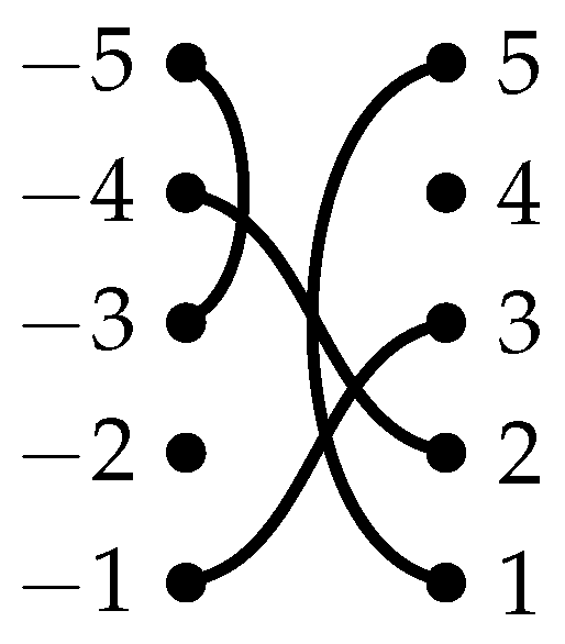
We now introduce the background necessary to discuss our main results. For a unital commutative ring R, the Rook-Brauer Algebras with parameters is a free R-module with basis consisting of partitions of the unions of the sets whose blocks (components) have size where and . Each basis element of may be visualized by a diagram with two vertical columns of n nodes each, with the nodes on the left representing through and the nodes on the right representing 1 through n, with paths connecting certain nodes. Since each block has size at most 2, each basis element is represented by a diagram in which each node is connected to at most one other node and isolated nodes are allowed. Below is an example of a diagram in .
Figure 1.
Visualization of the partition .
Multiplying two diagrams, and , involves placing them side by side and identifying their middle nodes to create a new diagram, . In this process, any loop that appears in the middle is replaced by a factor of , and any contractible component in the middle is replaced by a factor of .
The Motzkin Algebras is the R-subalgebra of with basis given by planar Rook-Brauer diagrams i.e Rook-Brauer diagrams where connections cannot cross.
Diagrams in which every node on the left is connected to a single node on the right are called permutation diagrams, and are in bijection with elements of the symmetric group . This gives us an inclusion and projection of algebras
For each n, and are augmented algebras equipped with the augmented map that sends permutation diagrams to and all other diagrams to . This, in turn, makes R a trivial module of and which we denoted by . By homology of Rook-Brauer algebras and Motzkin algebras , we mean the Tor groups and , respectively.
The inclusion map and projection map also induce the corresponding maps and on homology groups such that is the identity. Hence, homology of is a direct summand of the homology of .
We state our main results:
Theorem 1.
Suppose that ϵ is invertible in R and for any , the inclusion map induces a map in homology
that is an isomorphism for all degrees *.
Under the same hypothesis, the homology of the Motzkin algebra vanishes in positive degrees.
Theorem 2.
Suppose that ϵ is invertible in R and for any ,
Combining these theorems with the homological stability of symmetric groups proved by Nakaoka in [7] in which the stable range is sharp yields the following corollary.
Corollary 1.
Suppose that ϵ is invertible in R and for any , the Rook-Brauer algebras satisify homological stability i.e the inclusion induces a map
that is an isomorphism in degrees , and this stable range is sharp.
Under the same assumption, the Motzkin algebras also satisfies homological stability.
3. Rook-Brauer and Motzkin Algebras
In this section, we recall the definition of the Rook-Brauer and Motzkin algebras, certain diagrams and results that will be used in later sections.
3.1. Rook-Brauer Algebras
Definition 1.
For a unital commutative ring R, the Rook-Brauer algebra with parameters is a free R-module with basis consisting of partitions of the unions of the sets whose blocks (components) have size where and . Each basis element of may be visualized by a diagram α with two vertical columns of n nodes each, with the nodes on the left representing through and the nodes on the right representing 1 through n, with paths connecting certain nodes. Since each block has size at most 2, each basis element is represented by a diagram in which each node is connected to at most one other node and isolated nodes are allowed.
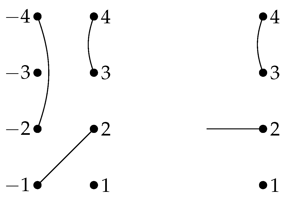
For diagrams and , we define the product in the following way. First we conjoin the diagrams and by identifying each node k on the right of with the node on the left of , thus forming a diagram with 3 columns of n nodes each. We then form a new partition of in which two elements belong to the same block if and only if the corresponding nodes in the left or right column of the conjoined diagram are connected. We define where r is the number of loops and s is the number of contractible components in the middle column (see example below).
Figure 2.
Multiplication in .
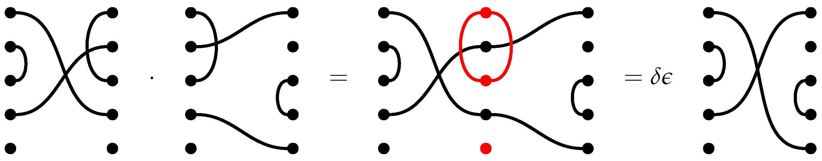
Here, the final diagram is multiplied by a factor of for the red loop and a factor of for the isolated node in the middle.
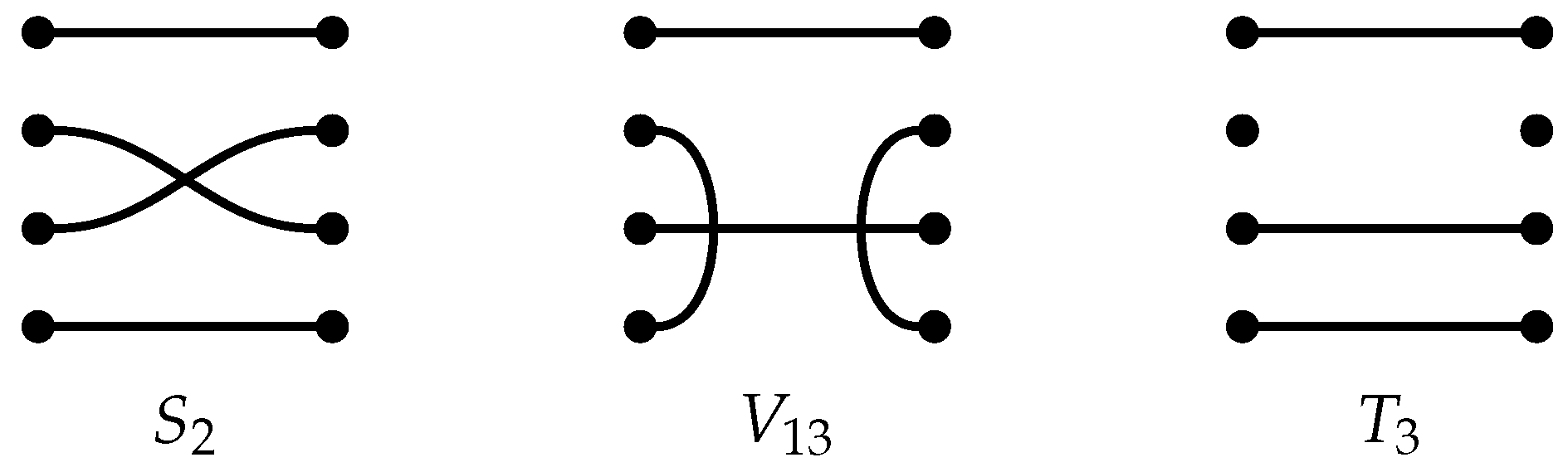
We also point out here three specific types of diagram (see Figure ) that will be used later:
- For , is the permutation diagram corresponding to the partition with blocks of pairs for , together with and . These generate the group ring of the symmetric group, , as a subalgebra of .
- For , is the diagram corresponding to the partition with blocks of pairs for and two blocks consists of and .
- For , is the diagram corresponding to the partition with blocks of pairs for and two singleton blocks and .
Figure 3.
The elements .
Recall that permutation diagrams of are diagrams where each node on the left is connected to a node on the right i.e there are no isolated nodes or same-side connections in these diagram.
Definition 2.
(Trivial module ) For any n, we define the trivial -module to be a single copy of R where permutation diagrams acts as the identity and all other diagrams acts as zero.
Definition 3.
For , we can view as a subalgebra of as follows: given a diagram α in , we can add horizontal connectionsbelowα to form a diagram in . Then, under the action of this subalgebra, can be viewed as a left -module and a right -module, and we obtain the induced left -module .
It turns out that the left -module is a free R-module whose basis are given in terms of special diagrams as described by the following Proposition from [9].
Proposition 1
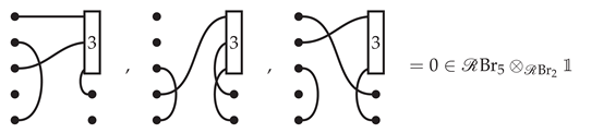
([9], Proposition 3.1). is a free R-module with a basis consisting of diagrams with n nodes on the left, m nodes on the right under a box containing the top nodes subject to these conditions:
- Each node is either connected to the box, to another node, or remains isolated. The box must be connected to exactly nodes.
- Any diagram in which the box is connected to fewer than nodes is identified with 0.
Some (non-)examples of these basis diagrams in are given below.
3.2. Motzkin Algebras
Definition 4.
AMotzkin n-diagramis a planar Rook-Brauer n-diagram i.e diagrams where connections cannot cross. TheMotzkin algebras, , is an R-subalgebra of with basis given by all Motzkin n-diagrams.
Note that, due to the restriction of planarity, the only permutation diagram in is the identity diagram i.e diagram with all horizontal left-to-right connections. Since is a subalgebra of , we also have the trivial-module as in Def. 2.
We recall the definition of link states for a Motzkin diagram below. Although this concept can be defined more generally for Rook–Brauer diagrams, our focus here is solely on the Motzkin diagram.
Definition 5.
By slicing vertically down the middle of a Motzkin n-diagram, we obtain two "half-diagrams" which are calledleft link stateandright link stateof the diagram. Explicitly, a link state consists of a column of n nodes where at each node, we have one of the following situations:
- The node has a hanging edge called adefecti.e an edge whose other end is not attached to anything.
- The node is connected to exactly one other node.
- The node is an isolated node.
Since a Motzkin diagram is a planar diagram, the right and left link state of it is also planar. Below is an example of a Motzkin diagram and its right link state.
Figure 4.
A Motzkin 4-Diagram and Its Right Link State
Definition 6.
Given a right link state of a Motzkin n-diagram, we can remove two defects and replace them with a right-to-right connection joining the two vertices. This operation is called a splice . We can also remove a defect, leaving an isolated vertex. This operation is called a deletion. Note that all splice operations must respect the planarity condition.
4. Inductive Resolution
A key tool in many proofs of the homological stability of groups is Shapiro’s Lemma. However, when dealing with algebras that do not arise as group algebras, Shapiro’s Lemma does not always apply as the algebra A may fail to be flat over its subalgebras (see sect 4 of [3] and sect 1 of [2]). To address this issue, we will use inductive resolution prove an analogue (more general) version of Shapiro’s Lemma for the Rook-Brauer Algebra.
Simply put, the technique of inductive resolution provides a method for proving the vanishing of of a given module by resolving it through modules that already possess this property- hence the term "inductive" resolution. We formally state the principle of inductive resolution as introduced in [1].
Theorem 3
([1], Theorem 3.1). Let A be an algebra over a ring R, and let M be a right A-module. Suppose that N is a left A-module equipped with a resolution with the following two properties:
- vanishes in positive degrees for all .
- is a resolution.
Then vanishes in positive degrees.
For the rest of this section, we will use the technique of inductive resolution to prove Tor of certain modules vanishes for positive degrees.
4.1. Inductive Resolution for Rook-Brauer Algebras
Definition 7.
Suppose that X is a subset of the set . Define to be the left-ideal in that is the R-span of all diagrams in which, among the nodes on the right labeled by elements of X, there is at least one singleton or a right-to-right connection. For , let be denoted by .
Notice that is spanned by all non-permutation diagrams of so . We will use inductive resolution to establish the following theorem, which will play a key role in proving the analogues of Shapiro’s Lemma.
Theorem 4.
Let and suppose is invertible and , then the groups vanish in positive degrees.
The proof of this result will occupy the rest of this section and we follow a similar outline as Section 4 of [1] with some modifications. Below, we prove a short lemma that is necessary for Theorem 2.
Lemma 1.
In particular,
for all .
Let J be a left ideal of that is included in . Then
Proof.
Since , elements of J acts as zero on and this gives □
We will prove Theorem 2 by induction on the cardinality of and to do that, we will resolve in term of these special modules introduced below.
Definition 8.
Let , and let , define three left -submodules of as follows:
- is the span of all diagrams in which x is a singleton.
- is the span of all diagrams in which x is connected to some element of X.
- is the span of all diagrams in which nodes a and b are connected.
We also define the quotients:
We prove some results about these special modules.
Lemma 2.
Let be invertible. The modules , , and behave as follows under tensor product with .
- Let . Then and is a direct summand of .
- Let with . Then .
- Let , then . Furthermore, is a direct summand of .
Proof.
because and in the second case are both non-permutation diagrams and hence, acts as 0 on .
we will show that this map is surjective and splits. To see that the map is surjective, pick any diagram , we then have which shows that the map is surjective.
Since are quotients of and respectively, we show that these modules vanish when tensoring with .
To show , let be a diagram in which means node x is a singleton. This means also has another singleton on the left or right side, say . If is on the left, then and if is on the right, then where in both cases, is the diagram obtained from by connecting x and together while leaving all other connections unchanged. Then, in both cases,
For the second part, we prove that is a direct summand of . Since right-multiplying by takes to itself, this induces the map . This map is surjective because for any diagram , we have ; it also splits because is idempotent with splitting map induced by the inclusion .
To show , let be a diagram, then the node x is connected to some node y of X. Since each node is connected to at most one other node in any Rook-Brauer diagram, this implies that there is either a left-to-left connection or a pair of isolated nodes on the left.
Case 1: If there is a left-to-left connection from to , choose to be the diagram obtained from by removing the connection from x to y. Notice that .
Case 2: If there is a pair of isolated nodes on the left, choose to be the diagram obtained from by removing the connection from x to y, then either connect with x or with y but not both. Notice that .
In both case, is a non-permutation diagram which gives .
Finally, we conclude that by applying the second part above. To see that is a direct summand of , note that right-multiplication by takes into itself so this induces the map
This map also splits because is idempotent with the splitting map induced by the inclusion . □
One can readily verify that decomposes as a direct sum of ’s as follows.
Lemma 3.
For any , there exists a left -modules isomorphism .
Proof.
The isomorphism is given by where, on each summand, is the map induced by the inclusions
To see that is surjective, observe that for any diagram , the node x must be connected to some node . This means lies in the image of the direct summand indexed by , which shows that is indeed surjective.
Note that images of diagrams from different direct summand are distinct because for , diagrams in has node x connected with while diagrams in has node x connected with . Hence, to show that is injective, we can show for each direct summand, is injective. Pick a diagram in the kernel of this map i.e in . This implies lies in which means, two nodes of labeled by elements of must be connected or a node labeled by is isolated.
Since lies in , is not isolated and is connected with x. Hence, must have a right-to-right connection between two nodes labeled by or an isolated node among nodes labeled by . But this implies so this map is injective, hence is also injective. □
We now resolve in terms of and . The proof of the following proposition is almost identical, with small modifications, to the proof of Proposition 4.6 presented in [1].
Proposition 2.
Let , let , and assume . The following sequence, in which all maps are induced by either an inclusion or an identity map, is a resolution of .
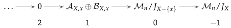 Moreover, applying to the sequence gives a resolution of .
Proof.
Since all maps are induced by either inclusion or identity, all maps are well-defined because , and . The surjectivity of the map is clear so the complex is exact at degree . To see the complex is exact at degree 0, we observe that the kernel of the map is spanned by diagrams in that lies in . For a diagram to be in , there must be a right-to-right connection or an isolated node among nodes labeled by X. For it to also not be in , among nodes labeled by X, it must have exactly one right-to-right connection between x and another node in X or x must be the only isolated node. If has a right-to-right connection between x and another node in X, then is in the image of the inclusion . If x is an isolated node in , then is in the image of the inclusion . Hence, the complex is exact at degree 0. To show exactness at degree 1 i.e the map is injective, note that if and such that , then because and have no basis elements in common. Hence, the complex is exact at degree 1 and it is a resolution of . To prove the second claim, after applying and by Lemmas 2 and 1, the resolution becomes
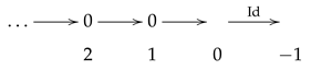 and the claim now follows. □
We use this proposition to prove the vanishing of Tor’s group of , Theorem 4. The proof below follows a similar outline with some modifications to that of the analogous statement for Partition algebras. (see section 4.4 of [1]).
Proof of Theorem 4 For the case when , we have and the result follows immediately. For the case when , we either have or . If , then so that and the result follows. If , then is spanned by which implies and we have a SES

Since is invertible, and are direct summand of and the result now follows. Assume that and . We prove the theorem by using strong induction on cardinality of X. From above, the result is clear when . Assume and the result holds for any subset of smaller cardinality. By Proposition 2 and Theorem 3, it suffices to show that the three modules and all vanish under for . But this is immediate since for because of the induction hypothesis and for because is a direct summand of by Lemma 2, which vanishes under so does as well. By Lemma 3, is a direct summand of ’s for and Lemma 2 implies is also a direct summand of which vanishes under because of the induction hypothesis. This, in turn, implies also vanishes under and so does . □
4.2. Inductive Resolution for Motzkin Algebras
This subsection is similar to the subsection 4.1 above and we will prove the analogue of Theorem 4 for the Motzkin algebras.
By replacing with in Definition 7 and 8, we obtain similar left -submodules of , namely , , and the corresponding quotients , . We also introduce a new left -submodule tailored specifically to the structure of Motzkin algebras.
Notational Remark: For with , define .
Definition 9.
Let with , if P is a partition of into subsets of size at most 2, define to be the right-link state of a Motzkin n-diagram in which all right-to-right connections and isolated nodes are in one-to-one correspondence to pairs and singletons, respectively, in P (labeled by pairs and singletons in P) while all other nodes have defects.
If any of the above connections violate planarity, there is no right link state for that particular P.
For example, if and , then is given below.
Figure 5.
when and .
Definition 10.
Given a right-link state , define a left -submodule spanned by diagrams having right-link state obtained from by a (possibly empty) sequence of splices and deletion (see Def 6). If no right-link state exists for P, define to be the zero module.
Definition 11.
Given with , let P be a partition of as above with and the corresponding right-link state , define the quotient
We prove the analogue of Lemma 2 for .
Lemma 4.
Let and P be a partition of if or if as above with , then . Furthermore, is a direct summand of where with .
Proof.
so as needed.
because no sequence of splices/deletions can remove a right-to-right connection. Similarly, if and i.e an isolated node labeled by , then
because of reason similar to above. Hence, in both cases, and is trivially a direct summand of .
.
.
as above. Therefore, is a direct summand of .
To show , we show . For a diagram , define to be the diagram obtained from by preserving all right-to-right connections of and for the other nodes, make all horizontal left-to-right connections without violating planarity.
Note that where k is a nonnegative integer that depends on the number of right-to-right connections and isolated nodes on the right of . Since any diagram in has a right-to-right connection from node x to node y, it is a non-permutation diagram. Hence,
To prove the second claim, WLOG, assume and let . Note that .
To see that is a direct summand of , observe that if and i.e a right-to-right connection between two nodes labeled by , then
For the last case, assume there is no such that i.e no right-to-right connections or isolated nodes labeled by inside the connection x to y.
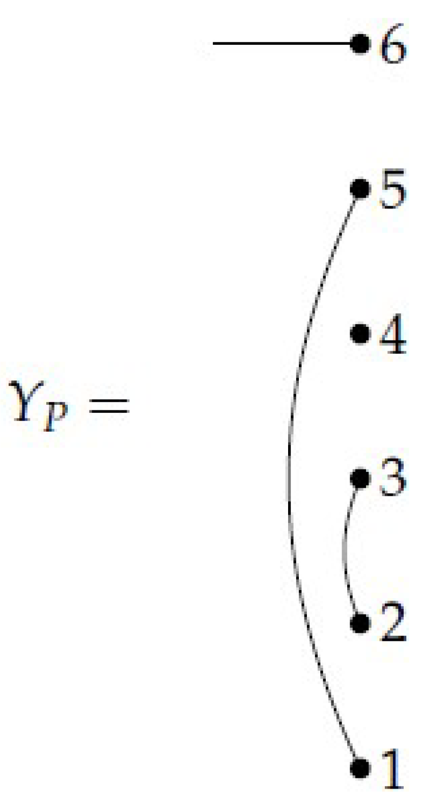
Let be a diagram obtained from the right-link state by making all defects into left-to-right horizontal connections. For ex, if and , then
Note that where is a fixed nonnegative integer. Assume first that is nonempty, then any diagram in has a right-to-right connection or isolated node labeled by i.e these connections or isolated nodes are outside the connection . This implies right-multiplying by takes into and this induces the map
Since there is no such that , any diagram in has to have a right-to-right connection or isolate node labeled by and hence, we have an inclusion . Along with the inclusion , these induce the map
The map induced by right-multiplying by is surjective because for any diagram , . Since , this maps also splits with the splitting map
If , then and we also have because of the assumption that no right-to-right connections or isolated nodes labeled by inside the connection x to y so . The same map as above implies that is a direct summand of . □
Figure 6.
and .
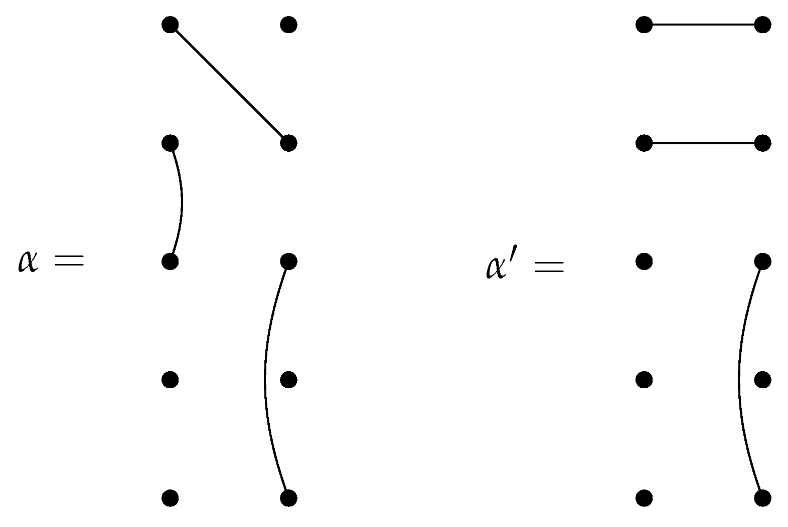
Figure 7.
and .

Similar result holds for and .
Lemma 5.
Let be invertible.
- Let . Then and is a direct summand of .
- Let with . Then .
Proof.
To show that , it suffices to show that . This follows because for any diagram . The proof that is a direct summand of mirrors that of Lemma 2 with replaced by . It suffices to show . Any diagram in has x connected to some element which implies for some partition P containing . The result then follows because by the proof of Lemma 4. □
Analogue of Lemma 1 also holds with identical proof where is replaced by .
Lemma 6.
In particular,
for all .
Let J be a left ideal of that is included in . Then
We also have a similar resolution of in terms of and .
Proposition 3.
Let , let , and assume . The following sequence, in which all maps are induced by either an inclusion or an identity map, is a resolution of .
 Moreover, applying to the sequence gives a resolution of .
The proof of this proposition is identical to that of Lemma 2 with replaced by , Lemmas 5 and 6 in place of Lemmas 2 and 1, respectively.
Lemma 7.
induced by inclusion maps is an isomorphism of left -modules where the outermost direct sum runs over all ; with y fixed, the inner sum runs over all partitions P of (or if ) into subsets of size at most 2 such that .
Let with , then the map
Proof.
Since , is sent into . Since , diagrams in have node y connected to node x so these diagrams are also in and is sent into . The map above is well-defined following from these facts.
To see that the map is surjective, any diagram in has a right-to-right connection from node x to another node . Inside this connection, there might be more right-to-right connections which, taken all together, can be identified with a partition P of (or ) into subsets of size at most 2 such that . Hence, the diagram is in the image of the direct summand with the specified y and P above so the map is surjective.
To see that the map in injective, note that two diagrams from different direct summands ’s have to be distinct in . This is because for different y’s, node x of the two diagrams is connected to two different nodes so the diagram can’t be the same. When y’s are the same, different partitions P’s of (or ) yields different right-to-right connections inside the right-to-right connection of node x and y and hence, two diagram also can’t be the same as well.
Therefore, to show that the map is injective, it suffices to show that for each direct summand , the map is injective. This is clear because in order for a diagram in to be zero in , there must be at least a right-to-right connection or an isolated node among nodes of labeled by . Since has node x connected to node y, this implies that the right-to-right connection or isolated node must occur among nodes of labeled by . But this implies in . □
We are now fully equipped to establish the analogue of Theorem 4 in the context of Motzkin algebras.
Theorem 5.
For invertible and any , let , then the groups vanish in positive degrees.
Proof.
The proof of this is almost identical to that of Theorem 4 with the following changes:
- Replace all by .
- Replace Proposition 2 by Proposition 3.
- is a direct summand of by Lemma 5.
- By Lemma 7, is a direct sum of ’s and by Lemma 4, is a direct summand of where with .
□
5. Proof of Main Results
In this section, we present the proofs of our main results, Theorem 1 and Theorem 2. We give the proof of Theorem 2 first as it is an immediate consequence of Theorem 5.
Proof of Theorem 2 For invertible and any , we can apply Theorem 5 with to yield for . Since is spanned by permutation diagram namely the identity diagram, we see that as a left -module, is isomorphic to the trivial module, . This implies for and it’s also clear that . □
To prove Theorem 1, we need the analogue of Shapiro’s Lemma for the Rook-Brauer algebras.
Theorem 6.
Let . Suppose ϵ is invertible in R and , then the maps
and
are mutually inverse isomorphisms.
We can see that Theorem 1 follows immediately from Theorem 6 by choosing and noting that and . For the rest of this section, we will establish preliminary results to prove Theorem 6.
Recall from Def 7 that denotes the left ideal spanned by all diagrams in which among the nodes on the right labeled by , there is at least one singleton or a right-to-right connection. Furthermore, is also a right -module via the inclusion and this implies is a right -module.
Lemma 8.
For , is free when regarded as a right -module.
Proof.
Any nonzero diagram in has no singleton or right-to-right connection among nodes in i.e each node in is connected to a distinct node. These diagrams form a basis of as a right R-module and since acts freely on these diagram, is a free -module. □
Lemma 9.
For , there is an isomorphism of left -modules
where is mapped to .
The proof of this Lemma is almost identical to that of Lemma 5.3 of [1] with replaced by and replaced by .
Proof of Theorem 6: Under the assumption of Theorem 6, we have
by Theorem 4. The proof now follows exactly as that of Theorem 4.1 of [3] with replacing and using Lemma 9, Theorem 4 in place of Lemma 4.4 and Theorem 3.2, respectively. □
References
- Rachel Jane Boyd, Richard Hepworth, and Peter Patzt, The homology of the partition algebras, Pacific Journal of Mathematics 327 (2023), no. 1, 1-27, available at https://msp.org/pjm/2023/327-1/p01.xhtml.
- Rachel Jane Boyd and Richard Hepworth, The homology of the Temperley-Lieb algebras, Geometry and Topology 28 (2024), no. 3, 1437-1499, available at https://msp.org/gt/2024/28-3/gt-v28-n3-p11-s.pdf.
- Rachel Jane Boyd, Richard Hepworth, and Peter Patzt, The homology of the Brauer algebras, Sel. Math. New Ser. 27 (2021), no. 85, available at https://link.springer.com/article/10.1007/s00029-021-00697-4.
- Guy Boyde, Idempotents and homology of diagram algebras, Math. Ann. 391 (2025), 2173–2207, available at https://link.springer.com/article/10.1007/s00208-024-02960-3.
- Peter Patzt, Representation stability for diagram algebras, Journal of Algebra, vol 638 (2024), 625-669. [CrossRef]
- Andrew Fisher and Daniel Graves, Cohomology of Tanabe algebras (2024), available at https://arxiv.org/abs/2410.00599.
- Cohomology of diagram algebras (2024), available at https://arxiv.org/abs/2412.14887.
- Minoru Nakaoka, Decomposition Theorem for Homology Groups of Symmetric Groups, Annals of Mathematics, vol 71 (1960), 16-42, available at https://www.jstor.org/stable/1969878.
- Anthony Muljat and Khoa Ta, Noetherianity of Diagram Algebras (2024). [CrossRef]
Disclaimer/Publisher’s Note: The statements, opinions and data contained in all publications are solely those of the individual author(s) and contributor(s) and not of MDPI and/or the editor(s). MDPI and/or the editor(s) disclaim responsibility for any injury to people or property resulting from any ideas, methods, instructions or products referred to in the content. |
© 2025 by the authors. Licensee MDPI, Basel, Switzerland. This article is an open access article distributed under the terms and conditions of the Creative Commons Attribution (CC BY) license (http://creativecommons.org/licenses/by/4.0/).
Copyright: This open access article is published under a Creative Commons CC BY 4.0 license, which permit the free download, distribution, and reuse, provided that the author and preprint are cited in any reuse.


