Submitted:
28 May 2025
Posted:
29 May 2025
You are already at the latest version
Abstract
In the production process of plate, the main factors affecting the yield of plate are the crop cutting and edge losses It is very important to accurately predict the crop pattern of plates and effectively control the plan view pattern. In this paper, a detection scheme is proposed to obtain plan view pattern of intermediate slab and finished plate by placing the detection devices after roughing mill and finishing mill respectively. The image processing algorithm is used to obtain the dataset of plan view pattern parameters, and the plan view pattern prediction and control model of plate is established based on BWO-DNN algorithm. The BWO algorithm is used to optimize the hyperparameters in DNN algorithm to complete the establishment of the intelligent model. In terms of model analysis, goodness of fit (R2) and mean absolute error (MAE) are used as evaluation indicators. The results show that the intelligence model established based on BWO-DNN has good predictive and control performance, realizing intelligent prediction of the crop pattern of plates and parameters optimization of plan view pattern control. The actual production verification on site shows that the irregular area of plate head and tail can be reduced by 17.2 % and 22.6% respectively.
Keywords:
plate
; PVPC
; intermediate slab
; machine learning
; BWO-DNN
1. Introduction
Plates, as important steel materials, are widely used in infrastructure construction and mechanical manufacturing [1]. The yield of plates is an important economic and technical indicator for evaluating enterprises' resource utilization and competitiveness. The main influencing factors of the yield is the shear loss caused by the restriction of the plan view pattern [2]. Plate plan view pattern control (PVPC) is a very effective method to make the plate rectangular, reduce crop and edge losses, and improve the yield. Its basic idea is to predict the pattern of the rolled piece after rolling, and convert the volume of the irregular pattern into an abnormal thickness compensation amount given in the last pass of the sizing and broadening phase according to the "constant volume principle". This abnormal thickness distribution is used to improve the final rectangularity. The basic principle of the plan view pattern control is shown in Figure 1.
Extensive research has been conducted by scholars on plan view pattern control. Early studies primarily adopted mechanism models, deriving theoretical equations for three-dimensional metal flow and spreading through basic laws such as the equal volume method and the minimum resistance method. These models provided a foundational basis for analyzing the plan view pattern of plates. For example, Ding [3] established a mathematical model for the plan view pattern of plates to explore the variation law of deformation parameters during the rolling process. Liu [4] used the energy method to develop an accurate prediction model for plate rolling. However, mechanism models often exhibit substantial errors due to the simplification and assumptions of physical phenomena. In contrast, the finite element analysis method can accurately predict stress, strain, and temperature distributions through fine discretization, adapting to material nonlinearity and complex boundary conditions. This not only enhances the accuracy of plan view pattern control but also provides more reliable support for optimizing process parameters.
Hu and Zhang [5,6] established plan view pattern control models for plates based on simulation and proposed new technologies such as the THP edge-free rolling process to improve slab yield. Xun [7] employed the elasto-plastic finite element method to analyze the influence of rolling conditions on the plate plan view pattern, proposing a calculation formula for the plan view pattern curve. Yang et al [8] established a plan view pattern prediction model based on the longitudinal length difference at plate head and tail, improving prediction accuracy through the relationship between metal volume and length difference, and verified the model's effectiveness through finite element simulation and experiments. Ding et al [9] studied the influence of setting points and distances on the rectangularity of products using a controllable point set-ting method combined with finite element analysis, successfully increasing the pro-duction yield from 92.28% to 93.36%. Yin [10] analyzed metal flow through simulating the rolling process, compared the plan view patterns under different rolling schedules, and obtained a comprehensive optimal rolling schedule. Masayuki Horie [11] et al. studied the dog-bone rolling method and found that the dog-bone width and broadening ratio significantly influence the plastic deformation length and fish-tail length. When the width increases or the broadening ratio decreases, the fish-tail length in-creases. Gu [12] used the finite element method to study the control of plate plan view pattern by flat and vertical rolls, proposed a theoretical model, and the simulation results matched the actual situation, reducing the difference in width elongation and effectively controlling the head convex shape. Wang [13] analyzed the variation law of plate plan view pattern through finite element modeling, and improved the width accuracy by 27% after parameter optimization. Yao [14] et al. established a prediction model and control model for plan view pattern control of wide plates based on the constant volume law, and applied the models on site, reducing the shear loss of products.
With the vigorous development of intelligent technologies, research on plate plan view pattern has been integrated with advanced technologies such as machine learning and machine vision. Machine vision detection technology [15] is rapidly emerging in the industrial field, gradually replacing human eyes for measurement and judgment. Chen et al [16] proposed a new strip shape recognition method, optimizing neural networks with orthogonal polynomials and binary trees to construct a hybrid model and improve recognition accuracy. Ma [17] studied the selection of industrial cameras and image processing algorithms to realize online real-time recognition of plate con-tours and accurate positioning of crop positions for head and tail. He et al [18] used improved image processing algorithms based on machine vision technology to re-al-time detect the position and angle information during the steel turning process, enabling real-time processing of detection data in complex production environments. Ding et al [19] employed machine vision to measure the camber of plates, obtaining sub-pixel coordinates of the rolled piece edges and determining their plan dimensions to implement feedback control for camber defects. Yang [20] achieved high - precision recognition and contour feature extraction of plates based on machine vision technologies such as binocular multi - group linear array cameras.
Machine vision technology combined with machine learning algorithms can analyze and process massive data and image information to realize monitoring, prediction, correction, and optimization of plate deformation, defects, and plan view patterns. Machine learning models aim to tap the potential in feature extraction and model construction for plate plan view patterns, deepening the intelligent research on plan view pattern control. Wang [21,22] built BP neural networks to establish metal rolling flow prediction models, though they faced challenges such as data deviation and long computation times. M.S. Chun [23] established a multi-layer neural network model to predict width changes during plate rolling, determining the optimal broadening value to reduce edge trimming losses. Dong [24] developed an ISSA-ANN plan view pattern prediction model based on on-site production data, optimizing initial weights and thresholds to overcome the problem that the traditional neural network was easy to produce local optimum. Jiao et al [25] optimized the RBF neural network by using DBO algorithm, and developed a prediction and control model for plate plan view pattern. In practical on-site applications, the crop cutting loss area of irregular deformation in the plate can be reduced by 31%. Wu et al [26] proposed an attention-based weight-adaptive multi-task learning framework for predicting and optimizing irregular shapes in hot rolling, optimizing the short-stroke process to achieve a 10.3% improvement in defect width deviation. Zhao [27] studied the application of extreme learning machines in predicting the length of rolled pieces, optimizing the prediction model for the plate plan view pattern.
Currently, research work on intelligent optimal control of plate plan view pattern using machine vision inspection is based on pattern inspection of finished plates at the end of rolling. However, passes for plan view pattern control occur in the rough rolling stage, specifically at the final pass of sizing phase and broadsiding phase. Due to requirements of TMCP rolling process for plates, there is a holding temperature process after rough rolling stage. Multiple rolled pieces will first complete rough rolling stage and holding temperature before proceeding to subsequent rolling passes to become products. Therefore, product pattern detection results can not be followed by a rolled pieces for real-time correction, plan view pattern control optimization has a large lag. If an accurate description of final shape can be obtained immediately after the end of rough rolling, plan view pattern of next piece can be optimized and adjusted in time.
Based on above background, by reasonably arranging detection devices, intermediate slab plan view pattern of rolled piece can be obtained after rough rolling. Then, according to subsequent rolling process conditions, machine learning algorithms can be used to predict the final shape in advance, enabling timely feedback and optimization of plan view pattern control for next rolled piece. Existing actual data from product shape detection serves as both machine learning data source for model predicting final pattern from intermediate pattern and evaluation tool for the final control effect.
This paper takes a typical two-stand plate production line as the research object, deploying visual detection devices after both rough mill and finish mill to collect intermediate slab and final plate plan pattern data during rolling. Using intermediate slab pattern data and subsequent rolling schedule data as inputs, and corresponding final pattern prediction is obtained through machine learning algorithm as output result. Based one final pattern prediction, we evaluate effect of plan view pattern control and optimize control parameters, and optimize plan view pattern of subsequent rolled piece in real time. The actual measurement data of final plate pattern serves as ultimate evaluation for prediction and control models.
2. Data Acquisition
2.1. Industrial Camera Settings
In order to obtain plan view pattern measured data of intermediate slab and plate, industrial camera was installed at the exit of rough rolling mill and finish rolling mill for image acquisition, as shown in Figure 2. Industrial camera 1 was installed at the exit of the rough rolling mill to collect the plan view pattern image of intermediate slab, and industrial camera 2 collects plan view pattern image of the finished plate.
2.2. Intermediate Slab Detection
After the rough rolling stage, PVPC pass rolling was completed. Plan view pattern of plate can be predicted in advance by using plan view pattern of intermediate slab and subsequent rolling schedule. The image of intermediate slab head and tail after rough rolling was collected by industrial camera, and the image of intermediate slab was grayed, and then the projection transformation was performed to obtain gray image at the top view angle, as shown in Figure 3. This operation was convenient for subsequent better identification of intermediate slab head and tail and extracted the characteristics of intermediate slab.
In order to more accurately find intermediate slab and plate head and tail shear line, it is necessary to get accurate and clear images first. Due to the different temperatures of plates in different passes and the different light and darkness of the workshop at different times, the brightness of images will be affected, and it is not possible to accurately segment each plate image, which in turn affects the extraction of plate profile. Moreover, the harsh rolling environment, such as water vapor, dust and light interference, will affect the clarity of the image acquired by the measuring device, so it is necessary to use the image processing algorithm to treat the acquired image and obtain the accurate plate profile. The gray image of intermediate slab after projection trans-formation is binarized by an adaptive threshold adjustment plate image thresholding method combined with Gamma image enhancement and Canny edge extraction algorithm, and then the profile of intermediate slab head and tail is extracted. The overall process is shown in Figure 4.
2.3. Plate Profile Coordinate Points Processing
The image of plate taken by industrial camera is not all head and tail irregular area that needs to be cut, so it is necessary to further segment head and tail edge profile of the processed plate. Globally traverse the contour pixel data and connect the pixels with the same Y value on both sides. As shown in Figure 5, scan from top to bottom, find the connection line between the two points whose width is not shrinking or no longer changing as the optimal shear line, and then extract the coordinates of the segmented head-tail contour points.
When the computer collects the image contour pixel data, the upper left corner of the default image is the coordinate origin, so first of all, it is necessary to transform the coordinate origin of plate head and tail pixel coordinates. Since the starting position is randomly generated when extracting the coordinate points and the points are not averaged, in this study, the missing points will be interpolated, after which the pixel points will be transformed to the actual coordinates according to roller table drawing size. In order to facilitate statistics and data management, the contour data is equidistantly processed. On the premise of ensuring the fitting accuracy, 101 point coordinates are used to represent intermediate slab profile and plate profile respectively.
2.4. Data Pre-Processing
In the actual rolling process, the crop will show irregular asymmetry, which is because the plate in the rolling process is affected by the transverse asymmetric factors, such as the stiffness difference on both sides of the mill, the transverse temperature of the plate and the deviation of the center line of the plate. Therefore, in the actual col-lection of 101 contour points in the head-tail deformation area, the middle point is taken as the benchmark, and the y values of the left and right symmetric two points are treated as the mean value, as shown in Figure 6. Through testing, it was found that the samples with poor symmetry of plate head and tail had a great influence on the pre-diction performance of intelligent model. Therefore, data samples with head and tail symmetry rates between 0.95 and 1.05 were selected.
In this paper, the actual rolling data of plates produced from plants were selected as samples for plate plan view pattern neural network prediction model. Since the theoretical control of plan view pattern is very complicated, in the actual rolling process, the simplified model curve shown in Figure 7 is adopted under the condition of guaranteeing the control accuracy. The width center of the rolled piece is symmetrically distributed along the width direction of the plate. The control parameters are the length of the head-tail platform section L1_b, the unsteady length L2_b, the PVPC height Dh_b and the PVPC height added value G_b.
Considering the physical model and the actual production situation, 13 main features of plate are selected, combined with head-tail contour points of plate and inter-mediate slab contour points as the dataset for establishing the machine learning model. As shown in Table 1.
3. Research Method
3.1. Deep Neural Network
Deep Neural Network (DNN) is an artificial neural network with multiple hidden layers [28,29], sometimes called Multi-Layer Perceptron (MLP). Compared with traditional shallow neural networks, DNN can learn more complex feature representations and is suitable for various complex tasks. The training process of DNN can be parallelly calculated by hardware such as GPU, which greatly accelerates the training speed. DNN is divided according to the location of different layers. The internal neural net-work layer can be divided into three categories: input layer, hidden layer and output layer. As shown in Figure 8, the first layer is the input layer, the last layer is the output layer, and all the neurons in the middle are hidden layer neurons.
In the figure, X is the input feature; Y is the output feature; n is the number of nodes in the input layer, m is the number of nodes in the output layer, and in the middle are the neurons in the hidden layer. Each neuron receives input from other neurons, and changes the influence of input features on neurons by adjusting the weights. The model can achieve the approximation of complex functions and achieve the effect of universal approximation through multi-layer nonlinear hidden layer. In this paper, the DNN neural network uses the PRelu activation function, as shown in equation (1).
Equation: x is the output of the neuron input layer, and a is a positive number, but it will be constantly updated during the training process in order to better fit the data.
3.2. BWO Optimization Algorithm
Beluga whale optimization (BWO) is a novel swarm intelligence optimization algorithm, which is inspired by the life behavior of beluga whales [30]. Similar to other swarm intelligence optimization algorithms, BWO includes exploration phase and exploitation phase. In addition, the algorithm also simulates the whale fall phenomenon in the biological world, and also introduces the Levy flight strategy to enhance the global convergence of exploitation phase.
The BWO algorithm first randomly initializes a set of solutions (the position of the beluga whale), and then evaluates the advantages and disadvantages of each solution through fitness function. Then, using the predatory behavior of beluga whales, the position of each individual is dynamically updated according to the global optimal solution and the individual historical optimal solution, so as to realize the exploration and exploitation of solution space. After several iterations, the algorithm continuously optimizes the solution until the maximum number of iterations or the fitness value is stable. Finally, the current optimal solution is output as the result. The algorithm flow chart is shown in the Figure 9.
3.3. BWO-DNN Algorithm Design
In the DNN model, weights and thresholds are critical to performance. However, the final weights and thresholds are limited by initialization, so the BWO algorithm can be used to optimize this process. Its excellent search performance can find the initial weights and thresholds that make the neural network model achieve better performance.
A set of candidate solutions are randomly generated by the BWO algorithm. Each solution represents a set of values for weight and threshold. These candidate solutions are used as the initial position of the beluga whale, and then the fitness of each candidate solution is evaluated. The location is updated by simulating the predation and whale fall behaviors of beluga whale for local and global search. The algorithm iterates until the stopping condition is satisfied, and finally outputs the optimal weight and threshold configuration to improve the performance and accuracy of the DNN model and better realize the prediction performance of plate plan view pattern. The algorithm flow of BWO-DNN is shown in Figure 10.
In order to obtain a BWO-DNN model with fast convergence speed and high computational efficiency, it is necessary to determine the appropriate range interval, population size and number of iterations, and the mean absolute error (MAE) and goodness of fit (R2) are used as model performance indicators for evaluation and parameter adjustment. As shown in equation (2) and (3).
Equation: n is the number of samples in the dataset, is the actual value of the predicted variable, is the predicted value of the established model, is the mean in the sample.
According to Eq (2) and Eq (3), it can be seen that: when the mean absolute error (MAE) value is smaller, the prediction accuracy of the model is higher; the closer the goodness of fit (R2) is to 1, the stronger the fitting degree and interpretation ability of the prediction model to the dataset.
4. Result and Discussion
4.1. Establishment and Results of Plate Plan View Pattern Prediction Model
Considering the physical model and the actual production situation, in order to obtain a more accurate and robust plate plan view pattern prediction model, this paper selects the coordinate Y value of 101 contour points of intermediate slab, the thickness of intermediate slab and the target thickness as the input variables of the model, and selects the coordinate Y value of 101 head (tail) contour points of finished plate as the output variables of the model, which are combined into a dataset used to predict plan view pattern of finished products by the measured plan view pattern of intermediate slab. The network structure of the prediction model is shown in Figure 11.
In the DNN model, inappropriate number of hidden layers and hidden neurons can lead to overfitting or underfitting. According to the complexity of the task in this study, the neural network with hidden layer between 1~3 and hidden neurons between 64~256 is tested to determine the optimal DNN structure, and the batch size is taken as 128. In the process of determining the optimal neural network structure, the learning rate is set to 0.0001, the drop_out ratio is set to 0.2, and the optimization function is set to Adam-optimizer. Since the neural network is a multi-output model, this paper uses the average R2 and average MAE of the test dataset as evaluation indicators. The test results are shown in Table 2.
It can be seen from the table that when the number of hidden layers is the same, the prediction performance of DNN will improve with the increase of the number of neurons, but when the number of neurons reaches a certain level, increasing the number of neurons will lead to overfitting. By comparing the prediction results of different network structures, the best DNN network structure of plan view pattern prediction model is 103-128-256-101. After the optimal model structure is obtained, the initial weights and thresholds of the model on this basis are checked, and it is found that the range is concentrated between-0.12 and 0.12. In order to obtain the most efficient model, it is necessary to discuss the relevant parameters of BWO, so the number of populations and iterations are first determined within this range. Although increasing the number of populations and iterations can avoid the possibility of falling into the local optimal solution due to the small number of populations or failing to find the optimal solution due to the small number of iterations, the number of populations and iterations are set too large, which may lead to slow convergence and a significant increase in calculation time. Therefore, this paper sets the same random seeds through several commonly used population size and iteration times, and tests the head plan view pattern prediction model based on BWO-DNN to determine the most suitable matching parameters. The average R2 and average MAE of the test dataset of 101 output values are used as evaluation indicators. The test results are shown in Table 3.
From the prediction results in the table, when the number of populations in the BWO algorithm is set to 50 and the number of iterations is set to 150, the prediction effect is the best. In the next step, the optimal initial weight and threshold value interval are obtained by limiting the value range of the weight and threshold to obtain the optimal weight and threshold. The results of the discussion are shown in Table 4 below.
From the results in the table, when the value interval of weight and threshold is limited between-0.1 and 0.1, the best prediction performance can be obtained, so the optimal solution can be obtained in this interval. Finally, it is determined that the population number of plate plan view pattern prediction model based on BWO-DNN is set to 50, the number of iterations is set to 150, and the value interval of weights and thresholds is set to -0.1 ~ 0.1, which completes the construction of the BWO-DNN model.
Furthermore, ELM, DNN and BWO-DNN algorithms were used to train plate plan view pattern prediction model, and the prediction performance of different algorithms was compared. Figure 12 shows the distribution of R2 in the test dataset of three different machine learning algorithms. Taking the median result as the stable result of prediction, it can be seen that the BWO-DNN model has a better prediction performance and a more stabilized R2 value compared to the ELM and DNN models.
The MAE values of the median results of BWO-DNN, DNN and ELM are 1.659mm, 1.6997mm and 2.524mm, respectively. Figure 13 is the MAE value distribution of the three algorithms. It can be seen from the figure that the average absolute error distribution of the prediction results of the BWO-DNN algorithm is more concentrated, and the generalization ability of the BWO-DNN algorithm is the best.
4.2. Establishment and Results of Plate Plan View Pattern Prediction Model
Using the plan view pattern prediction model, final pattern of plate can be obtained in real-time through intermediate slab pattern detection. A neural network model is established between the irregular region of head-tail and the PVPC parameters, and the most suitable PVPC parameters are derived through adjustment and optimization. This paper selects 8 key feature variables with significant impacts on the control parameters as input and three control parameters as output to form the dataset. The network structure of PVPC model is shown in Figure 14.
Similar to the establishment process of the plan view pattern prediction model, the number of hidden layers and neurons in the network is first determined. Due to control model of the input features and output features are relatively small, the complexity is not high, choose the hidden layers between 1-3, the number of hidden neurons between 16-128 for testing, to determine optimal DNN structure, batch size is taken as 128. Subsequently, the optimal population size, iteration times, and weights and thresholds range for BWO-DNN are determined. The results are shown in Table 5, Table 6 and Table 7.
The best DNN network structure of plan view pattern control model is 8-128-3, the best combination of population size and iteration times is 30-80, and the upper and lower limits of weights and thresholds are restricted to -0.25 to 0.25.
Three algorithms, BWO-DNN, DNN, and ELM, were used to train the plate plan view pattern control model. Three models were trained together after randomly shuffling data samples each time to generate samples of training dataset for a total of seven times, the median results were selected as the stable prediction results. Figure 15 shows the scatter plots of the results predicted by different neural networks. It can be seen that the sample results predicted by BWO-DNN are closer to the standard line. The stable prediction results of the three neural networks are summarized in Table 8, where BWO-DNN demonstrates the best predictive performance, with a median R²of 0.9605 and an average MAE of 2.124 mm. The R² and MAE of L2_b are 0.9471 and 6.2758mm; The R²and MAE of Dh_b are 0.9437 and 0.0839 mm; The R² and MAE of G_b are 0.9907and 0.0109 mm.
4.3. Verification of Actual Production Data
Through the actual application of plan view pattern intelligent model in the plate production line to explore its application effect in actual production. A group of four slabs with the same specifications and process parameters from the same batch were selected, and their process parameters are listed in Table 9. After predicting irregular head shape using the developed plan view pattern prediction model, the crop cutting area was identified for further optimization.
Four slabs to be rolled were divided into two groups. The slab numbered 1-1 was rolled using the default PVPC parameters of production line, while the three slabs in the second group adopted the parameter settings from the developed PVPC intelligent model in this paper. The specific optimized parameters are shown in the following table.

Table 10.
PVPC parameter setting.
| Optimization method | Plate number | L1_b/mm | L2_b/mm | Dh_b/mm | G_b/mm |
|---|---|---|---|---|---|
| default parameter | 1-1 | 100 | 433 | 5.5 | 0.46 |
| model optimization | 2-1 | 100 | 538 | 6.51 | 0.82 |
| 2-2 | 100 | 538 | 6.51 | 0.82 | |
| 2-3 | 100 | 538 | 6.51 | 0.82 |
Using the above rolling parameters for rolling, the head-tail images of plates were collected, and contour point coordinates were extracted using the algorithm processing flow designed in Section 2 of this paper. The shape parameters of irregular areas at the head of four plates are obtained as shown in the following table.
Table 11.
Measurement results of irregular areas.
| Plate number | Sh/mm | St/mm |
|---|---|---|
| 1-1 | 1149151.99 | 871747.05 |
| 2-1 | 942693.21 | 690293.28 |
| 2-2 | 877396.25 | 661521.32 |
| 2-3 | 1034655.85 | 671400.125 |
| Average value | 951581.77 | 674404.91 |
With the data in the table, the intelligent optimization model is significantly better than traditional model for the head-tail irregular area. Figure 16 demonstrates head irregular area of two plates. The head and tail crop cutting area can be reduced by 17.2% and 22.6%, respectively.
5. Conclusions
In this paper, the plan view pattern of intermediate slab and finished plate is detected by machine vision technology to obtain the contour data. The deep neural network optimized by BWO is used to construct the intelligent optimization model of plan view pattern. The main results of this paper are as follows.
- (1)
- A scheme of arranging visual inspection devices after roughing mill and finishing mill is proposed to obtain the actual data of intermediate slab plan view pattern and finished product plan view pattern. The intelligent optimization model is used to predict the pattern of product through the intermediate pattern data, and the real-time optimization of plan view pattern control of the next rolling piece is realized.
- (2)
- The BWO-DNN algorithm is used to construct the prediction and control model of plate plan view pattern control, which has better prediction effect than the DNN algorithm. Product head profile was predicted to improve the average R2 from 0.9657 to 0.9760 and the average MAE from 2.987mm to 2.964mm. Intelligent control model, L2_b prediction, R2 value increased from 0.9446 to 0.9471, MAE value decreased from 6.9873 mm to 6.2758 mm; for the prediction of Dh_b, the R2 value increased from 0.9139 to 0.9437, and the MAE value decreased from 0.0996 mm to 0.0839 mm. For the prediction of G_b, the R2 value increased from 0.9862 to 0.9907, and the MAE value decreased from 0.0122 mm to 0.0109 mm.
- (3)
- The developed intelligent model of plate plan view pattern control is verified in field production. Compared with the conventional model, the irregular area of head is reduced by 17.2 %. The irregular area of tail is reduced by 22.6 %.
Author Contributions
Conceptualization, Z.Z. C.H. and Z.J.; methodology, Z.Z., C.L., and J.W.; software, Z.W. (Zhiqiang Wang) and C.L.; validation, C.L. and J.W.; formal analysis, J.L. and Z.W. (Zhiqiang Wang); investigation, Z.Z. and Z.W. (Zhiqiang Wu); data curation, J.L. and Z.W. (Zhiqiang Wu); writing—original draft preparation, Z.Z., C.L., and J.W.; writing—review and editing, Z.Z., and Z.J.; visualization, J.L. and Z.W. (Zhiqiang Wang); supervision, C.H. and Z.J. All authors have read and agreed to the published version of the manuscript.
Funding
This research was funded by the Fundamental Research Funds for the Central Universities (No.: N160704003; N170708020; N2107007).
Institutional Review Board Statement
Not applicable.
Informed Consent Statement
Not applicable.
Data Availability Statement
The original contributions presented in this study are included in the article. Further inquiries can be directed to the corresponding author.
Conflicts of Interest
The authors declare no conflicts of interest.
References
- Wang, G.D. China Plate Rolling Technology and Equipment. Metallurgical Industry Press, Beijing, 2009; pp. 105–110. [Google Scholar]
- Wang, G.D. Status and prospects of research and development of key common technologies for high-quality heavy and medium plate production[J]. Steel Rolling 2019, 36(01), 1–8+30. [Google Scholar] [CrossRef]
- Ding, X.K.; Yu, J.M.; Zhang, Y.H.; et al. Establishment of Mathematical Models for Plan View Pattern Control of Plate[J]. Iron and Steel 1998, (02), 35–39. [Google Scholar] [CrossRef]
- Liu, Y.M. Research on Control Mathematical Models of Force and Shape in Plate and Strip Rolling Based on Energy Approach[D]. Northeast University, Shenyang, Liaoning, China, 2017. [Google Scholar]
- Hu, B. Physical Simulation of Plan View Pattern Control During Plate Rolling Process[D]. Yanshan University, Qinhuangdao, Hebei, China, 2006. [Google Scholar]
- Zhang, Y.H. Application Research on Intelligentized Information in Plate Production Process[D]. Northeast University, Shenyang, Liaoning, China, 2005. [Google Scholar]
- Xun, Y.W. Elastic-Plastic FEM Simulation on Plate Rolling Process[D]. Yanshan University, Qinhuangdao, Hebei, China, 2009. [Google Scholar]
- Yang, S.Y.; Liu, H. M.; Wang, D.C. Differential analysis and prediction of planar shape at the head and tail ends of medium-thickness plate rolling[J]. Metals 2023, 13(6), 1123. [Google Scholar] [CrossRef]
- Ding, J.G.; Wang, G.Q.; He, Y.H.C.; et al. Controllable points setting method for plan view pattern control in plate rolling process[J]. Steel Research International 2020, 91(1), 1900345. [Google Scholar] [CrossRef]
- Yin, X.X. Study on Plan View Pattern Control of Mid-Thick Plate by Simulation[D]. Yanshan University, Qinhuangdao, Hebei, China, 2003. [Google Scholar] [CrossRef]
- Horie, M.; Hirata, K.; Tateno, J.; et al. Influence of dog-bone width on end profile in plan view pattern control method for plate rolling[J]. Materials Transactions 2017, 58(4), 623–628. [Google Scholar] [CrossRef]
- Gu, S.F. Finite Element Simulation of the Vertical Roll and MAS Rolling in Plate Shape Control[D]. Northeast University, Shenyang, Liaoning, China, 2014. [Google Scholar]
- Wang, Q.S. Heavy Plate Plan View Pattern Control Model Study and Optimization[D]. Shanghai Jiao Tong University, Shanghai, 2007. [Google Scholar]
- Yao, X.L.; Yu, X.T.; Wu, Q.H.; et al. The application research of plan view pattern control in plate rolling[J]. Kybernetes 2010, 39(8), 1351–1358. [Google Scholar] [CrossRef]
- Zhou, J.R. Application of intelligent video recognition technology in plate production[J]. Metallurgical Industry Automation 2020, 44(S1), 254–255. [Google Scholar]
- Chen, L.J.; Han, B.; Tan, W.; et al. Technology Status and Trend of Shape Detecting and Shape Controlling of Rolled Strip[J]. Steel Rolling 2012, 29(04), 38–42. [Google Scholar] [CrossRef]
- Ma, R.W. Research on Contour Recognition and Intelligent Cutting Strategy for Wide and Heavy Plate Based on Machine Vision[D]. Shenyang Jianzhu University, Shenyang, Liaoning, China, 2021. [Google Scholar] [CrossRef]
- He, C.Y.; Xue, S.; Wu, Z.Q.; et al. Digital model of automatic plate turning for plate mills based on machine vision and reinforcement learning algorithm[J]. Metals 2024, 14(6), 709. [Google Scholar] [CrossRef]
- Ding, J.G.; He, Y.H.C.; Kong, L.P.; et al. Camber prediction based on fusion method with mechanism model and machine learning in plate rolling[J]. ISIJ International 2021, 61(10), 2540–2551. [Google Scholar] [CrossRef]
- Yang, H.; Zhou, P.; Huang, S.W.; et al. Research and Development of Intelligent Cutting System Based on Machine Vision in Medium Plate[J]. Metallurgical Industry Automation 2022, 46(01), 34–43. [Google Scholar] [CrossRef]
- Wang, Y.Y. Research and Application of Intelligent Prediction Model for Plan View Pattern of Plate[D]. Northeast University, Shenyang, Liaoning, China, 2017. [Google Scholar] [CrossRef]
- Wang, S.J. Study on Optimal Setting of Control Parameters for Plan View Pattern of Plate[D]. Northeast University, Shenyang, Liaoning, China, 2019. [Google Scholar] [CrossRef]
- Chun, M.; Yi, J.; Moon, Y. Application of neural networks to predict the width variation in a plate mill[J]. Journal of Materials Processing Technology 2001, 111(1-3), 146–149. [Google Scholar] [CrossRef]
- Dong, Z.H.; Li, X.; Luan, F.; et al. Prediction and analysis of key parameters of head deformation of hot-rolled plates based on artificial neural networks.[J]. Journal of Manufacturing Processes 2022, 77, 280–300. [Google Scholar] [CrossRef]
- Jiao, Z.J.; Gao, S.W.; Liu, C.J.; et al. Digital model of plan view pattern control for plate mills based on machine vision and the DBO-RBF algorithm[J]. Metals 2024, 14(1), 94. [Google Scholar] [CrossRef]
- Wu, W.T.; Peng, W.; Liu, J.; et al. An attention-based weight adaptive multi-task learning framework for slab head shape prediction and optimization during the rough rolling process[J]. Journal of Manufacturing Processes 2025, 133, 408–429. [Google Scholar] [CrossRef]
- Zhao, Z. Study on Dynamic Controllable Point Setting and Intelligent Optimization Strategy for Plan View Pattern Control of Plate[D]. Northeast University, Shenyang, Liaoning, China, 2018. [Google Scholar] [CrossRef]
- Das, R.; Sen, S.; Maulik, U. A survey on fuzzy deep neural networks[J]. ACM Computing Surveys (CSUR) 2020, 53(3), 1–25. [Google Scholar] [CrossRef]
- Kriegeskorte, N.; Golan, T. Neural network models and deep learning[J]. Current Biology 2019, 29(7), R231–R236. [Google Scholar] [CrossRef] [PubMed]
- Zhong, C.T.; Li, G.; Meng, Z. Beluga whale optimization: A novel nature-inspired metaheuristic algorithm[J]. Knowledge-Based Systems 2022, 251, 109215. [Google Scholar] [CrossRef]
Figure 1.
Rolling process of PVPC [25].
Figure 1.
Rolling process of PVPC [25].
Figure 2.
Industrial camera installation position installation.
Figure 3.
intermediate slab head grey image.
Figure 4.
Intermediate billet image processing flow: (a) binarization; (b) edge detection; (c) contour extraction.
Figure 4.
Intermediate billet image processing flow: (a) binarization; (b) edge detection; (c) contour extraction.
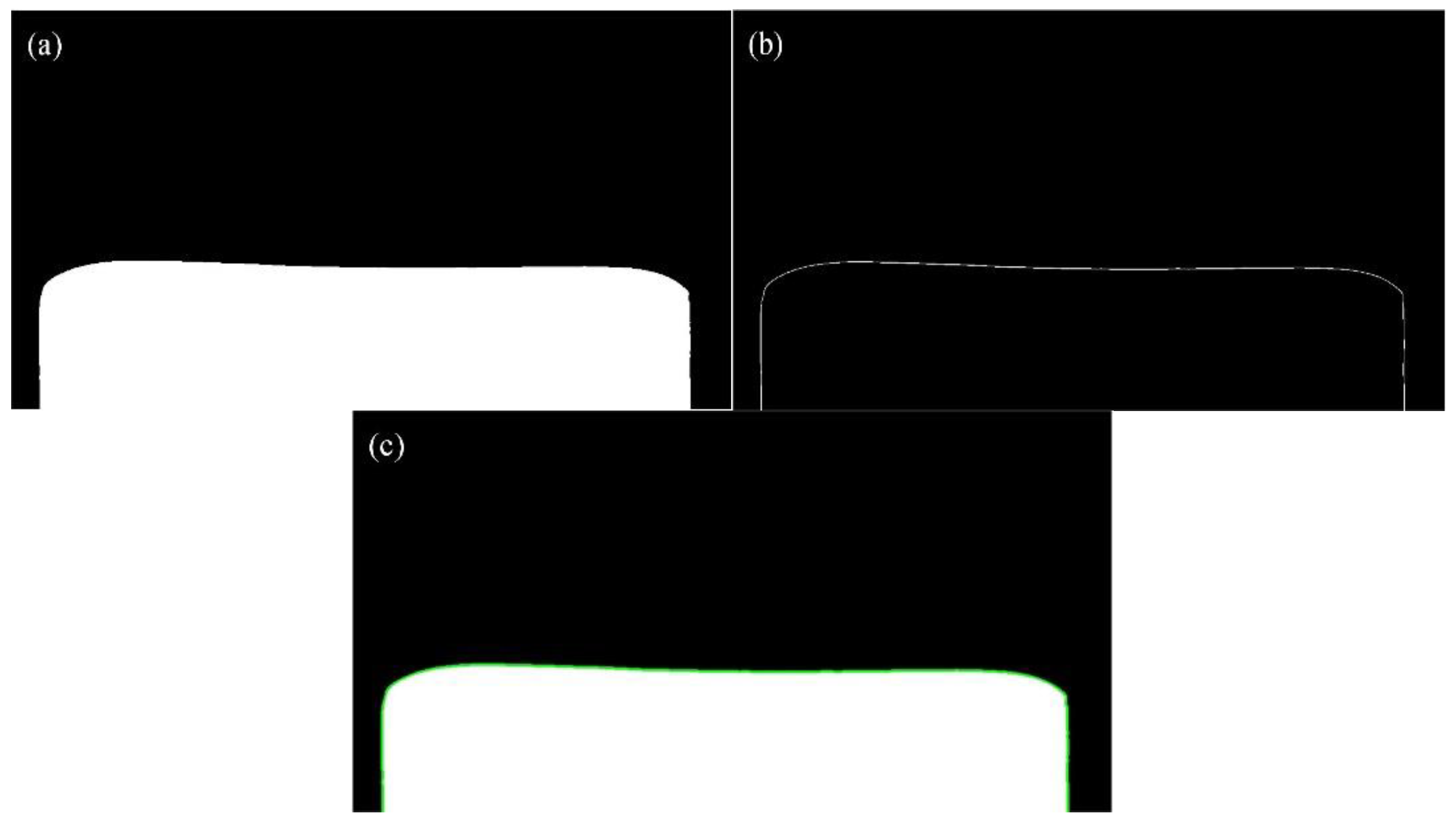
Figure 5.
Determination of the best shear line: (a) head; (b) tail.
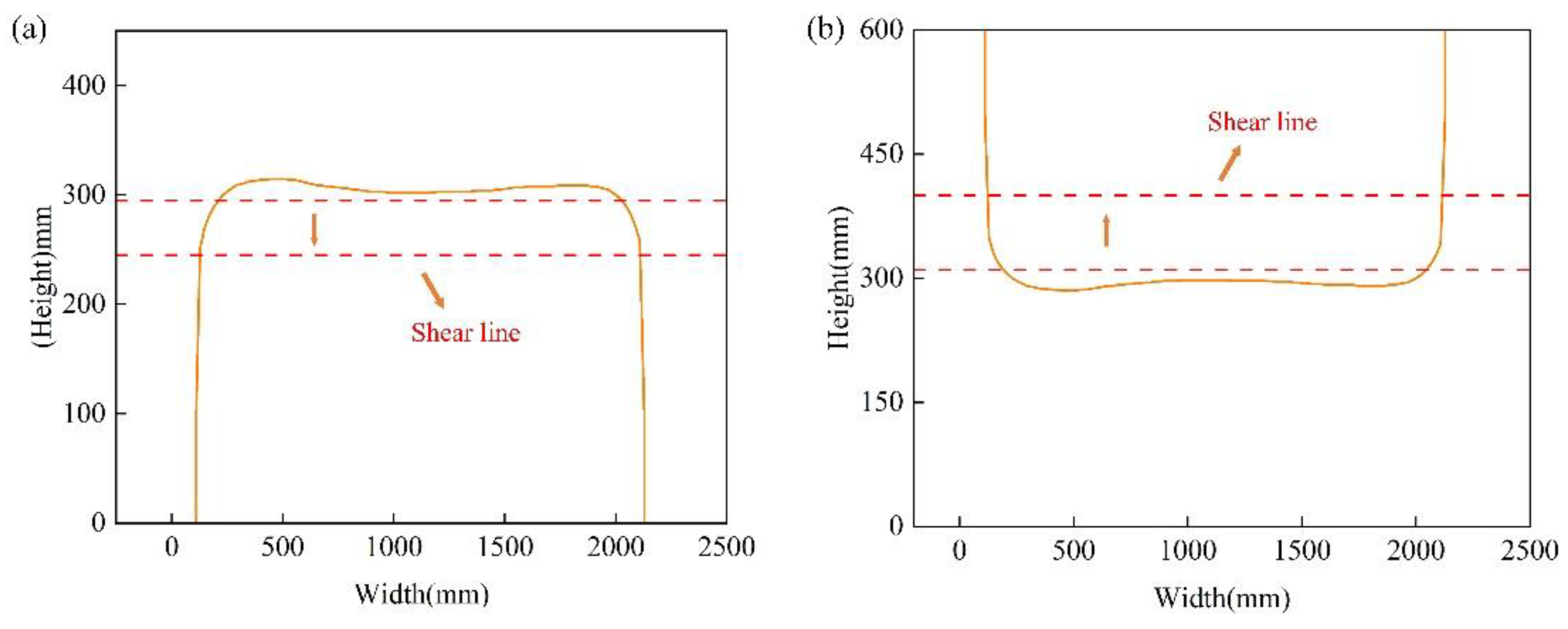
Figure 6.
Outline point coordinate processing diagram.
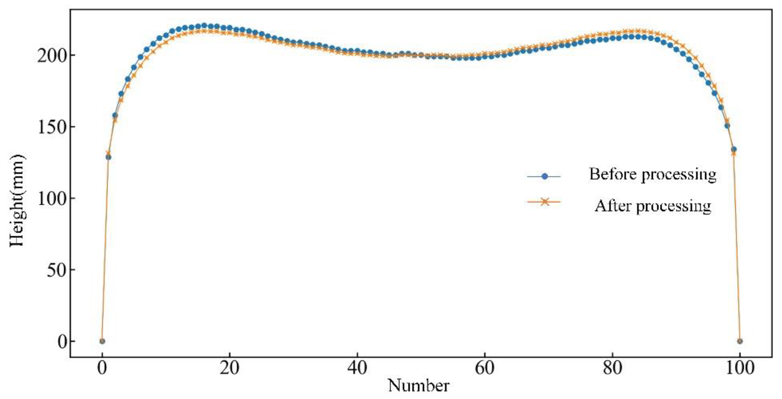
Figure 7.
PVPC diagram.
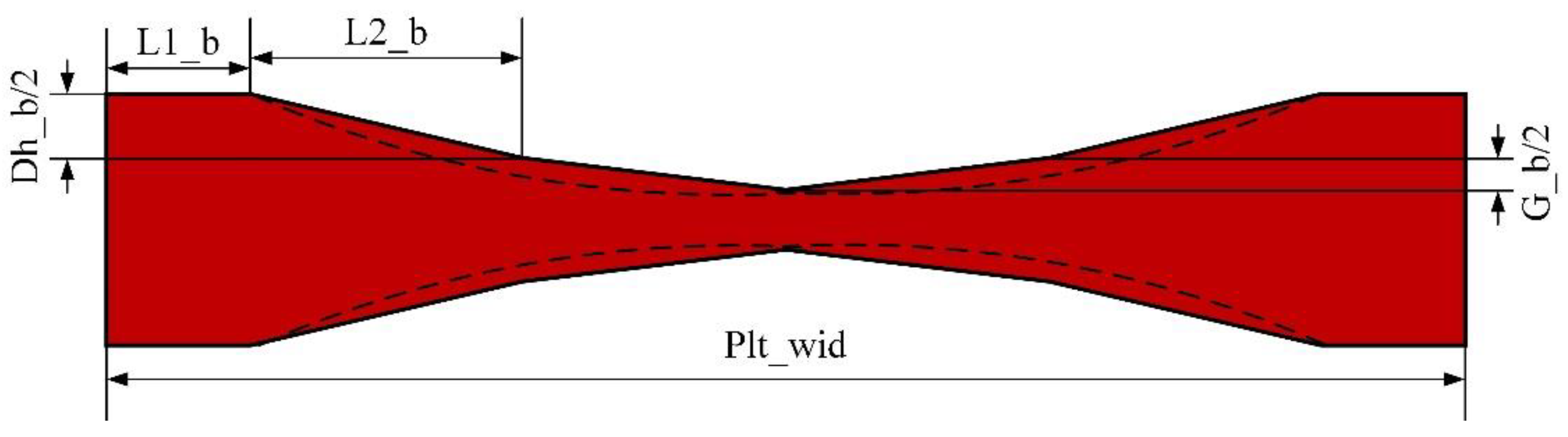
Figure 8.
DNN neural network diagram.
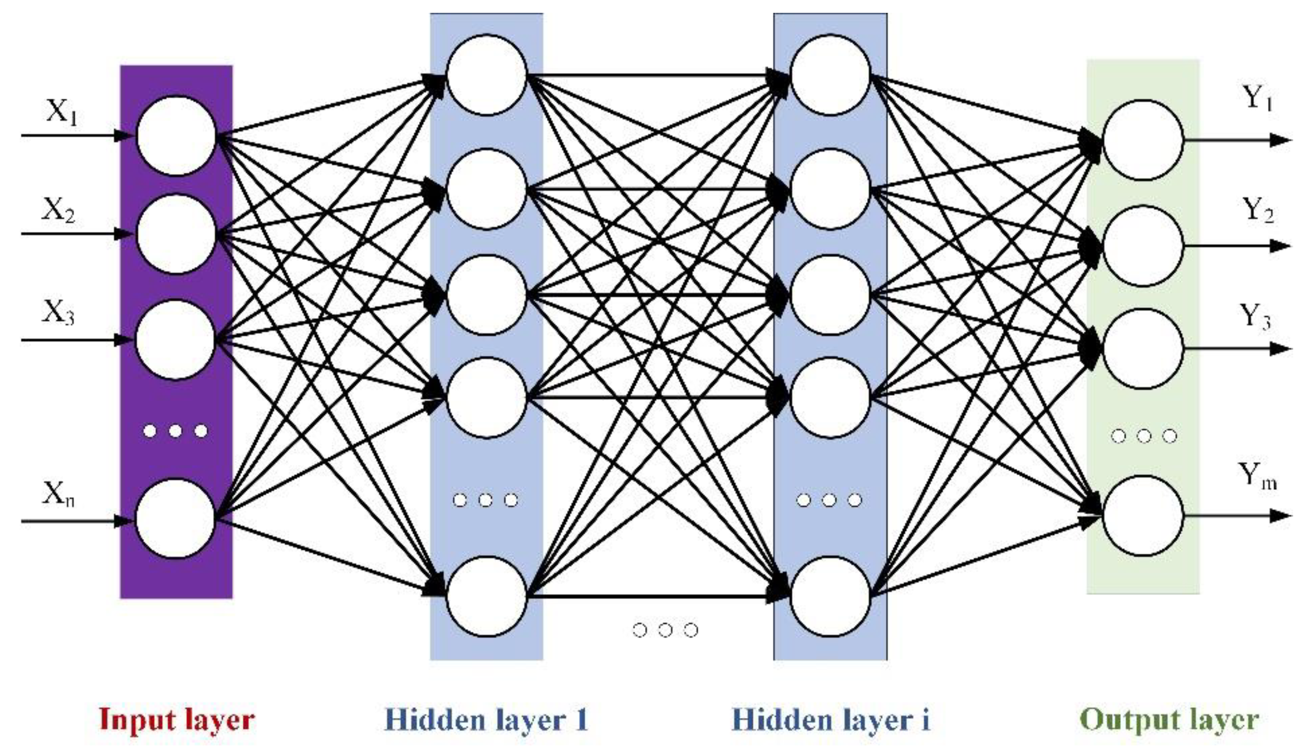
Figure 9.
BWO algorithm flow.
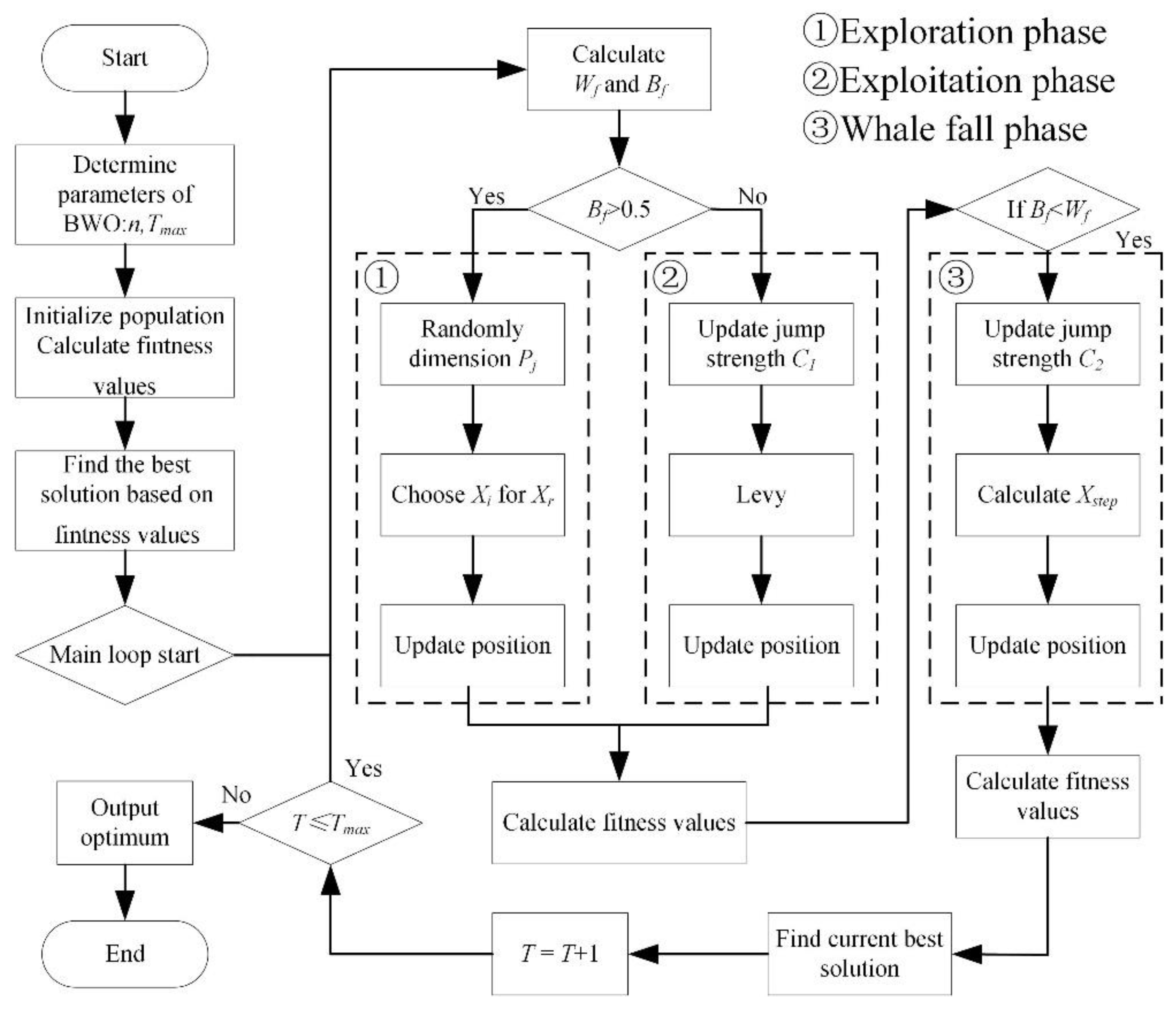
Figure 10.
DNN-BWO algorithm flow.
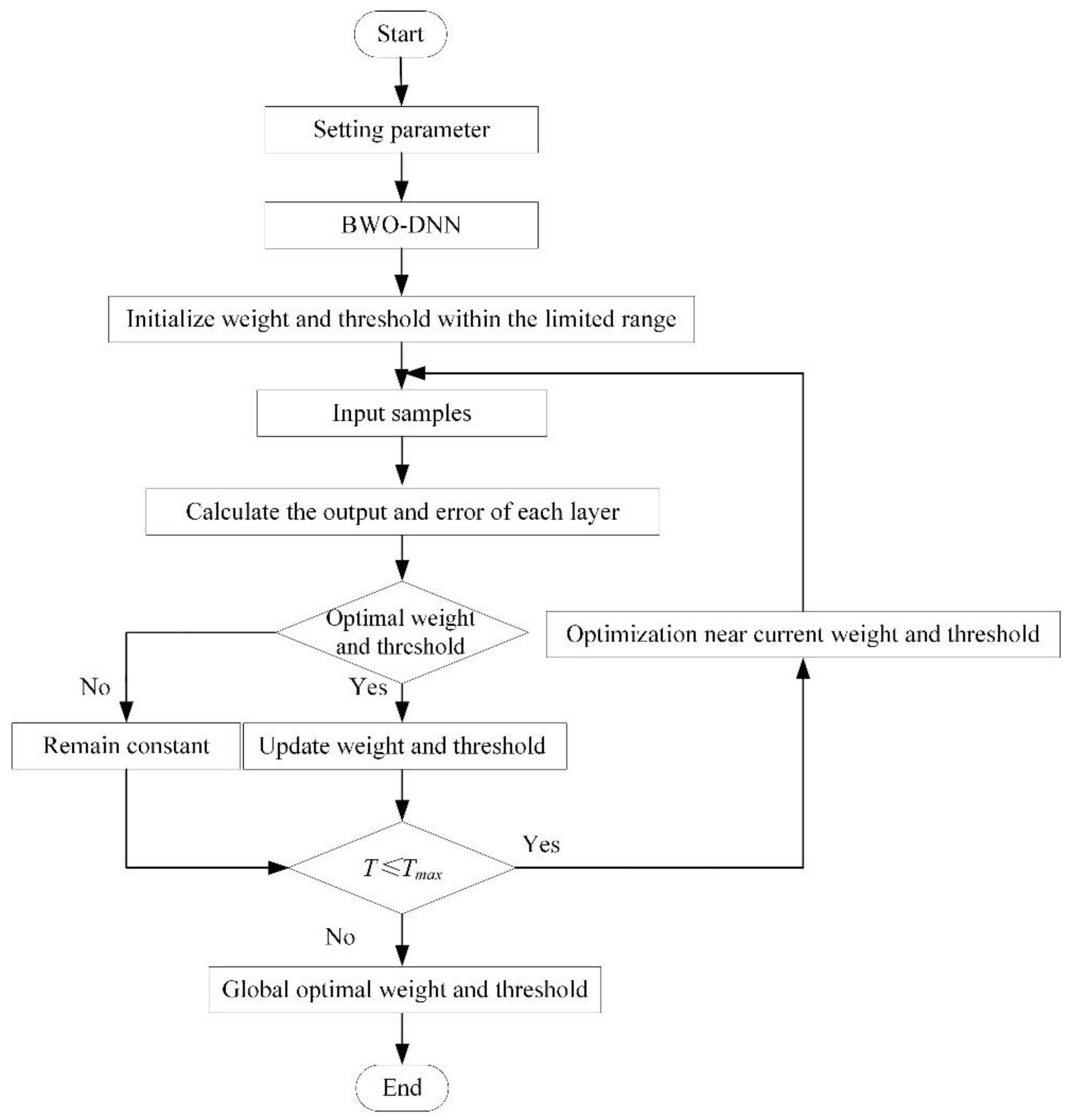
Figure 11.
Plan view pattern prediction model.
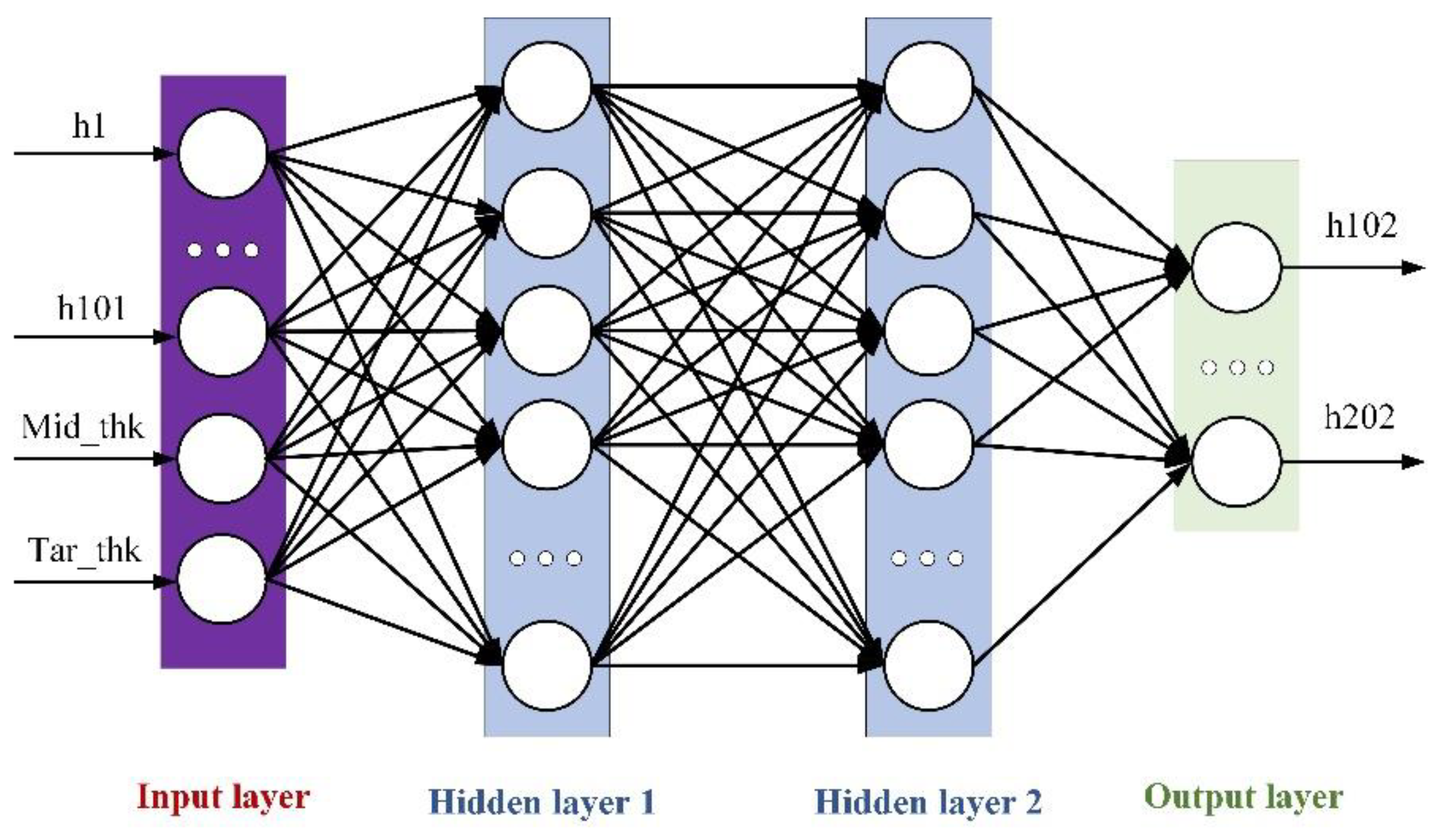
Figure 12.
The boxplot for the R2 value in multiple training sessions.
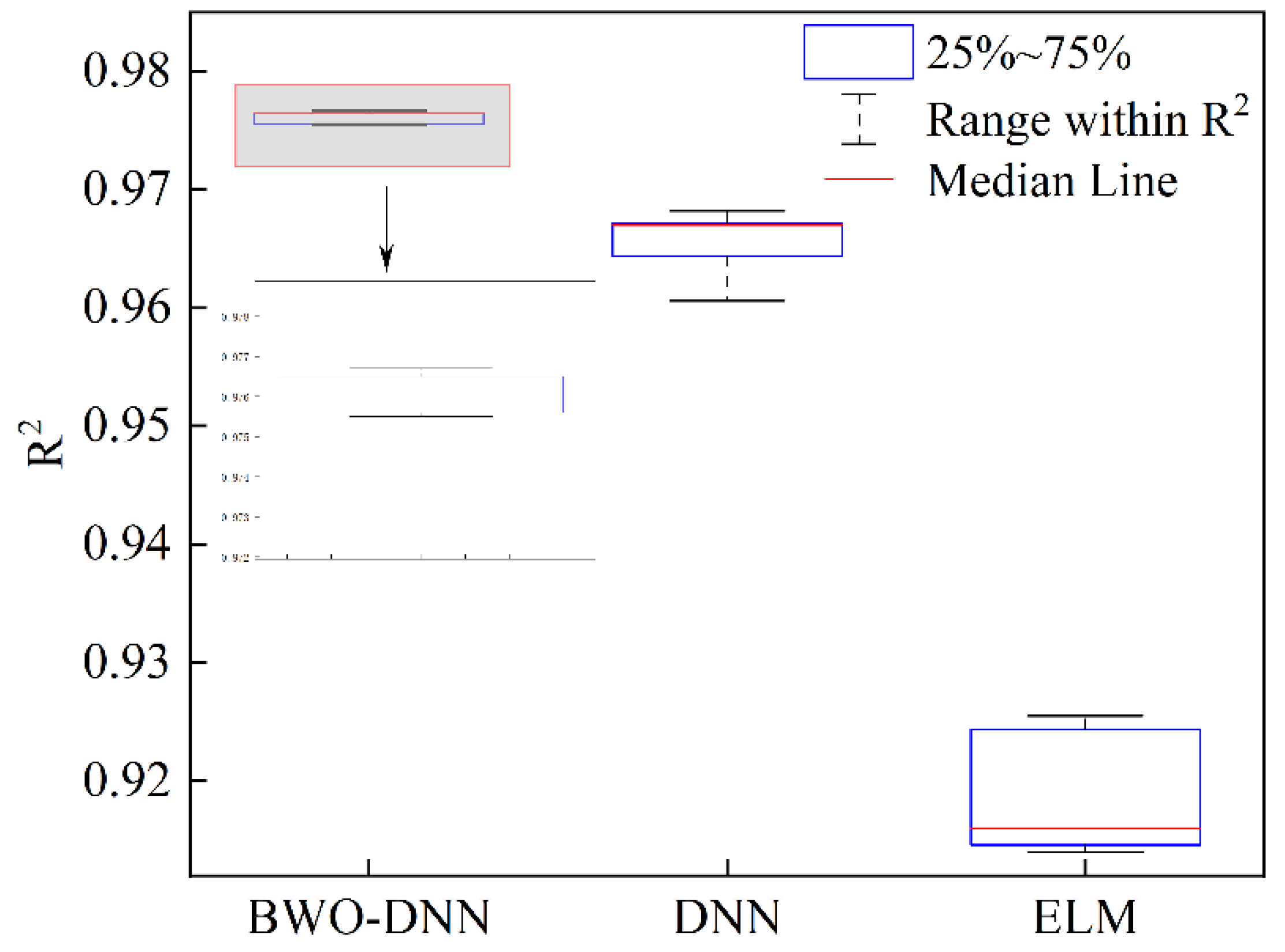
Figure 13.
MAE distribution of different algorithms.
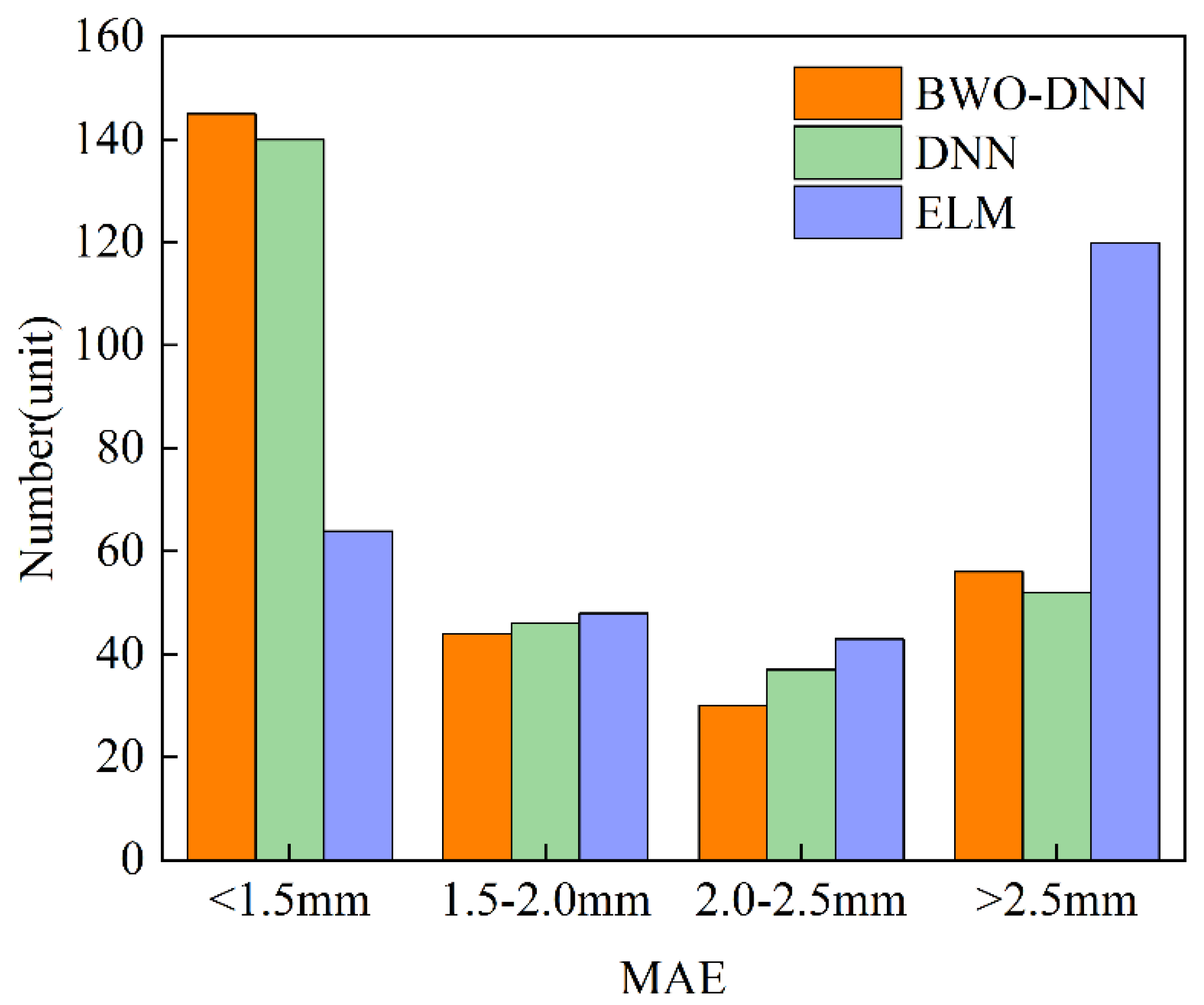
Figure 14.
Plan view pattern control model.
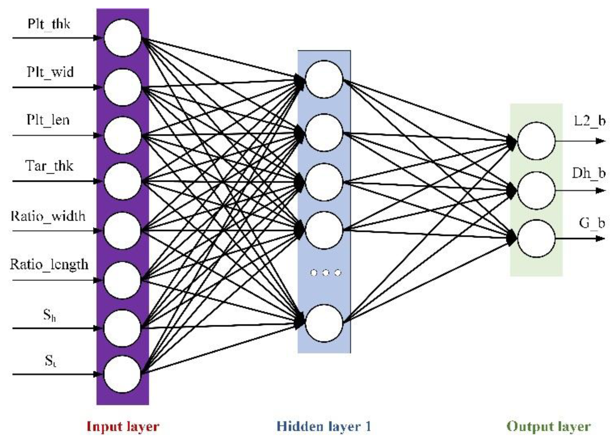
Figure 15.
BWO-DNN and DNN prediction results: (a) L2_b comparison results; (b) Dh_b comparison results; (c) G_b comparison results.
Figure 15.
BWO-DNN and DNN prediction results: (a) L2_b comparison results; (b) Dh_b comparison results; (c) G_b comparison results.
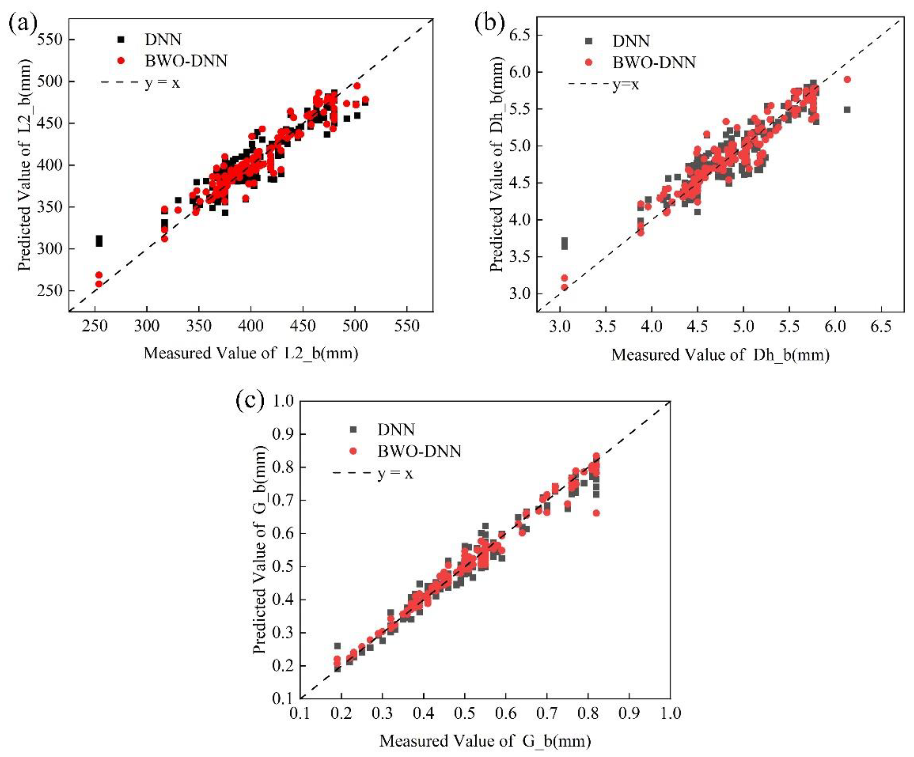
Figure 16.
Comparison of Plate Plan View Pattern Before and After Optimization: (a)Before optimization; (b) After optimization.
Figure 16.
Comparison of Plate Plan View Pattern Before and After Optimization: (a)Before optimization; (b) After optimization.
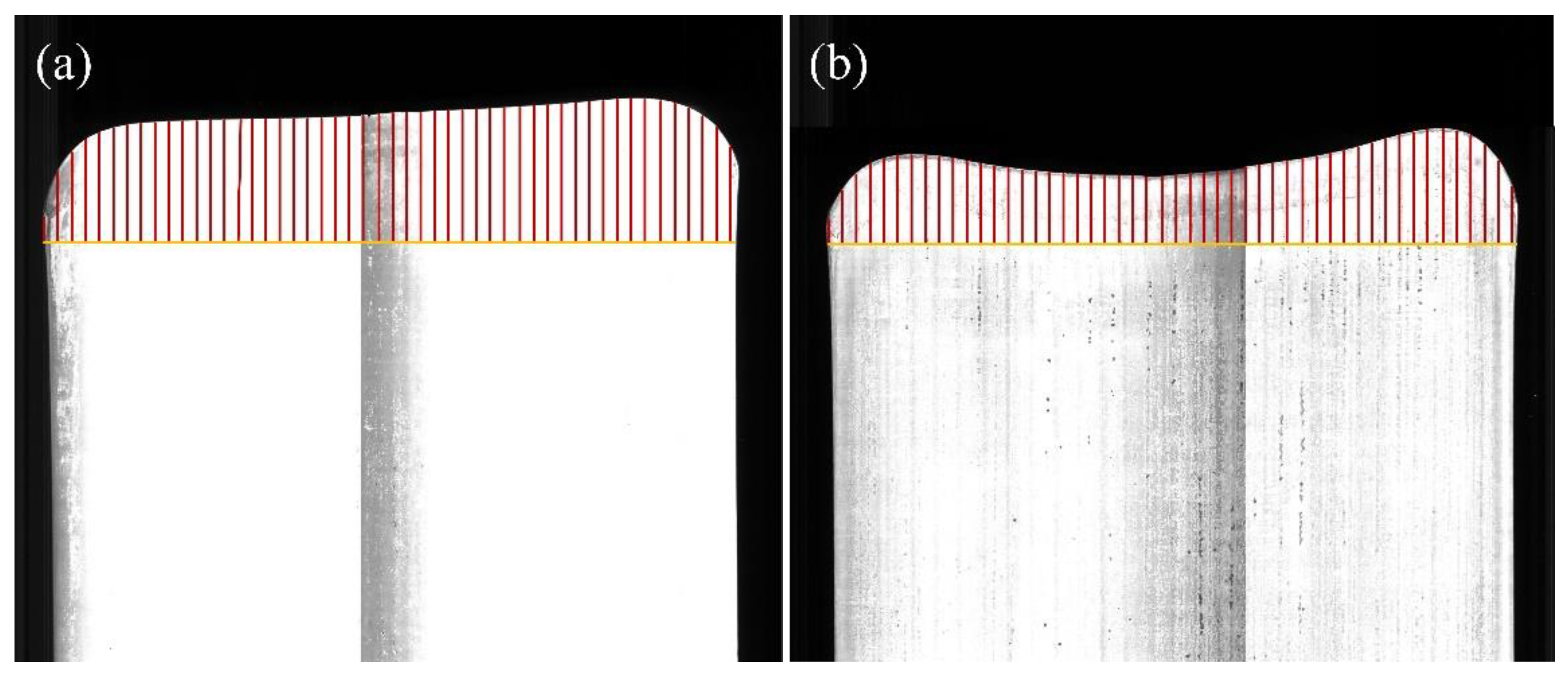
Table 1.
Data feature value summary.
| Index | Parameter | Description | Unit |
|---|---|---|---|
| V1 | Plt_thk | Slab thickness | mm |
| V2 | Plt_wid | Slab width | mm |
| V3 | Plt_len | Slab length | mm |
| V4 | Tar_thk | Target thickness | mm |
| V5 | Ratio_width | Broadening ratio after completion of rolling | - |
| V6 | Ratio_length | Extension ratio after completion of rolling | - |
| V7 | L1_b | PVPC parameter | mm |
| V8 | L2_b | PVPC parameter | mm |
| V9 | Dh_b | PVPC parameter | mm |
| V10 | G_b | PVPC parameter | mm |
| V11-V111 | h1-h101 | Y-value of intermediate slab contour points | mm |
| V112-V212 | h102-h202 | Y-value of plate contour points | mm |
| V213 | Mid_thk | Intermediate slab thickness | mm |
| V214 | Sh | Irregular area of head | mm2 |
| V215 | St | Irregular area of tail | mm2 |
Table 2.
Summary of hidden layer and neuron number discussion.
| hidden layers number | number of neurons | MAE/mm | R2 |
|---|---|---|---|
| 1 | 128 | 3.823 | 0.9436 |
| 1 | 256 | 3.214 | 0.9498 |
| 2 | 128-128 | 3.566 | 0.9496 |
| 2 | 128-256 | 2.987 | 0.9657 |
| 2 | 256-256 | 3.554 | 0.9623 |
| 3 | 100-200-300 | 3.568 | 0.9532 |
Table 3.
Effect of population size and iterations of BWO-DNN.
| population size and iterations | R2 | MAE/mm |
|---|---|---|
| 30-100 | 0.9734 | 2.981 |
| 30-150 | 0.9742 | 2.978 |
| 30-180 | 0.9750 | 2.977 |
| 50-100 | 0.9752 | 2.975 |
| 50-120 | 0.9754 | 2.971 |
| 50-150 | 0.9758 | 2.969 |
| 50-180 | 0.9758 | 2.969 |
Table 4.
R2 values of different upper and lower limits.
| value ranges | R2 | MAE/mm |
|---|---|---|
| -0.12~0.12 | 0.9758 | 2.969 |
| -0.1~0.1 | 0.9760 | 2.964 |
| -0.09~0.09 | 0.9760 | 2.964 |
| -0.08~0.08 | 0.9760 | 2.964 |
Table 5.
Summary of hidden layer and neuron number discussion.
| Hidden layers numbers | Number of neurons | MAE/mm | R2 |
|---|---|---|---|
| 1 | 32 | 1.621 | 0.9412 |
| 1 | 64 | 1.214 | 0.9431 |
| 1 | 128 | 1.206 | 0.9470 |
| 2 | 32-64 | 1.552 | 0.9423 |
| 2 | 64-128 | 1.571 | 0.9410 |
| 2 | 32-128 | 1.629 | 0.9399 |
| 3 | 32-64-128 | 1.680 | 0.9382 |
Table 6.
Effect of population size and iterations of BWO-DNN.
| Population size and iterations | R2 | MAE/mm |
|---|---|---|
| 20-50 | 0.9322 | 1.721 |
| 20-80 | 0.9389 | 1.716 |
| 20-100 | 0.9391 | 1.702 |
| 30-50 | 0.9426 | 1.627 |
| 30-80 | 0.9520 | 1.202 |
| 30-100 | 0.9520 | 1.202 |
| 50-50 | 0.9456 | 1.215 |
Table 7.
R2 values of different upper and lower limits.
| Value ranges | R2 | MAE/mm |
|---|---|---|
| -0.30~0.30 | 0.9498 | 1.362 |
| -0.28~0.28 | 0.9546 | 1.212 |
| -0.25~0.25 | 0.9569 | 1.198 |
| -0.20~0.20 | 0.9553 | 1.182 |
| -0.18~0.18 | 0.9551 | 1.213 |
Table 8.
Effect of population size and iterations of BWO-DNN.
| Parameter | Index | R2 | MAE/mm |
|---|---|---|---|
| BWO-DNN | 0.9471 | 6.2758 | |
| L2_b | DNN | 0.9446 | 6.9873 |
| ELM | 0.8805 | 11.7886 | |
| BWO-DNN | 0.9437 | 0.0839 | |
| Dh_b | DNN | 0.9139 | 0.0996 |
| ELM | 0.8583 | 0.1529 | |
| BWO-DNN | 0.9907 | 0.0109 | |
| G_b | DNN | 0.9862 | 0.0122 |
| ELM | 0.9631 | 0.0176 |
Table 9.
Summary of slab data.
| Parameter | Value |
|---|---|
| material | AH36 |
| Plt_thk/mm | 220 |
| Plt_wid/mm | 2065 |
| Plt_len/mm | 2295 |
| Tar_thk/mm | 17.65 |
| Ratio_width | 1.179 |
| Ratio_length | 10.571 |
Disclaimer/Publisher’s Note: The statements, opinions and data contained in all publications are solely those of the individual author(s) and contributor(s) and not of MDPI and/or the editor(s). MDPI and/or the editor(s) disclaim responsibility for any injury to people or property resulting from any ideas, methods, instructions or products referred to in the content. |
© 2025 by the authors. Licensee MDPI, Basel, Switzerland. This article is an open access article distributed under the terms and conditions of the Creative Commons Attribution (CC BY) license (http://creativecommons.org/licenses/by/4.0/).
Copyright: This open access article is published under a Creative Commons CC BY 4.0 license, which permit the free download, distribution, and reuse, provided that the author and preprint are cited in any reuse.


