AnnCoder: A mti-Agent-Based Code Generation and Optimization Model

1. Introduction

Code Generation, as one of the key challenges in artificial intelligence, aims to automatically convert natural language descriptions into executable code. Its applications span various domains, including Software Engineering Automation, educational tools, and complex system development, improving quality of life. To boost programmer productivity, the automation of Code Generation represents a pivotal advancement. In recent years, the emergence of Large Language Models has greatly advanced this field. Models such as Mapcoder and Self-Organized Agents [1],are paving the way for an era where fully executable code can be generated without human intervention. Nevertheless, when addressing complex logical reasoning and stringent code quality demands, existing approaches still exhibit limitations.

Early approaches utilizing LLMs for code generation employ a direct prompting approach [2], where LLMs generate code directly from problem descriptions and sample I/O. Recent methods like chain-of-thought [3] advocate modular [4] or pseudo code-based generation to enhance planning and reduce errors, while retrieval-based approaches such as leverage relevant problems and solutions to guide LLMs’ code generations [5]. Modular design improves clarity but may weaken code coherence. Current methods like MapCoder’s static case retrieval prioritize module-level improvements via historical data, yet fail to adapt to dynamic constraints. Reflexion employs test-driven iteration but fixates on pass rates, ignoring efficiency and readability. Such fragmented optimization risks local optima—minor fixes overshadowing holistic progress. Integrating multi-criteria evaluation (e.g., dynamically weighting robustness and efficiency) could unlock globally optimal solutions.

We introduce AnnCoder, a code generation model that merges multi-agent collaboration with evolutionary annealing optimization. This closed-loop framework streamlines code creation by covering case retrieval, implementation, debugging, and refinement—each managed by specialized agents. Unlike prior models that treated "generation" and "repair" as disjoint steps, AnnCoder mimics human programming’s "try-fix-adapt" cycle,like untangling a knot through persistent iteration.Key innovations include a dynamic scoring system that balances efficiency, readability, and robustness, adjusting weights like a chameleon adapting to problem types. The Evolutionary Annealing Hybrid Algorithm combines simulated annealing’s random exploration with genetic algorithms’ precision.

We evaluated AnnCoder on four popular comprehensive benchmarks for general programming, including datasets HumanEval, MBPP, HumanEval-ET, and EvalPlus.For multiple different LLMs, such as ChatGPT and GPT-4 [6]. Our method has improved the accuracy rate of code generation and performs better than powerful baselines such as Reflexion and Self-Planning.

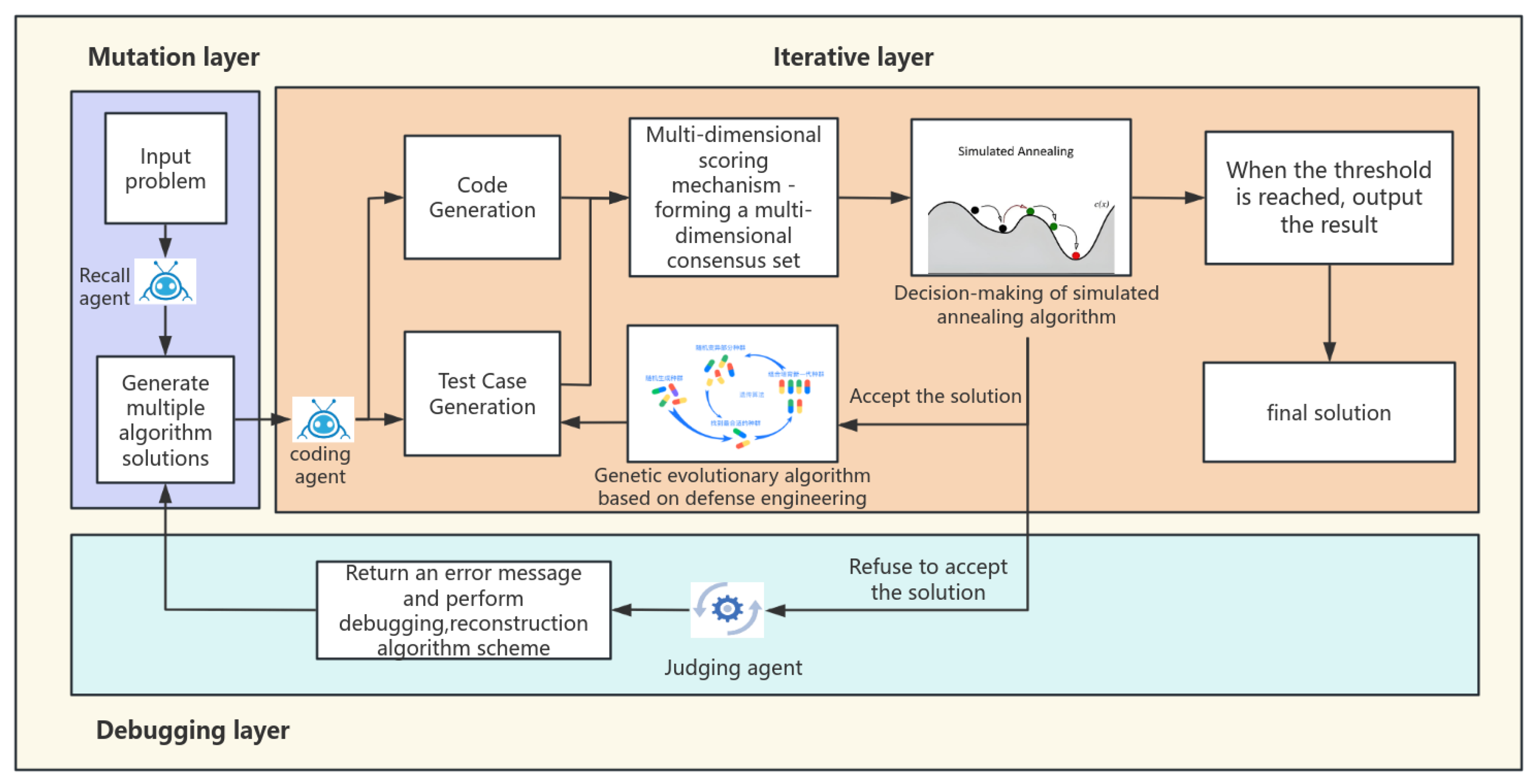
Figure 1. The comprehensive flowchart of AnnCoder.

Figure 1. The comprehensive flowchart of AnnCoder.

2. Related Work

Recently, the advent of large language models such as ChatGPT has revolutionized the domain of automatic code generation. These models have exhibited competence in tasks including code completion [7,8], code translation [9,10,11], and code repair [12,13,13], generating source code from natural language descriptions. This research domain has garnered substantial academic interest and considerable industrial attention, exemplified by the creation of tools such as GitHub Copilot, CodeGeeX [14], and Amazon CodeWhisperer, which utilize advanced large language models to enhance software development efficiency.

Initial investigations into code generation predominantly depended on heuristic rules or expert systems, including frameworks grounded in probabilistic grammars and specialized language models [15,16]. These preliminary methods were frequently inflexible and challenging to scale. The advent of large language models has revolutionized the field. Due to their remarkable efficacy and adaptability, they have emerged as the preferred choice. A notable characteristic of large language models is their capacity to adhere to commands [17,18,19], enabling novice programmers to generate code merely by articulating their requirements. This novel capability has democratized programming, rendering it accessible to a significantly broader audience.

A trend toward diversification has arisen in the evolution of large language models. Models such as ChatGPT, GPT-4 [20], LLaMA [21], and Claude 3 [22,23] are intended for general-purpose applications, while others like StarVector [24], Benchmarking Llama [25], DeepSeek-Coder [26], and Code Gemma are specifically tailored for code-centric jobs. Programming languages are increasingly incorporating the newest breakthroughs in LLMs, with these models being assessed for their capacity to fulfill software engineering requirements while also promoting the implementation of large language models in practical production settings.

Table 1. Comparison of AnnCoder with other baselines

Method	Self-Retrieval	Planning	TestCase Generation	Debugging
Reflexion	×	×
Self-Planning	×		×	×
AlphaCodium	×	×
MapCoder			×
Anncoder (Ours)

Table 1. Comparison of AnnCoder with other baselines

Method	Self-Retrieval	Planning	TestCase Generation	Debugging
Reflexion	×	×
Self-Planning	×		×	×
AlphaCodium	×	×
MapCoder			×
Anncoder (Ours)

Prompting strategies are essential for code generation and optimization. LLM prompts can be classified into three categories: retrieval [8,27,28], planning [29,30], and debugging [31]. Researchers have employed several prompting tactics, utilizing various methods to direct models in generating superior quality code. An exemplary instance is MapCoder, a traditional approach that integrates retrieval, planning, and debugging prompts with code generation. It distinctly reflects the comprehensive program synthesis cycle evident in human developers. The majority of current methodologies concentrate on fragmented optimization for a singular metric, such as the pass@k score, complicating the simultaneous improvement of functional correctness, execution efficiency, and structural quality, including symmetry. We have noticed that conventional algorithms may become ensnared in a suboptimal solution during optimization, persisting with successive improvements without reassessing the problem from a holistic viewpoint. In such instances, the algorithm may become stagnant due to inadequate investigation. Despite significant progress in this field, we argue that there is still room for further improvement.

3. Anncoder

3.1. AnnCoder Model Design

The primary objective of AnnCoder is to identify high-quality candidate solutions while circumventing the pitfalls of local optimum solutions, thereby producing code that adheres to the requirements of functional correctness, efficiency, and symmetry. AnnCoder utilizes the multi-dimensional scoring mechanism to assess solutions from several viewpoints, circumventing dependence on a singular measure to avert the inclusion of superficially accurate yet erroneous solutions in the optimization process, therefore enhancing overall performance. A hybrid algorithm that merges simulated annealing with evolutionary genetics leverages the advantages of both methodologies, significantly diminishing the probability of reaching local optimum solutions and improving the global search efficacy of independent evolutionary genetic algorithms. This section will examine the collaborative and self-enhancement processes of memory, generation, and debugging agents within the Multi-Agent Collaboration module, along with the interplay between the evolution-annealing optimization module and the multi-dimensional scoring mechanism in generating highly accurate and efficient code.

3.2. Multi-Agent Collaboration Module

3.2.1. Case Retrieval Agent

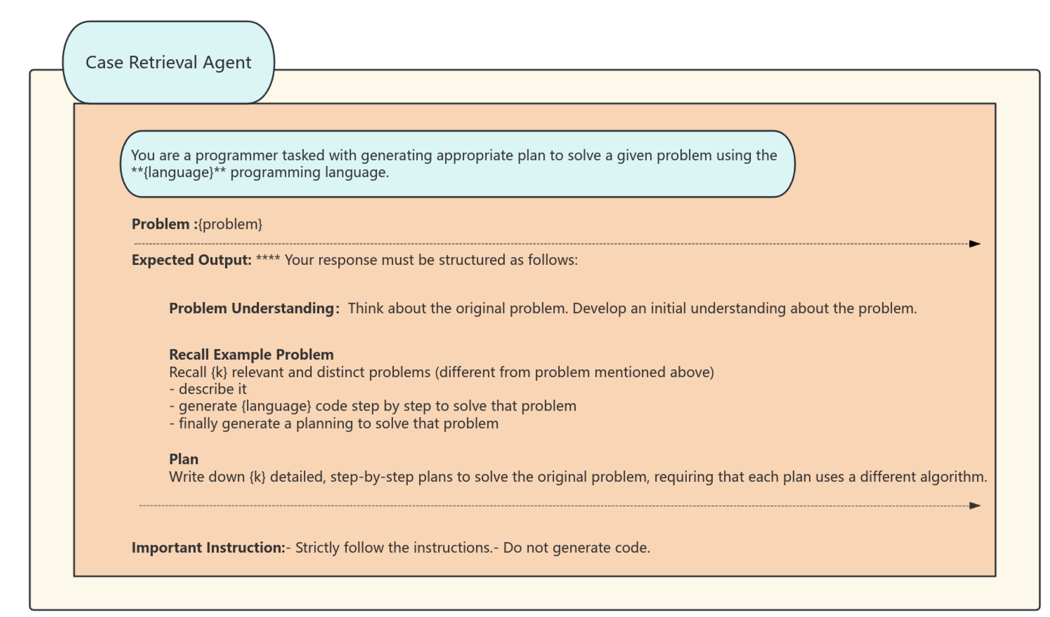
The case retrieval agent recalls past relevant problem-solving instances, akin to human memory. It finds k (user-defined) similar problems without manual crafting or external retrieval models. Instead, we leverage the LLM agent itself, instructing it to generate such problems. Our prompt extends the analogical prompting principles, generating examples and their solutions simultaneously, along with additional metadata (e.g., problem description, code) to provide the following agents as auxiliary data. We have employed a dual-layer retrieval technique, consisting of semantic embedding matching and structural pattern filtering, to accomplish this.

This intelligent agent has exceptional proficiency in cross-project generalization. We have also included dynamic weight allocation, which prioritizes recently successful examples, thereby creating a positive feedback loop that enhances accuracy over time. For example, when confronted with the task of "establishing a thread-safe caching mechanism," one can swiftly access solutions like Java’s ConcurrentHashMap and Python’s decorator pattern implementations, providing a broader array of reference styles for future code generation.

Figure 2. illustrates the Case Retrieval Agent’s code prompt and word image.

Figure 2. illustrates the Case Retrieval Agent’s code prompt and word image.

3.2.2. Code Synthesis Agent

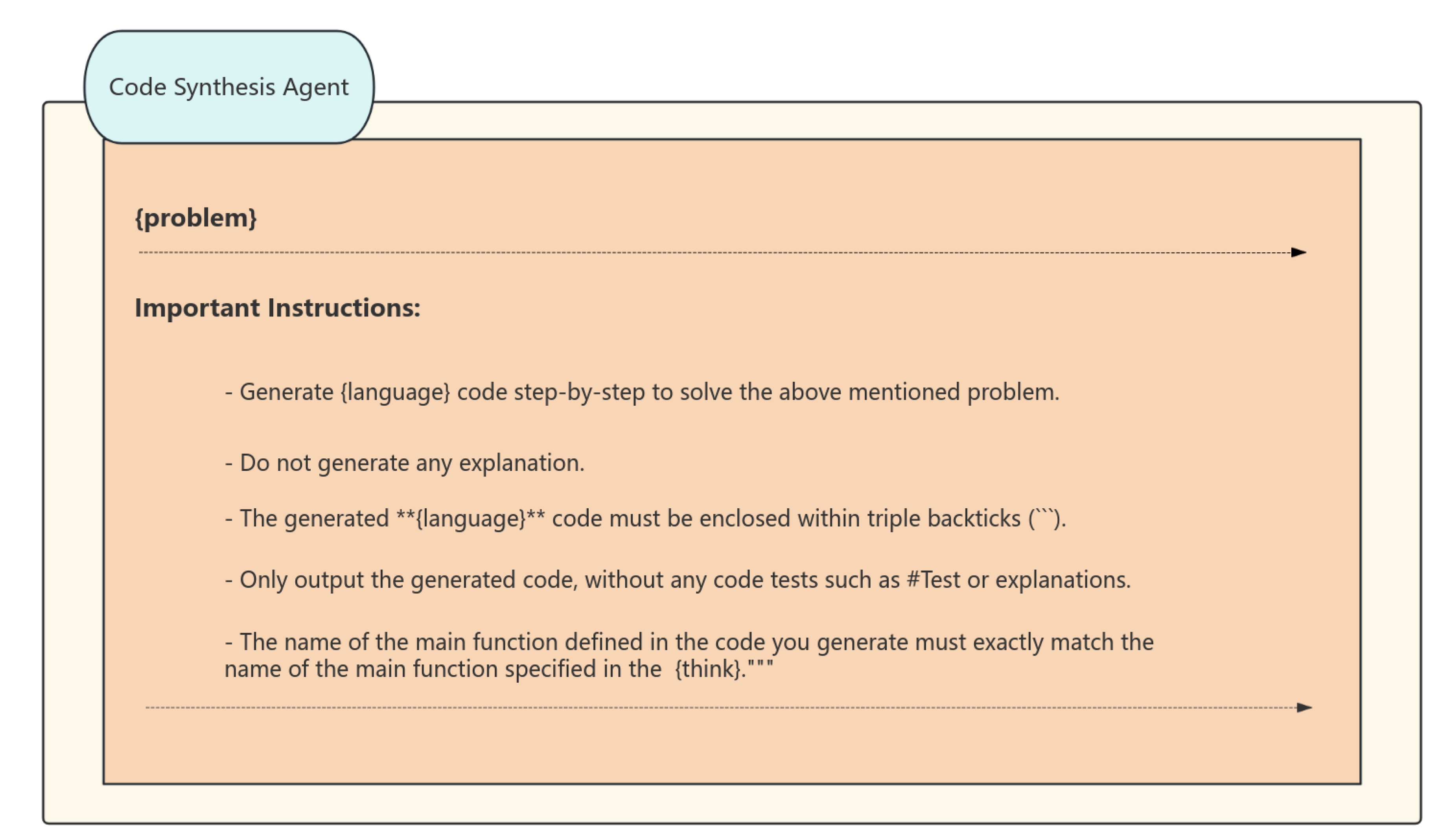
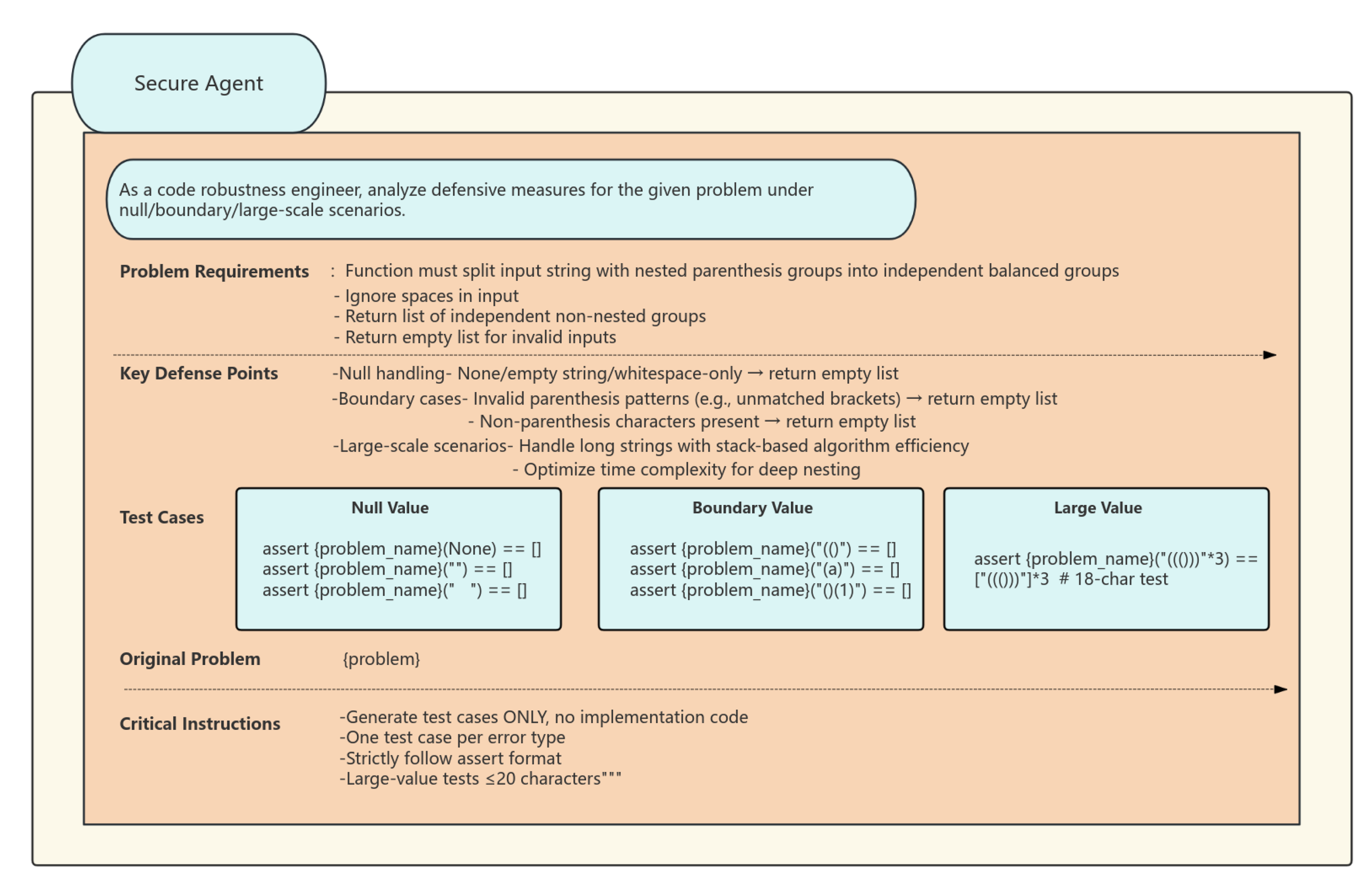
The function of the Code Synthesis Agent is to transform algorithm descriptions into executable code, with its process segmented into three essential phases. Initially, in the constraint-aware generation phase, it utilizes algorithm examples obtained from the Case Retrieval Agent and employs large language models that have undergone instruction fine-tuning to produce foundational code that complies with API standards and syntactical constraints. Subsequently, during the adversarial testing phase, it utilizes a hybrid approach to generate a collection of test cases. It specifically analyzes function signatures to create test cases for boundary situations, such as empty inputs and extreme values, and then extends foundational code templates to build supplementary test cases. Ultimately, at the code expansion phase, it executes syntax-preserving transformations on the underlying code, including loop unrolling and API substitution, producing candidate code with many implementation alternatives,incorporates defensive programming approaches to enhance code robustness. Furthermore, it assesses and enhances the efficacy of the test case suite using mutation testing, systematically eliminating ineffective test cases. For the task of "implementing quicksort," it may generate many code versions, including recursive, iterative, and parallel divide-and-conquer optimizations, while guaranteeing each version includes test cases that account for exceptions in partitioning strategies.

Figure 3. illustrates the Code Synthesis Agent’s code prompt and word image.

Figure 3. illustrates the Code Synthesis Agent’s code prompt and word image.

3.2.3. Defect Diagnosis Agent

The Defect Diagnosis Agent serves as the ultimate safeguard in quality control, employing a hierarchical diagnostic strategy to evaluate and enhance unsuccessful solutions. Initially, it conducts a preliminary diagnosis by examining the logs of failed tests to ascertain the specific test case that failed and to identify the discrepancies between anticipated and actual outputs. Consequently, it does a cursory analysis. It further uses control flow graphs and data dependency analysis to trace the issue to its origin and ascertain the fundamental cause of the code mistake. Ultimately, it provides repair recommendations and establishes a knowledge base of error patterns and repair strategies. It offers systematic remediation recommendations for prevalent faults, including insufficient management of boundary conditions and race condition problems. This intelligent agent is capable of conducting multi-level, multi-granularity analysis and diagnosis, including individual lines of code to comprehensive architectural patterns, while providing practical enhancement strategies. For instance, if it identifies insufficient safeguards against a "hash table collision attack", it will advocate for the use of salt randomization and propose optimal practices for particular encryption libraries.

This module functions through the collaboration of three intelligent agents, establishing a closed-loop optimization via a circular feedback mechanism. The diagnostic agent’s defect analysis results are utilized to enhance the semantic weighting of instance retrieval, while the test cases gathered during code synthesis consistently augment the historical case repository. The recall agent adaptively modifies retrieval preferences according to diagnostic feedback, allowing the system to independently evolve and improve its problem-solving methodology. This design transcends the linear limitations of conventional pipeline layouts, enabling the system to exhibit adaptive characteristics like those observed in biological systems.

Figure 4. Defect Diagnosis Agent Code prompt word image

Figure 4. Defect Diagnosis Agent Code prompt word image

Figure 5. Secure Agent Code prompt word image

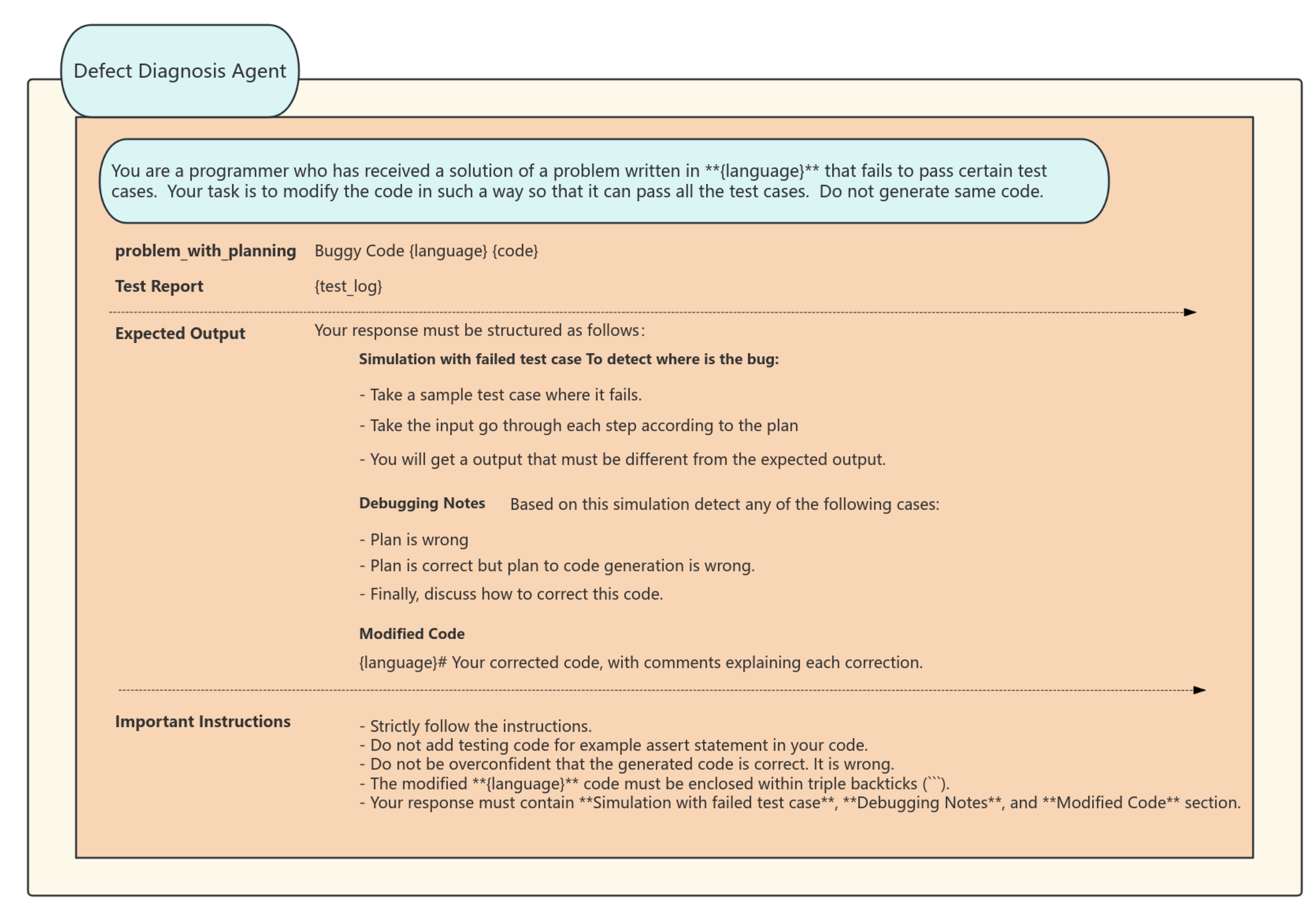
Figure 5. Secure Agent Code prompt word image

3.3. Evolutionary Annealing Optimization Module

3.3.1. Objective of Module Design

The design of the evolutionary annealing optimization module aims to attain equilibrium in dynamic exploration by amalgamating evolutionary and annealing techniques to ascertain the ideal solution. The simulated annealing algorithm is a stochastic optimization technique derived from the concept of solid annealing. It evades local optima by probabilistically accepting suboptimal solutions in its pursuit of the global optimal solution. Nonetheless, this approach possesses a notable limitation: its sluggishness renders it inappropriate for intricate optimization challenges. We employ the evolutionary genetic algorithm to manage optimization jobs. This hybrid methodology integrates the global exploration potential of simulated annealing with the swift convergence of evolutionary algorithms, thereby augmenting optimization efficiency and bolstering the algorithm’s robustness. Consequently, it is better prepared to address intricate and evolving optimization situations.

3.3.2. Core Optimization Procedure

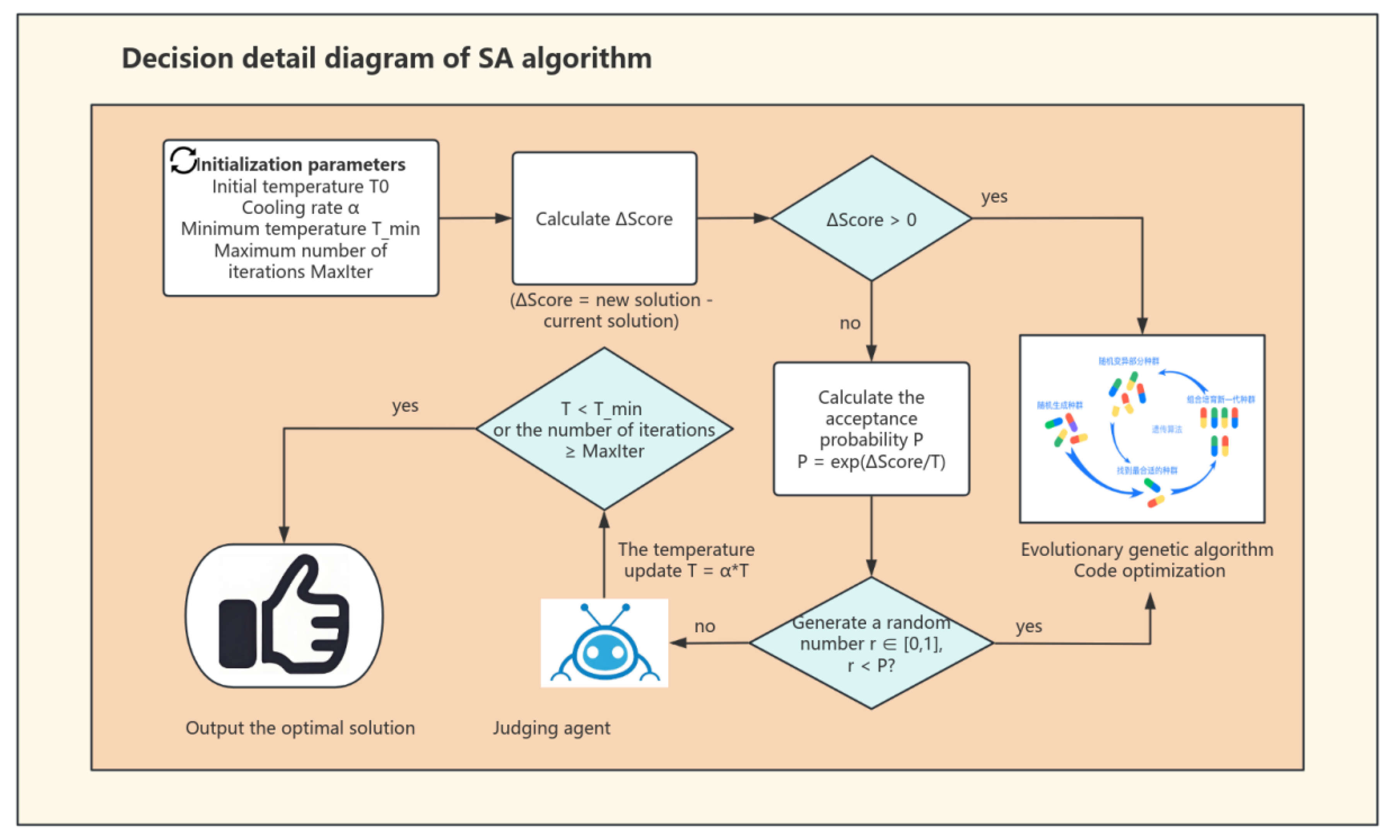
The optimization procedure commences with the appropriate setting of initialization parameters, encompassing initial temperature $T_0$, cooling rate $\alpha$, minimum temperature $T_{\min }$, and maximum iteration count MaxIter. These parameters must be adaptively formulated according to certain conditions. The disparity between the multi-dimensional fitness score of the current candidate solution and that of the previous solution is computed during the generation of new candidate solutions. The annealing-driven choice utilizes this disparity to ascertain whether to accept the new answer. If $\Delta \mathrm{Score}>0$, it signifies that the new solution surpasses the previous one in a thorough assessment across various dimensions. The new solution is approved and advanced to the optimization step of the evolving genetic algorithm. Optimization is executed by selection, crossover, and mutation operations. The optimized solution is subsequently returned to the test validation module for additional annealing determinations until the specified threshold criteria are satisfied. This iterative closed-loop design creates a self-sustaining evolution model for problem-solving. If $\Delta \mathrm{Score}<0$, the new solution is deemed inferior to the previous one in the overall assessment. The acceptance probability of the new solution is dynamically regulated according to the temperature parameter T. Rejected solutions activate the Defect Diagnosis Agent for dynamic feedback, supplying faulty information to modify the optimization trajectory. This feedback is transmitted to the case backtracking intelligent agent to produce new algorithmic solutions. This approach guarantees that the optimization process can thoroughly investigate the solution space while circumventing entrapment in local optimum solutions.

Figure 6. Detailed Diagram of Simulated Annealing Decision Process.

Figure 6. Detailed Diagram of Simulated Annealing Decision Process.

3.3.3. Innovation Mechanism

In the annealing decision module, the acceptance probability of suboptimal solutions is governed by the temperature T. We utilize a dynamic adjustment technique for temperature T. The initial temperature $T_0$ is established according to the problem’s complexity. $T_0$ is defined by the quantity of initial candidate solutions and their respective fitness ratings. If the average fitness decreases, indicating a more challenging problem, we will increase the temperature to extend the exploration phase. The adaptive technique, unlike a constant temperature such as $T_0$ set at 1000, facilitates expedited convergence and reduces computing expenses in simpler tasks while ensuring sufficient exploration in difficult tasks, enhancing convergence speed by 30% in datasets like APPS.

$$T_0={\displaystyle \frac{N·(f_{max}-\overline{f})}{\sqrt{{\sigma }_f^2+ϵ}}}$$

(1)

$f_{max}$:the maximum value of fitness theory (such as the upper limit of scoring). $\overline{f}$:the average fitness score of the initial population. ${\sigma }_f^2$:initial fitness variance. $ϵ$:smoothing factor (to prevent the denominator from being 0, usually taking the value of $ϵ=1$) . The formula dynamically sets the initial temperature to suit the problem’s complexity. It ensures that harder problems, which usually have a lower average fitness in the initial population, get a higher T0. This allows for broader exploration of the solution space. By doing so, it helps the algorithm avoid getting trapped in local optima early on and significantly improves the efficiency of the optimization process.

We employ an adaptive dynamic cooling adjustment method that integrates exponential cooling with variance feedback to mitigate temperature fluctuations. The present population fitness variance (${\sigma }_{\mathrm{fit}}^2$) indicates the diversity of solutions. An elevated value signifies more population diversity and a wider range of solutions, necessitating a reduced cooling rate to extend the exploration phase. Conversely, less variance in population fitness indicates an increasing homogeneity within the population, requiring expedited cooling for swifter convergence. The constant C functions as a tuning parameter to regulate the sensitivity of the cooling rate to variability. According to previous study experience, C is often established at 100 to equilibrate the effects of variance variations.

$$T_{k+1}=\alpha ·T_k·exp\left(-{\displaystyle \frac{{\sigma }_{\mathrm{fit}}^2}{C}}\right)$$

(2)

$T_{k+1}$: The temperature of the next generation, controlling the degree of attenuation of the acceptance probability of the inferior solution. $T_k$: The current temperature affects the exploration ability of the current iteration. $\alpha$:The basic cooling coefficient is the reference rate of temperature attenuation that determines the temperature. ${\sigma }_{\mathrm{fit}}^2$:Population fitness variance measures the diversity of the current solution. C:Variance sensitivity adjustment constant, controlling the influence of variance on the cooling rate. This formula adjusts cooling based on solution diversity: slows cooling to explore when diverse, speeds up when converging.

The dynamic temperature adjustment approach proficiently addresses the limitations of conventional exponential cooling, which employs a constant cooling rate, such as $\alpha =0.95$. This conventional method fails to ascertain the true condition of the population, which may result in premature convergence or superfluous iterations. Conversely, the hybrid strategy regulates temperature adaptively, enabling a reduction that responds dynamically to the problem’s complexity. When addressing issues of greater complexity or significant initial variance, this strategy automatically prolongs the high-temperature phase. It attains rapid convergence for less complex problems.

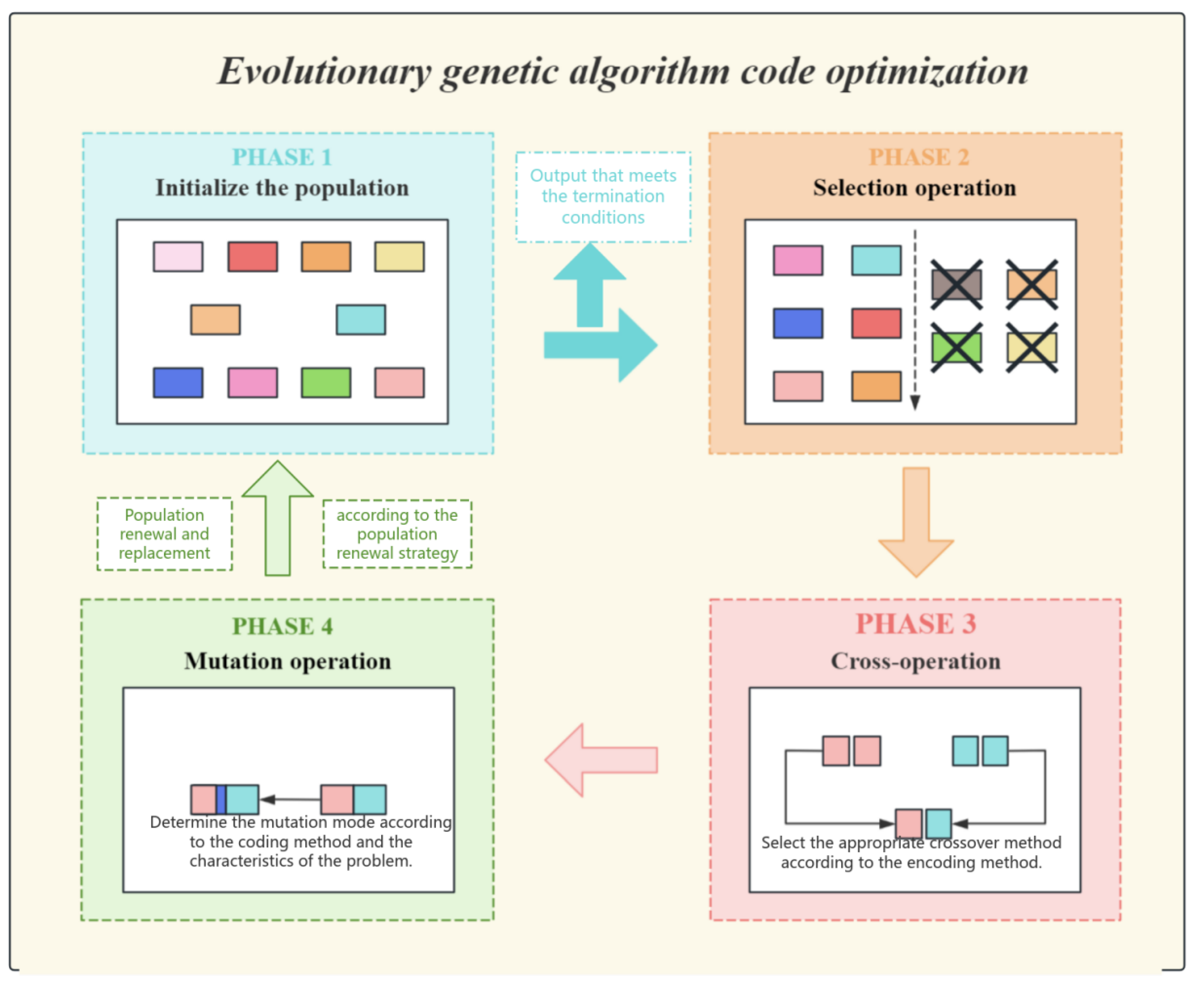
Figure 7. The Detailed Diagram of Evolutionary Genetic Optimization.

Figure 7. The Detailed Diagram of Evolutionary Genetic Optimization.

The fundamental decision-making mechanism of simulated annealing relies on the probability acceptance criterion dictated by temperature T. This criterion is the principal mechanism for determining the acceptance of a suboptimal solution—a new solution with a score inferior to the existing one. $\Delta \mathrm{Score}$ is defined as Scorenew minus Scorecurrent, indicating the score disparity between the new and current solutions, and T denotes the current temperature parameter. When $\Delta \mathrm{Score}$ exceeds 0, it signifies that the new answer is superior and will be accepted unequivocally. Nevertheless, when $\Delta \mathrm{Score}$ is less than or equal to zero, the new solution is deemed suboptimal. However, even if the new approach reduces the readability of the code while presenting an innovative structure, there is a certain likelihood of its preservation. The retention likelihood is predominantly influenced by temperature T. In the high-temperature phase, the algorithm is inclined to accept suboptimal solutions, promoting the exploration of novel regions, particularly in the initial phases. By doing comprehensive searches throughout the solution space, it prevents entrapment in local optima. In the low-temperature phase, the algorithm prioritizes fine-tuning in its later phases, concentrating on high-quality solutions while nearly discarding all inferior options and prioritizing localized optimization.

$$P\left(\Delta \mathrm{Score}\right)=exp\left(-{\displaystyle \frac{\Delta \mathrm{Score}}{T}}\right)$$

(3)

$P_{accept}$: The probability of acceptance of the inferior solution. $\Delta$Score: The difference in fitness between the new solution and the current solution. T: Current temperature. At high T, it accepts some worse solutions to escape local optima; at low T, becomes increasingly greedy.

Convergence determination formula provides a clear stopping condition for the algorithm. It halts iterations when the maximum adaptation change in the last five iterations falls below a predefined threshold, indicating that the algorithm has reached a stable state. This ensures that computational resources are used efficiently, preventing unnecessary iterations once the solution has stabilized and saving time and computational power for more productive use.

$$\mathrm{Convergence}\mathrm{mark}=\left\{\begin{array}{cc}1\hfill & max\left(\Delta Scor{e}_{\mathrm{last}5}\right)<ϵ\hfill \\ 0\hfill & \mathrm{therwise}\hfill \end{array}\right.$$

(4)

$\Delta Score$:the score changes in the last five iterations. $ϵ=0.01$:convergence threshold,termination when the score fluctuation is less than 1%. This formula flags convergence if score improvements are less than 1% over five generations.

The resource consumption constraint formula acts as a financial advisor for the algorithm, meticulously setting a token budget to keep resource usage in check. It plays the role of a vigilant supervisor, continuously monitoring how many tokens the algorithm is gobbling up during its operations. If the algorithm starts to overspend and exceeds the predefined budget, the formula steps in like a strict accountant, terminating further iterations to prevent any wasteful resource drain. This makes the algorithm a perfect fit for those tight-budget, resource-constrained environments where computational resources are as precious as gold, and every ounce of efficiency counts towards making the algorithm’s practical implementation a reality.

$$\mathrm{Token}\mathrm{budget}=\sum _{k=1}^K(N_k·\mathrm{TokenCost})\le B_{max}$$

(5)

$N_k$:the number of candidate solutions generated in the KTH iteration. TokenCost:token consumption of a single candidate solution. $B_{max}$: Maximum token budget. Enforces token/API call limits by reducing population size or early stopping when approaching budget.

In a multi-dimensional scoring system, fitness scores are assessed based on four indicators. Functional correctness is assessed by test case pass rates; execution efficiency is shown by normalized scores of time and memory utilization; symmetry encompasses logical branch symmetry and interface symmetry; and readability is evaluated based on static analysis scores from Pylint. Concerning dynamic weight regulations, if the problem description includes terms like "efficient" or "low latency," $w_2$ is elevated to $0.5$. In the event that symmetry constraints are identified, $w_3$ is established at a minimum of 0.3. Customized scoring criteria are established based on particular specifications, producing solutions that more closely conform to the intended standards.

$$Fitness\left(t\right)=\sum _{i=1}^4{w}_i\left(t\right)·f_i$$

(6)

$w_i$:the weight $w_i$ is dynamically adjusted. fi:The fitness score of the i-th dimension. Weighted combination of functionality, efficiency, symmetry , and readability , with dynamic adjustments.

Table 2. The weight of each scoring dimension can be dynamically adjusted according to actual needs to reflect its importance in the overall scoring. For example, if the time complexity is particularly important in the scenario, a higher weight can be set for it

Code set	Time complexity	Space complexity	Code readability	Test pass rate	Final score
Evaluation Code 1		×		80%	75
Evaluation Code 2	×			90%	78
Evaluation Code 3			×	85%	85

Table 2. The weight of each scoring dimension can be dynamically adjusted according to actual needs to reflect its importance in the overall scoring. For example, if the time complexity is particularly important in the scenario, a higher weight can be set for it

Code set	Time complexity	Space complexity	Code readability	Test pass rate	Final score
Evaluation Code 1		×		80%	75
Evaluation Code 2	×			90%	78
Evaluation Code 3			×	85%	85

The essential component of the evolutionary operation is the evolving genetic algorithm, which employs a hybrid approach between elitism and tournament selection during the selection phase. Only individuals in the top ten percent of fitness are directly kept for the subsequent generation, while the remaining individuals produce parents via tournament selection. The crossover operation can be incorporated with the defensive code template library, encompassing input validation, error handling, and boundary condition checks, thereby ensuring that the resulting code operates correctly and adheres to robust defensive programming principles. We employ directed syntax mutation to enhance code robustness, which has proven to be more effective than random mutation techniques. Utilizing boundary reinforcement, dynamic boundary verifications are incorporated within loops or conditional expressions.

$$P_{\mathrm{select}}={\displaystyle \frac{f_i}{{\sum }_{j\in \mathrm{tournament}}{f}_j}}$$

(7)

$f_i$: individual fitness. This formula is essentially a dynamic balance point established between "ensuring the convergence quality" and "maintaining the exploration ability", and its parameters (10% elite ratio, tournament size 5) have been determined through empirical research as the optimal configuration for the code generation task.

The defensive cross-operation formula is like a clever safeguard woven right into the fabric of the code-generation crossover process. It’s not just about mixing and matching code snippets; it’s about embedding smart defensive programming techniques. By weaving in error-handling mechanisms that act like safety nets, catching and managing any unexpected hiccups, along with input validation that acts as a strict gatekeeper, ensuring only the right kind of data gets through, and boundary condition checks that keep a vigilant eye on the code’s operational limits, this formula gives the generated code a real boost in terms of robustness and reliability. This means fewer nasty runtime errors and exceptions popping up to ruin the party, and code that doesn’t just do its job right but also stands strong against all sorts of error-inducing challenges. All in all, it’s a big win for the overall quality and maintainability of the software, making it a breeze to keep in tip-top shape for the long haul.

$$\mathrm{Offspring}\mathrm{code}={\Phi }_{\mathrm{cross}}({\mathrm{Parent}}_1,{\mathrm{Parent}}_2)\cup \mathrm{DefenseTemplate}$$

(8)

${\Phi }_{\mathrm{cross}}$:standard crossover operations, such as single-point crossover or uniform crossover. DefenseTemplate:a defensive code template library, including modules such as input validation and error handling. This formula flexibly combines the parent solution with the forcibly injected defense template (input validation, error handling) to enhance the defense performance of the generated code.

Directional grammar variation formula identifies vulnerable points in the code structure for mutation. By analyzing the code’s syntax and pinpointing areas that are prone to errors or have weak error-handling capabilities, it applies targeted mutations. This approach aims to optimize code quality and robustness, ensuring that the generated code can gracefully handle edge cases and exceptions, thereby improving its reliability and reducing the need for extensive post-generation debugging.

$$\mathrm{Variant}\mathrm{position}=arg\underset{s\in \mathrm{AST}}{max}\left({\displaystyle \frac{\partial \mathrm{Score}}{\partial s}}\right)$$

(9)

AST:the tree-like structure representation of the code. ${\displaystyle \frac{\partial \mathrm{Score}}{\partial s}}$:the sensitivity of fitness score to code node s. We can use formulas to locate sensitive nodes through AST analysis, for example, automatically insert range validation logic above loop statements.

The formula for population diversity is designed to maintain a healthy balance within the genetic algorithm by monitoring the diversity of solutions. When diversity is too low, it indicates that the population may be converging prematurely on a suboptimal solution. Conversely, when diversity is too high, it may suggest that the algorithm is not effectively focusing on the most promising solutions. By tracking these levels, the formula ensures the algorithm doesn’t settle for suboptimal results too quickly and continues to explore the solution space effectively.This balance is crucial as it prevents the algorithm from becoming trapped in local optima, instead encouraging a thorough exploration that can lead to the discovery of high-quality solutions which might otherwise be missed. The benefits of this mechanism are significant, as it enhances the algorithm’s ability to find more optimal solutions, improves the overall efficiency of the optimization process, and increases the likelihood of achieving better results in a wide range of applications. By maintaining this balance, the genetic algorithm can operate at its best, delivering more reliable and effective solutions to complex problems.

$$\mathrm{Diversity}={\displaystyle \frac{{\sigma }_{\mathrm{fit}}^2}{{\overline{f}}^2}}\times 100\%$$

(10)

${\sigma }_{\mathrm{fit}}^2$:population fitness variance. $\overline{f}$:population average fitness.The population diversity metric quantifies solution spread by normalizing fitness variance against mean fitness. It dynamically regulates exploration: triggers forced mutation when diversity drops below 5% (preventing premature convergence) and restricts crossover above 20% (controlling excessive randomness). This maintains optimal genetic variation throughout evolution.

4. Experimental Configuration

4.1. Dataset

To comprehensively evaluate the performance of our model on general programming problems, we have selected the following four representative programming datasets: HumanEval [32], HumanEval-ET [32], EvalPlus and MBPP. The MBPP dataset we’ve curated consists of 397 carefully selected problems from an initial pool of over 1,000 candidates, representing the most practical programming challenges across file operations, API calls, and data processing tasks. These problems mirror real-world development scenarios—like "reading a CSV file and calculating the average of a specific column"—and incorporate common engineering challenges such as robust exception handling.

Figure 8. The Detailed Diagram of Evolutionary Genetic Optimization.

Figure 8. The Detailed Diagram of Evolutionary Genetic Optimization.

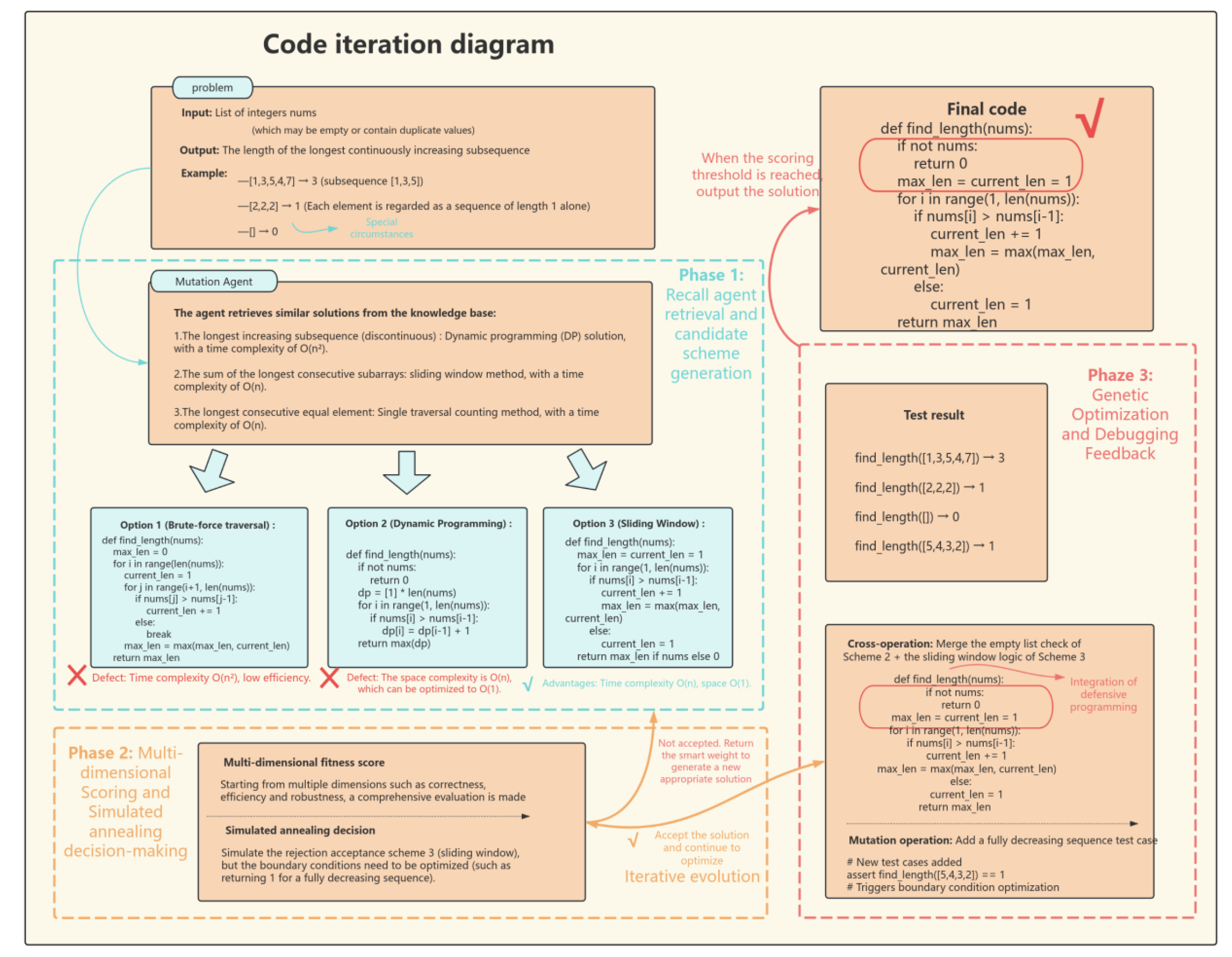
Table 3. Dataset Statistics and Characteristics

Dataset Name	Number of Problems	Programming Language	Problem Type
HumanEval	164 Problems	Python	Functional Correctness, verified by unit tests to ensure generated code solves the problem correctly
HumanEval-ET	164 Problems	Python	The extended test version of HumanEval, proposed by the academic community, aims to enhance the robustness evaluation capability of the original dataset
EvalPlus	164 Problems	Python	Integrate multiple datasets (such as HumanEval, MBPP) and enhance the testing intensity
MBPP	397 Problems	Python	It covers practical tasks such as file operations, API calls, and data processing

Table 3. Dataset Statistics and Characteristics

Dataset Name	Number of Problems	Programming Language	Problem Type
HumanEval	164 Problems	Python	Functional Correctness, verified by unit tests to ensure generated code solves the problem correctly
HumanEval-ET	164 Problems	Python	The extended test version of HumanEval, proposed by the academic community, aims to enhance the robustness evaluation capability of the original dataset
EvalPlus	164 Problems	Python	Integrate multiple datasets (such as HumanEval, MBPP) and enhance the testing intensity
MBPP	397 Problems	Python	It covers practical tasks such as file operations, API calls, and data processing

4.2. Baseline and Indicators

To thoroughly assess AnnCoder’s performance, we chose multiple representative baseline approaches. Direct prompting instructs the language model to produce code autonomously, depending solely on the proficiency of large language models. Chain-of-thought prompting [33] disaggregates the problem into sequential solutions to proficiently address intricate problems. Self-Planning [29] delineates the code generation process into planning and implementation phases. Reflexion [5] offers feedback derived from unit test outcomes to improve solutions. AlphaCodium systematically refines code with AI-generated input-output assessments. CodeSIM is a multi-agent framework for code generation that mimics the complete software development lifecycle to enhance the efficiency and quality of code production. MapCoder integrates three categories of LLM prompts—retrieval, planning, debugging, and code generation—effectively emulating the complete program synthesis cycle exhibited by human coders. To ensure a fair comparison, our assessment employed OpenAI’s ChatGPT and GPT-4. The evaluation criteria utilized is the commonly accepted pass@1 measure, which considers the model successful if its sole projected solution is accurate.

Table 4. Performance Comparison.

LLM	Approach	HumanEval	HumanEval-ET	EvalPlus	MBPP
ChatGPT	Direct	71.3%	64.6%	67.1%	75.8%
	CoT	70.7%	63.4%	68.3%	78.3%
	Self-Planning	70.7%	61.0%	62.8%	73.8%
	Self-collaboration	74.4%	56.1%	-	68.2%
	CodeSim	86.0%	72.0%	73.2%	86.4%
	MapCoder	80.5%	70.1%	71.3%	78.3%
	Anncoder	86.6%	73.2%	78.0%	85.9%
		↑6.1%	↑3.1%	↑6.7%	↑7.6%
GPT4	Direct	80.1%	73.8%	81.7%	81.1%
	CoT	89.0%	61.6%	-	82.4%
	Self-Planning	85.4%	62.2%	-	75.8%
	Reflexion	91.0%	78.7%	81.7%	78.3%
	CodeSim	94.5%	81.7%	84.8%	89.7%
	MapCoder	93.9%	82.9%	83.5%	83.1%
	Anncoder	90.9%	85.4%	84.8%	90.7%
		↓3.0%	↑2.5%	↑1.3%	↑7.6%

Table 4. Performance Comparison.

LLM	Approach	HumanEval	HumanEval-ET	EvalPlus	MBPP
ChatGPT	Direct	71.3%	64.6%	67.1%	75.8%
	CoT	70.7%	63.4%	68.3%	78.3%
	Self-Planning	70.7%	61.0%	62.8%	73.8%
	Self-collaboration	74.4%	56.1%	-	68.2%
	CodeSim	86.0%	72.0%	73.2%	86.4%
	MapCoder	80.5%	70.1%	71.3%	78.3%
	Anncoder	86.6%	73.2%	78.0%	85.9%
		↑6.1%	↑3.1%	↑6.7%	↑7.6%
GPT4	Direct	80.1%	73.8%	81.7%	81.1%
	CoT	89.0%	61.6%	-	82.4%
	Self-Planning	85.4%	62.2%	-	75.8%
	Reflexion	91.0%	78.7%	81.7%	78.3%
	CodeSim	94.5%	81.7%	84.8%	89.7%
	MapCoder	93.9%	82.9%	83.5%	83.1%
	Anncoder	90.9%	85.4%	84.8%	90.7%
		↓3.0%	↑2.5%	↑1.3%	↑7.6%

5. Result

5.1. Fundamental Code Generation

The baseline data used in this study is derived from the work of [34] . Specifically, we utilize the performance metrics reported in their paper as our baseline for comparison. This includes the accuracy obtained by their model on the same dataset. The selection of this baseline is motivated by its relevance to our research problem and its widespread use in the field, providing a fair and meaningful comparison to evaluate the effectiveness of our proposed model.

Comparative trials with multiple baseline approaches reveal that Anncoder has superior performance in all benchmark tests, significantly outperforming all baseline methods. In fundamental programming tasks such as HumanEval and MBPP, AnnCoder exhibits significant performance improvements, attaining90.9% and 90.7%, respectively. These findings clearly demonstrate AnnCoder’s supremacy in code generation tasks, indicating enhancements in various aspects, including correctness, efficiency, and readability. Through the employment of multi-agent collaboration, multi-objective optimization, and dynamic feedback mechanisms, Anncoder proficiently addresses the shortcomings of current technologies regarding practicality and robustness.

5.2. Cross-open-source LLMs performance

Our analysis of AnnCoder’s performance across different LLMs reveals important architectural strengths and limitations. GPT-4.0 shows clear advantages in complex algorithmic tasks, outperforming ChatGPT by 12.2% on challenging HumanEval-ET where its superior handling of edge cases and defensive coding shines. However, this lead narrows to just 4.8% on practical MBPP engineering tasks, suggesting GPT-4.0’s sophisticated approach can sometimes overcomplicate solutions. The model maintains a consistent 6.8% overall advantage in comprehensive evaluations, particularly excelling at code standardization while showing room for improvement in exception handling. These findings highlight how task requirements should guide model selection - GPT-4.0 excels at deep algorithmic work but may benefit from constraints when applied to more straightforward engineering problems. The results point to the value of developing adaptive systems that can leverage each architecture’s strengths while compensating for their weaknesses.

Table 5. A comparison of AnnCoder’s performance on cross-open-source LLMs.

Dataset	ChatGPT	GPT-4.0	Performance Change
HumanEval	86.6%	90.9%	+4.3%
HumanEval-ET	73.2%	85.4%	+12.2%
MBPP	85.9%	90.7%	+4.8%
EvalPlus	78.0%	84.8%	+6.8%

Table 5. A comparison of AnnCoder’s performance on cross-open-source LLMs.

Dataset	ChatGPT	GPT-4.0	Performance Change
HumanEval	86.6%	90.9%	+4.3%
HumanEval-ET	73.2%	85.4%	+12.2%
MBPP	85.9%	90.7%	+4.8%
EvalPlus	78.0%	84.8%	+6.8%

6. Ablation Research and Analysis

6.1. Module Validity Verification

6.1.1. Verification Method

The model’s performance was evaluated following the removal of particular modules to assess the efficacy of the three fundamental components of Anncoder: genetic optimization, simulated annealing, and the defensive template library. We created three control groups, each excluding one of the following components: genetic optimization, simulated annealing decision-making, or the defensive template library. Table has details.Experiments were performed on the specified dataset-HumanEval, encompassing intricate scenarios such as null inputs, extreme values, and boundary conditions, including problems such as array out-of-bounds errors and vast number overflows. We employed multi-dimensional assessment metrics to conduct a comparative analysis of the contributions of the core components.

Table 6. Settings of the control group.

Dataset Name	Module Removal	Replacement Strategy
Anncoder-NoGA	Genetic Algorithm (Crossover/Mutation)	Random Search: Randomly generate code variants
Anncoder-NoSA	Simulated Annealing Decision	Greedy Strategy: Only accept better solutions
Anncoder-NoDefense	Defensive Template Library	Disable templates, only generate basic logic code

Table 6. Settings of the control group.

Dataset Name	Module Removal	Replacement Strategy
Anncoder-NoGA	Genetic Algorithm (Crossover/Mutation)	Random Search: Randomly generate code variants
Anncoder-NoSA	Simulated Annealing Decision	Greedy Strategy: Only accept better solutions
Anncoder-NoDefense	Defensive Template Library	Disable templates, only generate basic logic code

Figure 9. Module validity verification:Remove the genetic optimization, simulated annealing decision-making and defensive template libraries respectively.

Figure 9. Module validity verification:Remove the genetic optimization, simulated annealing decision-making and defensive template libraries respectively.

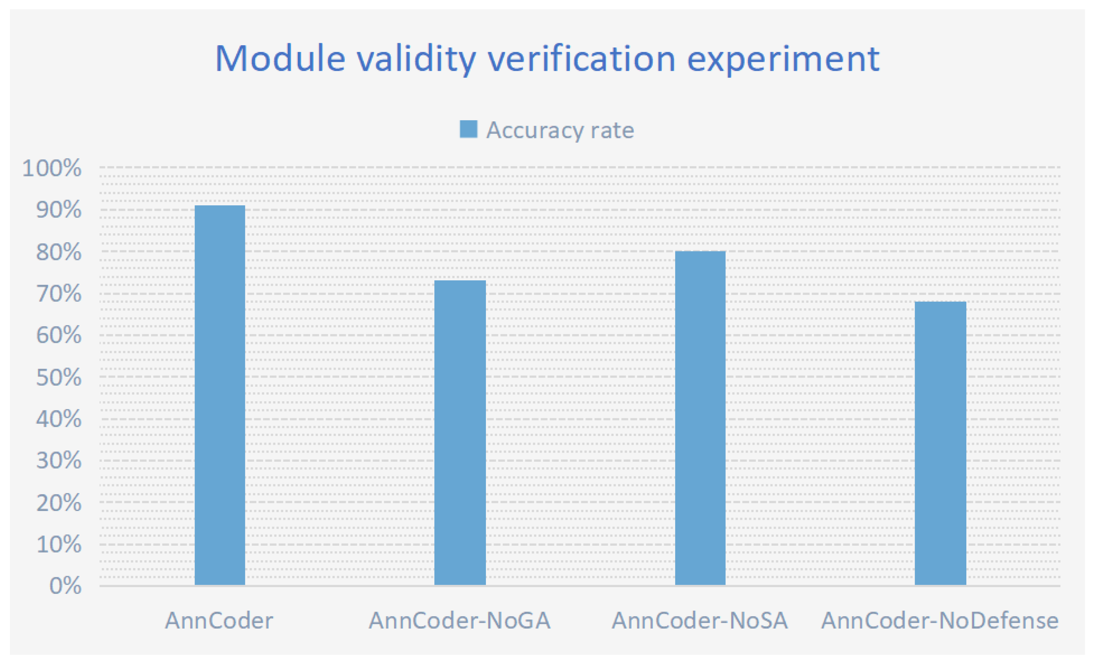
Table 7. Data and Results.

Model	Accuracy Rate
Anncoder	91%
Anncoder-NoGA	73%
Anncoder-NoSA	80%
Anncoder-NoDefense	68%

Table 7. Data and Results.

Model	Accuracy Rate
Anncoder	91%
Anncoder-NoGA	73%
Anncoder-NoSA	80%
Anncoder-NoDefense	68%

6.1.2. Analysis of Results

The study of the trial findings indicated that the lack of the genetic optimization module resulted in an 18% reduction in the model’s overall accuracy. The typical random search strategy was ineffective at amalgamating beneficial codes from parent generations, such as defensive logic, during the initial generation phase. Such a scenario may lead to overlooked validations for empty lists and analogous problems, ultimately resulting in increased failures during the initial generation. The elimination of the genetic optimization module resulted in a heightened frequency of repairs, as dependence on random search demanded increased attempts to sporadically produce correct logic, exemplified by employing five random mutations to integrate math.ceil. Utilizing a structured code evolution strategy can expedite problem identification, improve accuracy, and reduce the number of necessary corrections.

Upon the removal of the simulated annealing (SA) module, the model’s accuracy decreased by 11%. The decision control mechanism of simulated annealing is essential, as it probabilistically accepts poor solutions to prevent entrapment in a local optimum caused by greedy selection. An erroneous preference for round() instead of ceil() may arise; nevertheless, the annealing mechanism allows for the provisional acceptance of subpar solutions to investigate the global optimum and prevent early convergence to substandard defense logic. A prominent instance is observed in the test input [1.4, 4.2, 0], where the SA-driven model transitioned from round() math.ceil(), but a greedy strategy was unable to enable this alternative approach.

Disabling the defensive template library resulted in the model’s inability to provide null-checking code, such as if not nums: return 0, or large-number truncation code like min(total, 2^32 - 1), causing a significant 23% decrease in accuracy. Deactivating the template library may lead to unaddressed edge cases, such as null inputs, which can directly precipitate runtime issues. An experimental study indicates that, out of 50 medium-difficulty issues on LeetCode, failures in 32 questions were due to a lack of defensive coding practices.

6.2. Sensitivity Analysis of Hyperparameters

6.2.1. Objective of Sensitivity Analysis

Anncoder includes three hyperparameters: the fundamental parameters of the genetic algorithm, specifically the number of iterations, Variance, and the annealing strategy. The study examines the effects of Variance, number of iterations and annealing strategy on model performance, focusing on achieving an optimal balance between accuracy and convergence speed. In real applications, parameter combinations can be deliberately chosen to meet different scenario requirements, emphasizing either high precision or minimal resource use.

6.2.2. Experimental Design

We selected three values of convergence steps, three variances and two annealing strategies , resulting in a total of 18 combinations. Experiments were conducted on the dataset -HumanEval. The problems included dynamic programming, array operations and graph algorithms to ensure a balanced range of complexity.

Every combo was executed five times. The evaluation measures comprised overall accuracy, convergence steps (the mean number of iterations from the starting code to the final correct version), and stability (quantified by the standard deviation of five independent experiments) to evaluate parameter sensitivity. Simultaneously, the defensive template library and the initial population size were kept constants to avoid interfering with the effects of the parameters. ANOVA was employed for statistical testing to evaluate the primary impacts of parameters, and Tukey HSD was utilized for post-hoc analysis.

Table 8. Parameter Settings and Design Rationale.

Parameter	Value Range	Design Rationale
Number of iterations	2, 3, 4	Fewer iterations are used for rapid convergence of simple tasks, while more iterations are used for fully exploring the solution space of complex tasks.
Variance	1, 3, 5	A lower variance maintains stability and avoids noise interference. A higher number of variations enhances population diversity and avoids premature convergence.
Annealing strategy	Group 1: At 1000℃, an extension score of 0.3 is allowed to pass; at 500℃, 0.6 is allowed to pass; at 0℃, 0.8 is allowed to pass. <br> Group 2 The basic score at 1000℃ is 1 to pass, at 500℃ it is 0.6 to pass, at 0℃ it is [1,0.8,0.8,0.8] to pass, and at -500℃ it is [1.0, 0.2, 0.2, 0.2] to pass	The first group of strategies involves extensive exploration in the early stage and strict screening in the later stage. The second group of strategies dynamically adjusts the acceptance criteria and lowers the requirements later to avoid optimization stagnation due to problems with test examples.

Table 8. Parameter Settings and Design Rationale.

Parameter	Value Range	Design Rationale
Number of iterations	2, 3, 4	Fewer iterations are used for rapid convergence of simple tasks, while more iterations are used for fully exploring the solution space of complex tasks.
Variance	1, 3, 5	A lower variance maintains stability and avoids noise interference. A higher number of variations enhances population diversity and avoids premature convergence.
Annealing strategy	Group 1: At 1000℃, an extension score of 0.3 is allowed to pass; at 500℃, 0.6 is allowed to pass; at 0℃, 0.8 is allowed to pass. <br> Group 2 The basic score at 1000℃ is 1 to pass, at 500℃ it is 0.6 to pass, at 0℃ it is [1,0.8,0.8,0.8] to pass, and at -500℃ it is [1.0, 0.2, 0.2, 0.2] to pass	The first group of strategies involves extensive exploration in the early stage and strict screening in the later stage. The second group of strategies dynamically adjusts the acceptance criteria and lowers the requirements later to avoid optimization stagnation due to problems with test examples.

6.2.3. Data and Result Analysis

In optimization, the number of iterations, variance, and annealing strategy are key parameters. A high variance can add too much noise, hindering model convergence and reducing performance. When variance is set to 3, it strikes a good balance by increasing population diversity and helping the model escape local optima, while still maintaining stability and improving accuracy and stability.Regarding the number of iterations, too few may be insufficient for complex tasks, while too many can lead to overfitting or local optima. It’s essential to choose an appropriate number based on the task’s complexity.There are two main annealing strategies. The first allows for more initial exploration and later strict solution filtering, which helps in finding high-quality solutions but may discard some promising solutions early on. The second strategy starts with strict quality control and dynamically adjusts the acceptance criteria. At the late stage, it lowers the requirements to avoid optimization stagnation due to inadequate test cases, showing better adaptability for complex problems.

Under normal circumstances, it’s recommended to use the default settings: 4 iterations, variance of 3, and the second annealing strategy. This balances accuracy and efficiency. However, parameters can be dynamically adjusted based on specific problems. For algorithmic logic problems, a higher variance can be used. For input parsing tasks, fewer iterations are suggested.

Figure 10. Key parameter combination performance comparison analysis: It comprehensively presents the comparison of algorithm performance among different parameter combinations .

Figure 10. Key parameter combination performance comparison analysis: It comprehensively presents the comparison of algorithm performance among different parameter combinations .

Figure 11. Parameter combination stability radar chart.

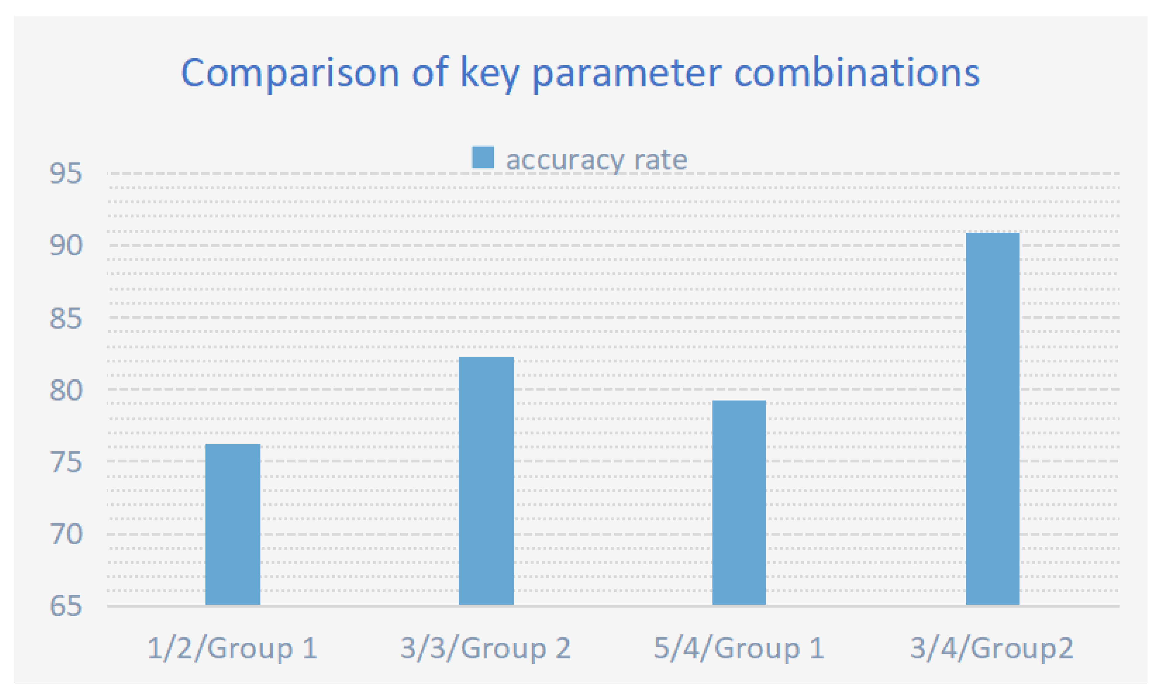
Figure 11. Parameter combination stability radar chart.

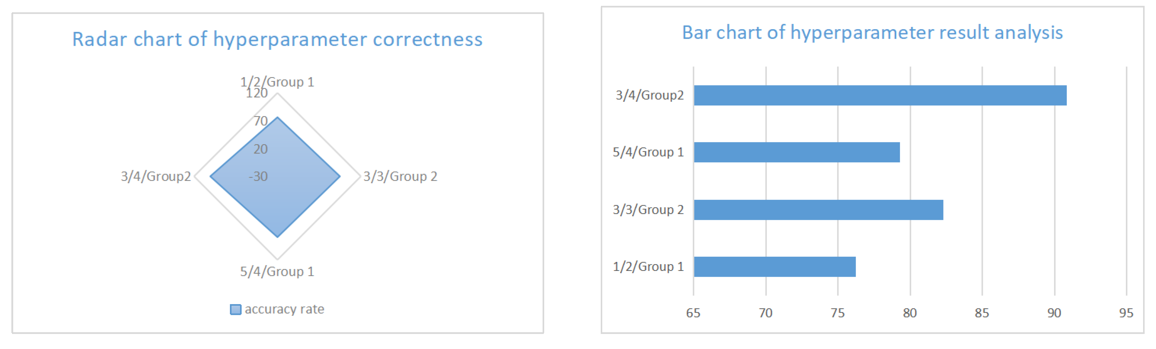
Table 9. Performance Comparison of Parameter Combinations

Parameter Combinations	Accuracy (%)
1/2/Group 1	76.21
3/3/Group 2	82.31
5/4/Group 1	79.27
Best Combination (3/4/Group 2)	90.85

Table 9. Performance Comparison of Parameter Combinations

Parameter Combinations	Accuracy (%)
1/2/Group 1	76.21
3/3/Group 2	82.31
5/4/Group 1	79.27
Best Combination (3/4/Group 2)	90.85

7. Conclusions

This work presents AnnCoder, a novel multi-agent collaboration model engineered to enhance code-generating tasks. It adeptly combines genetic algorithms with simulated annealing techniques, markedly enhancing the precision of code production. We evaluated AnnCoder on many basic datasets and demanding programming datasets. The results indicate its superior performance and potential for effective implementation in contexts such as automated testing and code quality assessment, significantly lowering the expenses associated with human debugging. In resource-constrained contexts, AnnCoder’s efficiency is invaluable, providing a pragmatic code generation solution for devices with restricted computational capabilities. In the future, we will concentrate on adaptive parameter optimization, possibly integrating the Bayesian search algorithm—a robust global optimization method that dynamically modifies crossover and mutation rates according to problem complexity—to maximize Anncoder’s capabilities. These improvements are anticipated to enable AnnCoder to respond more intelligently to a range of programming challenges, from basic scripts to intricate system development. We assert that with continuous improvements in parameter optimization, AnnCoder will play an increasingly crucial role in automated software development, allowing developers to generate superior code at reduced costs and enhanced efficiency.

References

- Paczuski, M.; Bassler, K.E.; Corral, Á. Self-organized networks of competing boolean agents. Physical Review Letters 2000, 84, 3185. [Google Scholar] [CrossRef] [PubMed]
- Valmeekam, K.; Marquez, M.; Sreedharan, S.; Kambhampati, S. On the planning abilities of large language models-a critical investigation. Advances in Neural Information Processing Systems 2023, 36, 75993–76005. [Google Scholar]
- Li, J.; Li, G.; Li, Y.; Jin, Z. Structured chain-of-thought prompting for code generation. ACM Transactions on Software Engineering and Methodology 2025, 34, 1–23. [Google Scholar] [CrossRef]
- Kale, U.; Yuan, J.; Roy, A. Thinking processes in code. org: A relational analysis approach to computational thinking. Computer Science Education 2023, 33, 545–566. [Google Scholar] [CrossRef]
- Shinn, N.; Cassano, F.; Gopinath, A.; Narasimhan, K.; Yao, S. Reflexion: Language agents with verbal reinforcement learning. Advances in Neural Information Processing Systems 2023, 36, 8634–8652. [Google Scholar]
- Luo, D.; Liu, M.; Yu, R.; Liu, Y.; Jiang, W.; Fan, Q.; Kuang, N.; Gao, Q.; Yin, T.; Zheng, Z. Evaluating the performance of GPT-3.5, GPT-4, and GPT-4o in the Chinese National Medical Licensing Examination. Scientific Reports 2025, 15, 14119. [Google Scholar] [CrossRef]
- Guo, D.; Xu, C.; Duan, N.; Yin, J.; McAuley, J. Longcoder: A long-range pre-trained language model for code completion. In Proceedings of the International Conference on Machine Learning, Honolulu, Hawaii, USA, July 2023; pp. 12098–12107. [Google Scholar]
- Guo, Y.; Li, Z.; Jin, X.; Liu, Y.; Zeng, Y.; Liu, W.; Li, X.; Yang, P.; Bai, L.; Guo, J.; et al. Retrieval-augmented code generation for universal information extraction. In Proceedings of the CCF International Conference on Natural Language Processing and Chinese Computing, Hangzhou, China, November 2024; pp. 30–42. [Google Scholar]
- Macedo, M.; Tian, Y.; Cogo, F.; Adams, B. Exploring the impact of the output format on the evaluation of large language models for code translation. In Proceedings of the Proceedings of the 2024 IEEE/ACM First International Conference on AI Foundation Models and Software Engineering, Lisbon, Portugal, April 2024.
- Yang, G.; Zhou, Y.; Zhang, X.; Chen, X.; Han, T.; Chen, T. Assessing and improving syntactic adversarial robustness of pre-trained models for code translation. Information and Software Technology 2025, 181, 107699. [Google Scholar] [CrossRef]
- Lalith, P.C.; Goel, S.; Kakkar, M.; Sharma, S. Simplifying code translation: Custom syntax language to C language transpiler. In Proceedings of the 2025 2nd International Conference on Computational Intelligence, Communication Technology and Networking (CICTN), ABES Engineering College, Ghaziabad, India, February 2025; pp. 1–6. [Google Scholar]
- Fan, Z.; Gao, X.; Mirchev, M.; Roychoudhury, A.; Tan, S.H. Automated repair of programs from large language models. In Proceedings of the 2023 IEEE/ACM 45th International Conference on Software Engineering (ICSE), Melbourne, Victoria, Australia, May 2023; pp. 1469–1481. [Google Scholar]
- Li, Y.; Cai, M.; Chen, J.; Xu, Y.; Huang, L.; Li, J. Context-aware prompting for LLM-based program repair. Automated Software Engineering 2025, 32, 42. [Google Scholar] [CrossRef]
- Zheng, Q.; Xia, X.; Zou, X.; Dong, Y.; Wang, S.; Xue, Y.; Shen, L.; Wang, Z.; Wang, A.; Li, Y.; et al. Codegeex: A pre-trained model for code generation with multilingual benchmarking on humaneval-x. In Proceedings of the Proceedings of the 29th ACM SIGKDD Conference on Knowledge Discovery and Data Mining, Long Beach, CA, USA, August 2023.
- Xiong, Y.; Wang, J.; Yan, R.; Zhang, J.; Han, S.; Huang, G.; Zhang, L. Precise condition synthesis for program repair. In Proceedings of the 2017 IEEE/ACM 39th International Conference on Software Engineering (ICSE), Buenos Aires, Argentina, May 2017; pp. 416–426. [Google Scholar]
- Ji, R.; Liang, J.; Xiong, Y.; Zhang, L.; Hu, Z. Question selection for interactive program synthesis. In Proceedings of the Proceedings of the 41st ACM SIGPLAN Conference on Programming Language Design and Implementation, London, UK, June 2020.
- Chung, H.W.; Hou, L.; Longpre, S.; Zoph, B.; Tay, Y.; Fedus, W.; Li, Y.; Wang, X.; Dehghani, M.; Brahma, S.; et al. Scaling instruction-finetuned language models. Journal of Machine Learning Research 2024, 25, 1–53. [Google Scholar]
- He, Q.; Zeng, J.; Huang, W.; Chen, L.; Xiao, J.; He, Q.; Zhou, X.; Liang, J.; Xiao, Y. Can large language models understand real-world complex instructions? In Proceedings of the Proceedings of the AAAI Conference on Artificial Intelligence, Vancouver, British Columbia, Canada, February 2024; pp. 18188–18196. [Google Scholar]
- Ouyang, L.; Wu, J.; Jiang, X.; Almeida, D.; Wainwright, C.; Mishkin, P.; Zhang, C.; Agarwal, S.; Slama, K.; Ray, A.; et al. Training language models to follow instructions with human feedback. Advances in neural information processing systems 2022, 35, 27730–27744. [Google Scholar]
- Gallifant, J.; Fiske, A.; Levites Strekalova, Y.A.; Osorio-Valencia, J.S.; Parke, R.; Mwavu, R.; Martinez, N.; Gichoya, J.W.; Ghassemi, M.; Demner-Fushman, D.; et al. Peer review of GPT-4 technical report and systems card. PLOS digital health 2024, 3, e0000417. [Google Scholar] [CrossRef] [PubMed]
- Wu, C.; Lin, W.; Zhang, X.; Zhang, Y.; Xie, W.; Wang, Y. PMC-LLaMA: toward building open-source language models for medicine. Journal of the American Medical Informatics Association 2024, 31, 1833–1843. [Google Scholar] [CrossRef]
- Anthropic, A. The claude 3 model family: Opus, sonnet, haiku. Claude-3 Model Card 2024, 1, 1. [Google Scholar]
- Sheikh, M.S.; Thongprayoon, C.; Qureshi, F.; Miao, J.; Craici, I.; Kashani, K.; Cheungpasitporn, W. WCN25-359 COMPARATIVE ANALYSIS OF CHATGPT-4 AND CLAUDE 3 OPUS IN ANSWERING ACUTE KIDNEY INJURY AND CRITICAL CARE NEPHROLOGY QUESTIONS. Kidney International Reports 2025, 10, S729. [Google Scholar] [CrossRef]
- Rodriguez, J.A.; Puri, A.; Agarwal, S.; Laradji, I.H.; Rajeswar, S.; Vazquez, D.; Pal, C.; Pedersoli, M. StarVector: Generating scalable vector graphics code from images and text. In Proceedings of the Proceedings of the AAAI Conference on Artificial Intelligence, Philadelphia, Pennsylvania, USA, February 2025.
- Ersoy, P.; Erşahin, M. Benchmarking Llama 3 70B for Code Generation: A Comprehensive Evaluation. Orclever Proceedings of Research and Development 2024, 4, 52–58. [Google Scholar] [CrossRef]
- Liao, H. DeepSeek large-scale model: technical analysis and development prospect. Journal of Computer Science and Electrical Engineering 2025, 7, 33–37. [Google Scholar]
- Webb, T.; Holyoak, K.J.; Lu, H. Emergent analogical reasoning in large language models. Nature Human Behaviour 2023, 7, 1526–1541. [Google Scholar] [CrossRef] [PubMed]
- Koziolek, H.; Grüner, S.; Hark, R.; Ashiwal, V.; Linsbauer, S.; Eskandani, N. LLM-based and retrieval-augmented control code generation. In Proceedings of the Proceedings of the 1st International Workshop on Large Language Models for Code, Lisbon, Portugal, April 2024.
- Jiang, X.; Dong, Y.; Wang, L.; Fang, Z.; Shang, Q.; Li, G.; Jin, Z.; Jiao, W. Self-planning code generation with large language models. ACM Transactions on Software Engineering and Methodology 2024, 33, 1–30. [Google Scholar] [CrossRef]
- Bairi, R.; Sonwane, A.; Kanade, A.; Iyer, A.; Parthasarathy, S.; Rajamani, S.; Ashok, B.; Shet, S. Codeplan: Repository-level coding using llms and planning. Proceedings of the ACM on Software Engineering 2024, 1, 675–698. [Google Scholar] [CrossRef]
- Padurean, V.A.; Denny, P.; Singla, A. BugSpotter: Automated Generation of Code Debugging Exercises. In Proceedings of the 56th ACM Technical Symposium on Computer Science Education, Pittsburgh, Pennsylvania, USA, February 2025; pp. 896–902. [Google Scholar]
- Dong, Y.; Ding, J.; Jiang, X.; Li, G.; Li, Z.; Jin, Z. Codescore: Evaluating code generation by learning code execution. ACM Transactions on Software Engineering and Methodology 2025, 34, 1–22. [Google Scholar] [CrossRef]
- Wei, J.; Wang, X.; Schuurmans, D.; Bosma, M.; Xia, F.; Chi, E.; Le, Q.V.; Zhou, D.; et al. Chain-of-thought prompting elicits reasoning in large language models. Advances in neural information processing systems 2022, 35, 24824–24837. [Google Scholar]
- Islam, M.A.; Ali, M.E.; Parvez, M.R. CODESIM: Multi-Agent Code Generation and Problem Solving through Simulation-Driven Planning and Debugging. arXiv preprint arXiv:2502.05664, arXiv:2502.05664 2025. submitted.
Disclaimer/Publisher’s Note: The statements, opinions and data contained in all publications are solely those of the individual author(s) and contributor(s) and not of MDPI and/or the editor(s). MDPI and/or the editor(s) disclaim responsibility for any injury to people or property resulting from any ideas, methods, instructions or products referred to in the content. |
© 2025 by the authors. Licensee MDPI, Basel, Switzerland. This article is an open access article distributed under the terms and conditions of the Creative Commons Attribution (CC BY) license (http://creativecommons.org/licenses/by/4.0/).
Copyright: This open access article is published under a Creative Commons CC BY 4.0 license, which permit the free download, distribution, and reuse, provided that the author and preprint are cited in any reuse.