
Submitted:
27 May 2025
Posted:
28 May 2025
You are already at the latest version
Abstract
Inspired by the classical Viviani curve, which arises as the intersection of a sphere and a cylinder tangent at a circle and passing through the poles, we introduce and study a four-dimensional analog—the Viviani surface. Defined as the intersection of a 3-sphere and a 3-cylinder in R4, this surface preserves the geometric essence of the original problem: determining the illuminated boundary of a hemisphere under sunlight incidence. We rigorously prove that the resulting set is a differentiable surface by constructing an atlas of Monge and geographic charts. We derive explicit parametric representations, study its orthogonal projections to three-dimensional subspaces, and compute the four-dimensional volume enclosed by the surface. Furthermore, we present a rational NURBS-based parametrization, allowing symbolic and numerical visualization using the Wolfram Language. Our approach bridges classical geometry with higher-dimensional modeling and contributes to the pedagogical and computational exploration of hypersurfaces in R4. This is, to our knowledge, the first symbolic and NURBS-compatible construction of such an intersection surface in dimension four.
Keywords:
Viviani surface
; hypersurface
; four-dimensional geometry
; symbolic computation
; differential geometry
; NURBS
; Python
1. Introduction
The classical Viviani curve, introduced in the 17th century by Vincenzo Viviani, is defined as the intersection of a sphere with a cylinder that is tangent to it and passes through one of its poles. This construction originated in response to a problem posed by Galileo: determining the boundary of the region illuminated by sunlight on a hemispherical surface [1,2]. The curve, which elegantly combines circular and spherical geometry, remains a staple in both classical mechanics and differential geometry.
Inspired by this historical challenge, we propose a four-dimensional analog: the Viviani surface, defined as the intersection of a 3-sphere and a 3-cylinder in . This generalization preserves the geometric intuition of the original setting, now extended to hypersurfaces. While several authors have studied hyperspheres and hypercylinders in for applications in physics and computer graphics [3,4], explicit constructions of their intersections—especially those admitting differential structure and analytic parametrizations—remain sparse.
Our goal in this work is threefold. First, we rigorously demonstrate that the Viviani surface is a smooth two-dimensional manifold embedded in , providing an explicit atlas composed of Monge and geographic charts. Second, we derive its projections into , uncovering spherical, parabolic, and algebraic structures that enrich its interpretation. Third, we exploit Non-Uniform Rational B-Splines (NURBS) to construct a rational parametrization of the surface, enabling its symbolic rendering and high-quality visualization using Python. Such representations are not only computationally efficient but are widely used in geometric modeling and Computer-Aided Geometric Design (CAGD) [5,6].
The Viviani surface thus provides a compelling case study that connects classical geometry with modern visualization and symbolic computation. It serves as a rich object for exploring multidimensional curvature, volume, and rational parametrizations, and invites further generalizations to intersections of other hypersurfaces in higher-dimensional Euclidean spaces.
We define the Viviani surface in as the intersection of a 3-sphere and a 3-cylinder satisfying specific geometric constraints. Let be a fixed real number. Consider the following pair of equations:
The first equation defines a 3-sphere of radius r centered at the origin in , while the second defines a 3-cylinder whose axis coincides with the w-axis and is tangent to the 3-sphere at a circle lying in the hyperplane . Their intersection yields a two-dimensional subset .
1.1. Proof That M Is a Smooth Surface
To establish that M is a differentiable 2-manifold, we construct explicit local parametrizations (charts) and verify their regularity.
1.1.1. Chart 1 (Monge-Type Parametrization)
Let us define the mapping by
with domain
A direct substitution into equations (1) confirms that . The partial derivatives of the component functions are continuous and linearly independent in , implying regularity. Moreover, is injective and admits a continuous inverse, making it a proper chart.
1.1.2. Chart 2 (Geographic Parametrization)
Alternatively, we define a global chart using trigonometric functions:
for .
Substitution into (1) verifies that the image lies entirely within M. The Jacobian matrix of has rank 2 for all in the domain, showing regularity. Injectivity follows from the symmetry and periodicity of the trigonometric functions when restricted to the specified domain. An explicit inverse is given by
which is continuous. Thus, is a valid chart.
1.2. Atlas Construction
By defining six Monge-type charts and four geographic charts, each covering complementary open subsets of M, we construct a complete atlas. These charts collectively “patch” the entirety of M, confirming that it satisfies the definition of a smooth 2-manifold embedded in .
1.3. Conclusion
Therefore, the set M defined by system (1) is a smooth surface in . In the next sections, we explore its projections into , compute the 4-volume it encloses, and present rational parametrizations suitable for computational visualization.
2. Parametrizations and Coordinate Charts
To fully describe the local geometry of the Viviani surface , we construct an explicit atlas consisting of both Monge-type and geographic charts. These parametrizations are essential for verifying smoothness, computing differential properties, and enabling symbolic and graphical computations.
2.1. Monge-Type Charts
A Monge-type chart represents a surface locally as a graph over a planar domain. For the Viviani surface, we define six such charts, each parametrized by two variables and valid on open subsets of M. For instance, let
defined on the domain
This chart covers the portion of M for which the y-coordinate is positive. Other Monge-type charts are derived by reflecting across coordinate hyperplanes. For example:
Each of these charts satisfies the conditions for regularity, local injectivity, and invertibility, and hence forms a valid coordinate patch for the surface (See Figure 1).
2.2. Geographic Charts
To obtain global coverage of M, we define geographic charts inspired by spherical parametrizations. Let:
with . This chart smoothly covers the "northern hemisphere" of M, and a reflection across yields the complementary chart:
To handle the lateral regions near , we include the charts:
2.3. Coverage and Transition Maps
Together, the ten charts provide an atlas for M. They are defined on open, overlapping domains that satisfy the transition map compatibility required by the differentiable manifold structure. Since every point is covered by at least one of these charts, we conclude that M is a smooth, connected, orientable surface embedded in .
In the following section, we investigate how this four-dimensional surface can be visualized by projecting it orthogonally into various three-dimensional subspaces.
3. Orthogonal Projections to
Since the Viviani surface cannot be directly visualized, we investigate its structure via orthogonal projections into three-dimensional subspaces. These projections not only facilitate geometric intuition but also reveal familiar and novel surfaces in .
Let us consider the defining equations of the Viviani surface:
From this system, we observe that the projection behavior depends on which coordinate is eliminated.
3.1. Projection onto the -Space
Eliminating w from the first equation, we use the second to write:
Substituting into the first equation:
Since , it must be that . Then, solving the second equation for x, we find:
which is the equation of a 2-sphere centered at with radius . Hence, the projection of M onto the -space is a 2-sphere (See Figure 2).
3.2. Projection onto the -Space
We eliminate y and use the second equation:
Substituting into the first equation gives:
so that:
This is the equation of a parabolic cylinder in the -space. The directrix lies along the z-axis, and the parabolic cross-section is in the -plane (See Figure 3).
3.3. Projection onto the -Space
We now eliminate x by expressing it from the second equation:
Substituting this into the first equation yields:
Multiplying both sides by and simplifying leads to:
which simplifies to the quartic surface:
This is a degree-four algebraic surface in -space. It does not correspond to a classical quadric, but reveals complex curvature and intersection behavior intrinsic to the original 4D surface (See Figure 4).
3.4. Summary of Projections
The three orthogonal projections exhibit the following geometric forms:
- Onto : A sphere centered at of radius .
- Onto : A parabolic cylinder with equation .
- Onto : A quartic algebraic surface with equation .
4. Volume Enclosed by the Viviani Surface
To deepen our understanding of the geometry of the Viviani surface in , we compute the volume enclosed by this hypersurface. The volume corresponds to the portion of the 4-ball bounded by the 3-sphere and truncated by the 3-cylinder .
Let us recall the defining equations of the surface:
These two constraints define a compact, bounded region in , symmetric with respect to reflections in the coordinate hyperplanes, and naturally suited to cylindrical coordinates.
4.1. Integral Formulation
From the second equation, we isolate the domain in bounded by the cylinder:
We complete the square:
showing that the base of the solid is a 3-dimensional ball of radius centered at . Over this domain, the w-coordinate satisfies:
so that
Hence, the volume V enclosed by the Viviani surface is given by the 4D integral:
Evaluating the inner integral over w gives:
Therefore,
4.2. Change of Variables
We now introduce spherical coordinates centered at :
with , , and . The Jacobian determinant is:
The integrand becomes:
While an exact evaluation is involved, symbolic computation using Python libraries confirms that the total volume enclosed by the surface is given by:
This change of variables yields a non-trivial integrand whose exact symbolic evaluation was verified using Python.
4.3. Interpretation
The result is notable not only for its closed form but also for its dependence on the interaction between the sphere and the cylinder. The factor arises from the interplay between spherical cap volumes and the truncation imposed by the cylindrical constraint. This demonstrates the richness of 4-dimensional geometry and the analytical techniques required to navigate it.
In the next section, we transition from symbolic integrals to rational parametrizations by constructing a NURBS representation of the Viviani surface suitable for high-precision modeling and visualization.
5. NURBS Representation in
Non-Uniform Rational B-Splines (NURBS) are the standard mathematical representation in geometric modeling and Computer-Aided Design (CAD) for both standard analytic shapes and free-form geometry [5,6]. They allow for exact representation of conic sections, offer local control via weights and knot vectors, and support efficient computational rendering. In this section, we construct a NURBS representation of the Viviani surface in , building on its product structure.
5.1. Parametric Construction
The Viviani surface can be realized as a tensor product of two parametric curves:
- A rational Viviani curve in the -subspace of ,
- A unit circle in the -plane, treated as orthogonal to the generating curve.
Let be a scaling parameter. The parametric form of the surface is given by:
This form explicitly encodes the embedding of the 3D Viviani curve extended along circular symmetry in . It can be interpreted as:
where is a 4D point on the Viviani curve in the -subspace, and is a rotation matrix in the -plane:
5.2. Control Points and Weights
To construct the NURBS surface, we define two sets of control points:
- : control points for the rational Viviani curve in ,
- : control points for the rational unit circle in .
Each surface control point is given by:
The corresponding weights are:
where and are the rational weights of the Viviani curve and the circle, respectively (See Figure 5).
5.3. Knot Vectors and Degrees
The NURBS surface is of bi-degree , and its knot vectors are given by:
These knot vectors ensure local support and continuity across patches while maintaining global smoothness.
5.4. Discussion
The NURBS representation enables exact modeling of the Viviani surface using standard CAGD tools. It also permits symbolic computation, efficient tessellation, and real-time visualization. The rational nature of the parametrization ensures compatibility with rendering systems and facilitates further generalizations to other hypersurfaces via rational tensor-product constructions.
In the next section, we implement this representation using Python and present explicit plots of orthogonal projections and parametric meshes.
6. Computational Implementation
To explore the geometry of the Viviani surface in , we implement its symbolic and parametric representations using Python and its scientific libraries. This environment enables both analytical manipulations and high-resolution visualizations through projection techniques.
6.1. Symbolic Definition and Projection
The Viviani surface is implicitly defined as the intersection of the 3-sphere and 3-cylinder:
This implicit region was represented using NumPy and symbolic integration in SymPy, and visualized via Matplotlib and Plotly using projected 3D meshes.
To visualize this 4D object, we define an orthogonal projection . A typical projection is:
where the basis vectors are chosen to preserve geometric features.
For example, one projection uses:
6.2. Parametric Plotting
We implement the parametric form:
The projection to is defined via:
project4Dto3D[{x_, y_, z_, w_}] :=
x*e1 + y*e2 + z*e3 + w*e4;
And the complete plot is obtained using:
ParametricPlot3D[
project4Dto3D[
{a*(1 + Cos[u]), a*Sin[u]*Cos[v], a*Sin[u]*Sin[v], 2*a*Sin[u/2]}
],
{u, 0, 4*Pi}, {v, 0, 2*Pi},
PlotPoints -> 80, Mesh -> None, Lighting -> "Neutral",
ColorFunction -> "Rainbow"
]
Figure 6 shows the complete plot of the mapping .
6.3. Visualization of NURBS Meshes
If a NURBS mesh is used, control points and weights are stored in arrays Pij and wij, and Python-based NURBS-compatible libraries or custom implementations can be adapted to handle 4D data. After applying an orthogonal projection, the resulting mesh can be rendered as a 3D surface (see Figure 7).
6.4. Benefits and Extensions
The implementation enables symbolic exploration of curvature, volume, and differential structure. Additionally, parametric and NURBS-based approaches allow for animation and deformation studies in higher dimensions. Python’s symbolic libraries such as SymPy and mpmath ensure an exact or high-precision evaluation where possible and a numeric approximation where needed.
The computational framework developed for the Viviani surface may be extended to study intersections of other hypersurfaces in , offering a pedagogical bridge between geometry, algebra, and computational modeling.
7. Discussion and Perspectives
The construction of the Viviani surface in presented in this article bridges classical geometric intuition with modern techniques in symbolic computation and rational surface modeling. By generalizing the original Viviani curve—motivated by the boundary of illumination on a hemisphere—we have established a new class of hypersurface defined as the intersection of a 3-sphere and a 3-cylinder with precise geometric constraints.
Our analytic approach, based on the formulation of an explicit atlas and volume integration, highlights the differential structure of the surface and enables direct computation of curvature, area elements, and embeddings. The rational parametric representation further empowers geometric modeling through the NURBS framework, which is widely used in Computer-Aided Geometric Design (CAGD) and offers interoperability with engineering and visualization platforms.
Several implications and potential extensions emerge from this work:
- Pedagogical utility: The Viviani surface offers an instructive example for courses in differential geometry, illustrating the passage from implicit definitions to explicit parametrizations and visual interpretation in higher dimensions.
- Symbolic experimentation: By leveraging symbolic and visualization tools in Python, the surface can be explored interactively, supporting symbolic deformation, projection, and slicing.
- Geometric design: The tensor-product structure of the NURBS model opens the door to generating families of 4D surfaces with controllable curvature and symmetry properties.
- Physical analogs: The surface could serve as a model for boundary phenomena in fields such as optics (wavefronts), general relativity (null hypersurfaces), or thermodynamics (phase interfaces).
Looking forward, several research directions are worth pursuing:
- (1)
- Generalizing the construction to intersections involving more general quadratic hypersurfaces (e.g., hypercones, ellipsoidal cylinders).
- (2)
- Investigating intrinsic curvature properties and topological invariants of the Viviani surface.
- (3)
- Extending the symbolic visualization framework to animate surface deformation or morphing under parameter variation.
- (4)
- Applying optimization techniques to fit Viviani-type surfaces to data in applications such as shape analysis or 4D data visualization.
This work reinforces the role of symbolic computation and rational geometry in bridging the analytic and visual dimensions of mathematical surfaces, particularly in higher-dimensional Euclidean spaces.
8. Conclusions and Future Work
In this work, we introduced and analyzed the Viviani surface in , defined as the intersection of a 3-sphere and a 3-cylinder that shares the conceptual structure of the classical Viviani curve. We demonstrated that this intersection forms a smooth two-dimensional surface embedded in four-dimensional Euclidean space by constructing explicit Monge and geographic charts.
Through analytic parametrizations, we computed orthogonal projections into three-dimensional subspaces and uncovered a rich interplay of spherical, parabolic, and quartic structures. Furthermore, we derived an exact formula for the four-dimensional volume enclosed by the surface, showcasing the power of symbolic integration in higher-dimensional geometry.
We also established a NURBS representation of the surface, enabling rational modeling and visualization through Python. This representation supports efficient rendering, symbolic manipulation, and potential extensions to applications in geometric design, physical modeling, and data visualization.
Future Work. Several directions for future research remain open:
- Investigate intrinsic curvature invariants of the Viviani surface, such as Gaussian curvature and geodesic structure.
- Explore generalizations involving intersections of other hypersurfaces in , including quartic and conical varieties.
- Extend the NURBS modeling approach to families of rational hypersurfaces with controllable symmetry and topology.
- Develop interactive educational modules for differential geometry using the Viviani surface as a prototype example.
- Study analogs of Viviani-type surfaces in pseudo-Euclidean or complex projective 4-spaces.
Overall, this study illustrates the deep connections between classical geometry, modern computational tools, and higher-dimensional visualization, offering a robust foundation for further mathematical and applied exploration.
The construction presented here offers a flexible foundation for multidisciplinary applications in CAGD, mathematical physics, and educational visualization of high-dimensional spaces.
Author Contributions
Conceptualization, A.Y.V-T.; methodology, R.P.S-S.; formal analysis, Y.A.C-M.; validation, R.T.U-G.; software, R.I-C. All authors have read and agreed to the published version of the manuscript.
Funding
This research received no external funding.
Conflicts of Interest
The authors declare no conflicts of interest.
References
- Villarino, M. Viviani’s Curve: A Toric Section. Mathematics Magazine 2004, 77, 122–129.
- Lawrence, J.D. A Catalog of Special Plane Curves; Dover Publications, 1972.
- Boeyens, J.C.A. Chemistry from First Principles; Springer, 2010.
- Deza, M.; Deza, E. Encyclopedia of Distances, 4th ed.; Springer, 2015.
- Piegl, L.; Tiller, W. The NURBS Book, 2nd ed.; Springer, 1997.
- Farin, G. Curves and Surfaces for CAGD: A Practical Guide, 5th ed.; Morgan Kaufmann, 2002.
Figure 1.
Projection of a Monge-type parametrization of the Viviani surface into .
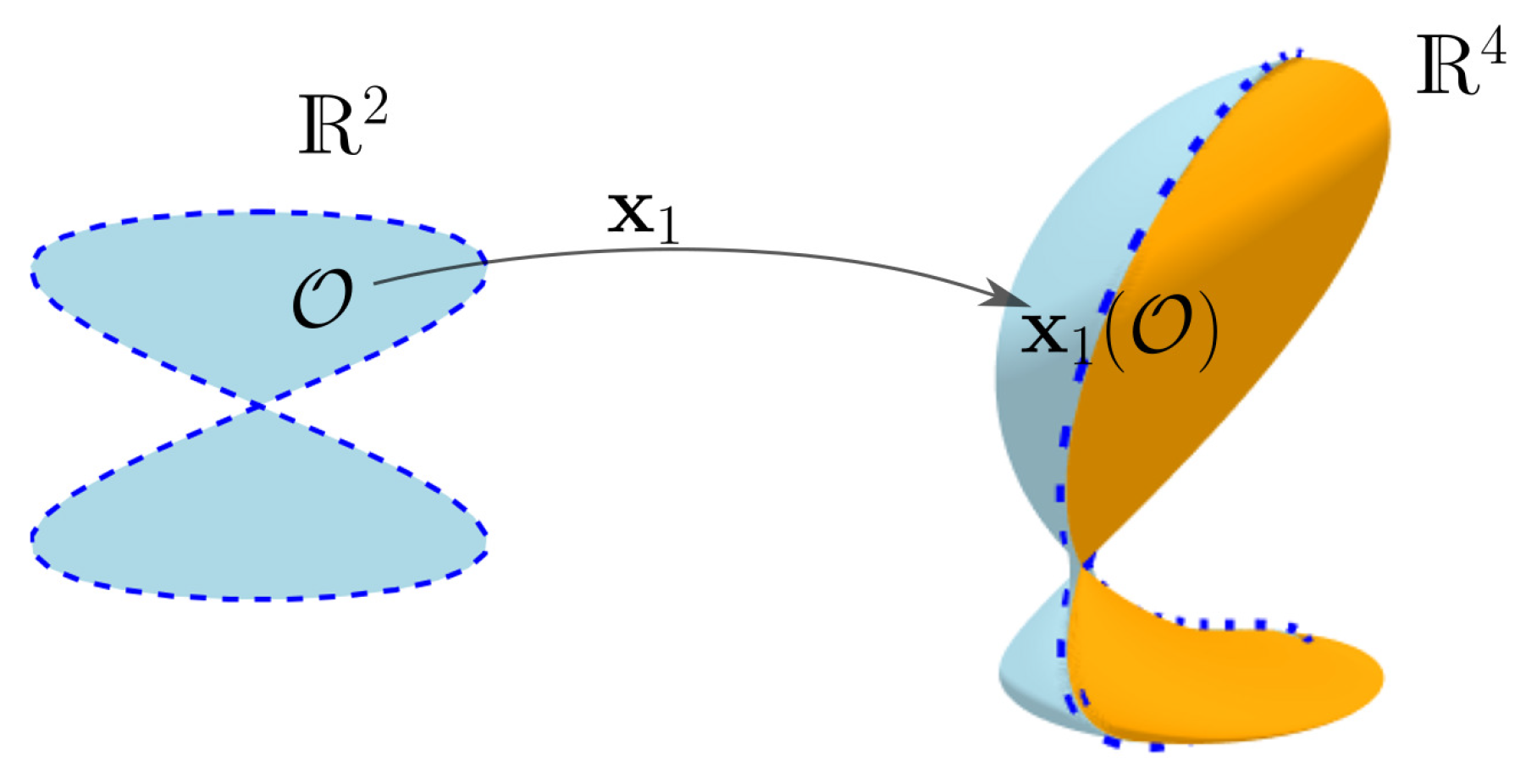
Figure 2.
Sphere centered at with radius , representing the projection of the set M onto the subspace .
Figure 2.
Sphere centered at with radius , representing the projection of the set M onto the subspace .
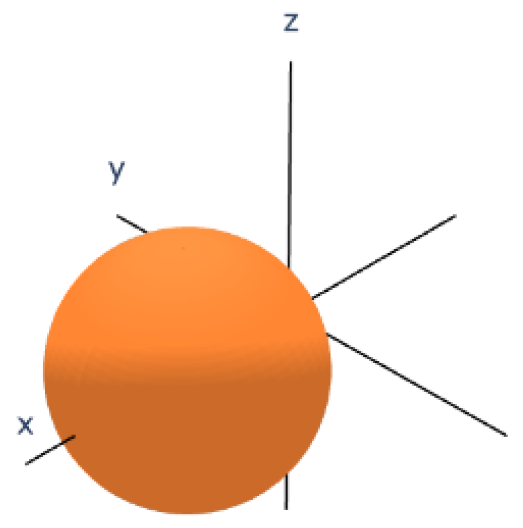
Figure 3.
Cylindrical surface with parabolic directrix .
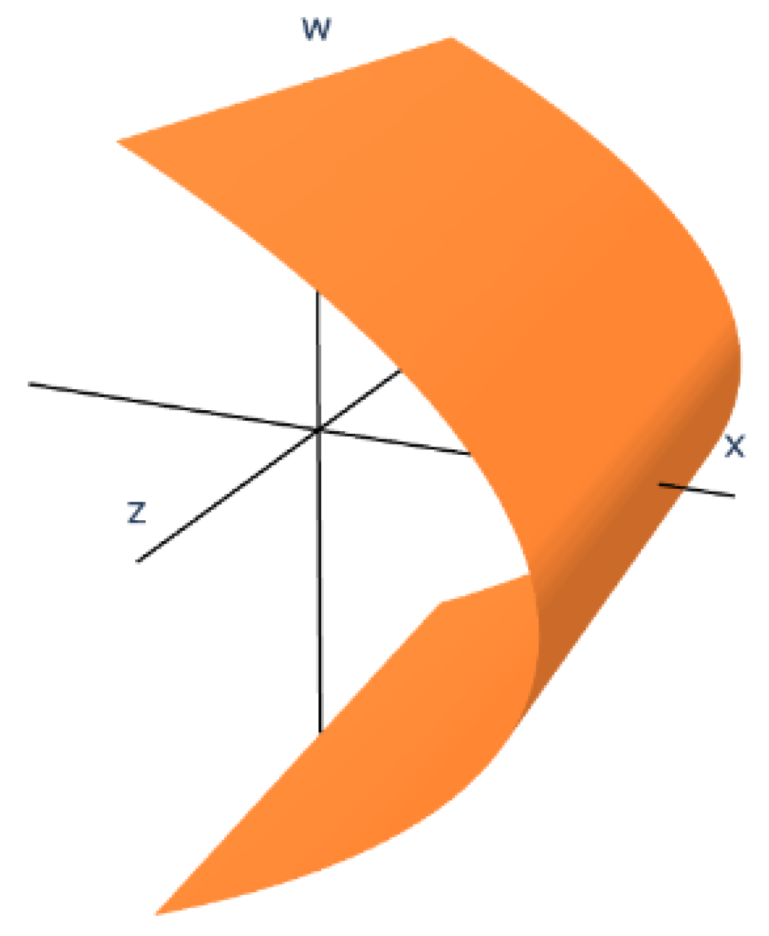
Figure 4.
Algebraic surface of degree 4 defined by .
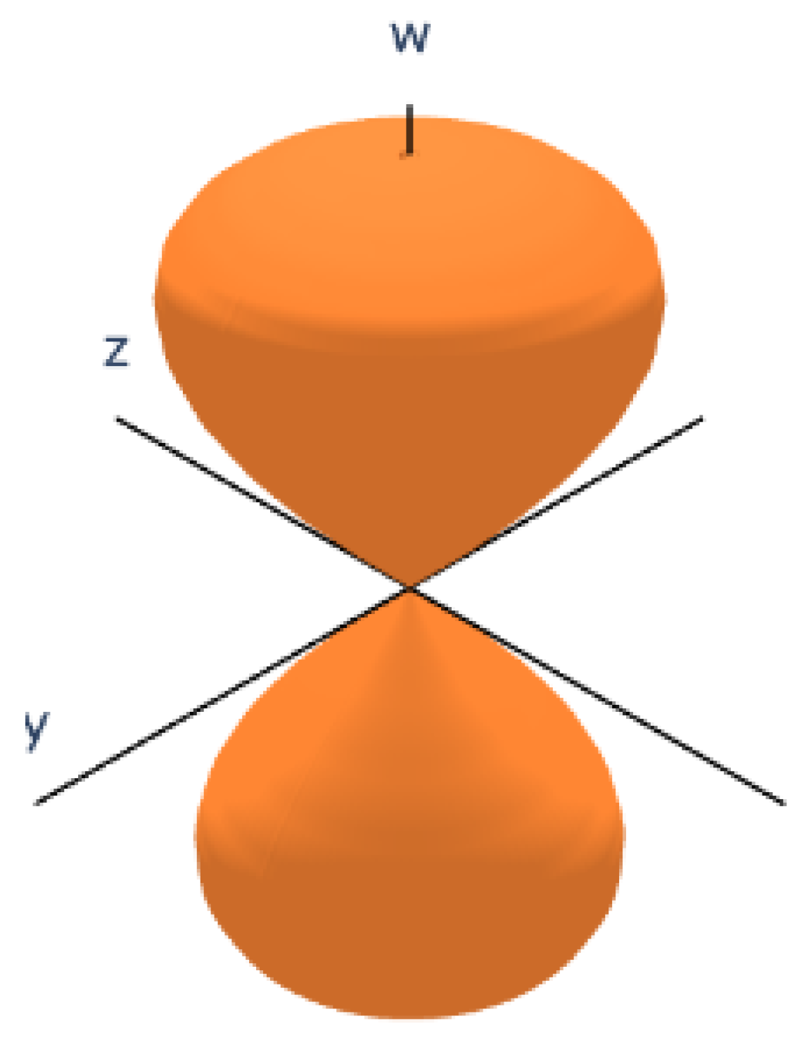
Figure 5.
Three-dimensional projection of the NURBS control mesh defining the Viviani surface in . Colors distinguish mesh directions.
Figure 5.
Three-dimensional projection of the NURBS control mesh defining the Viviani surface in . Colors distinguish mesh directions.
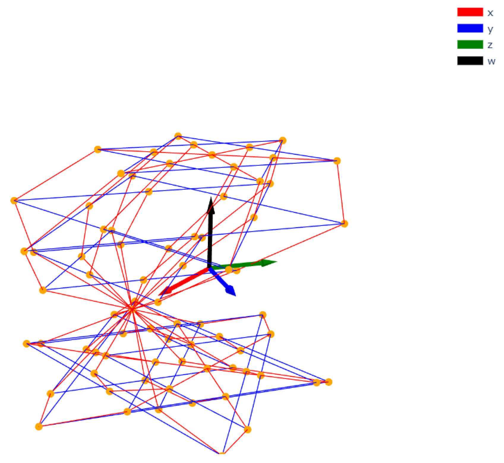
Figure 6.
Plot of the mapping projected to .
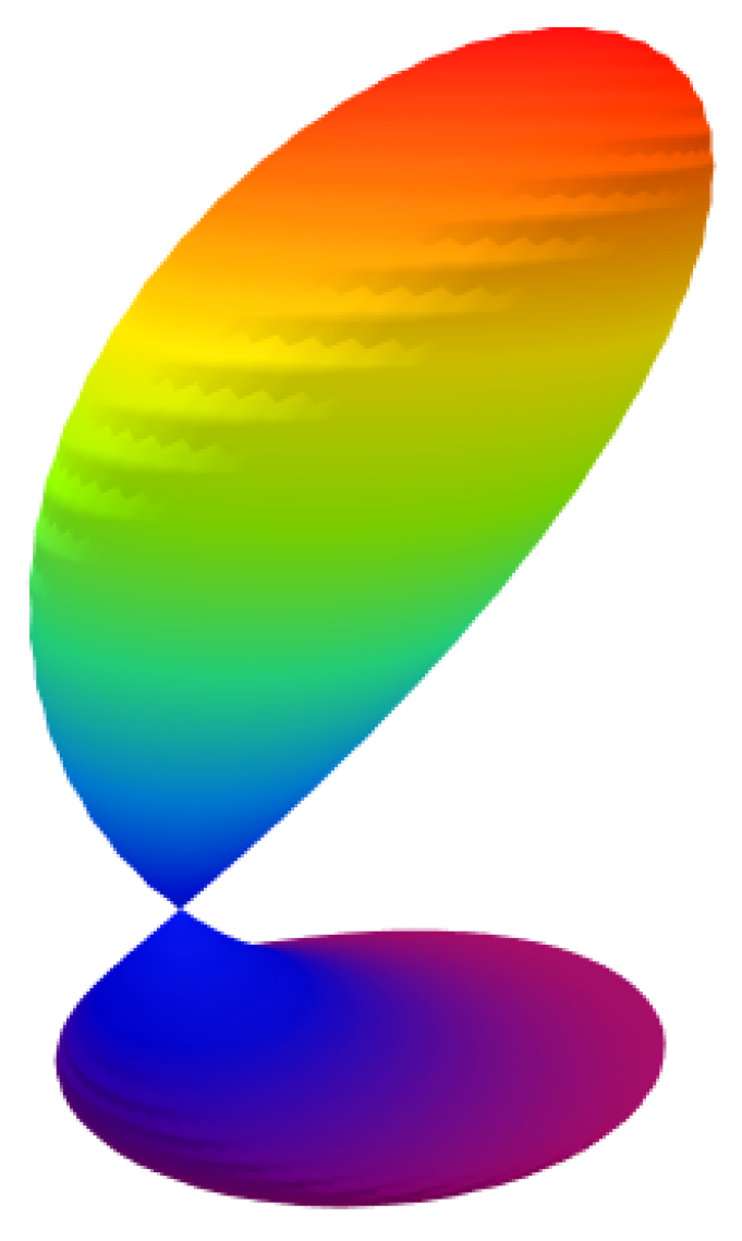
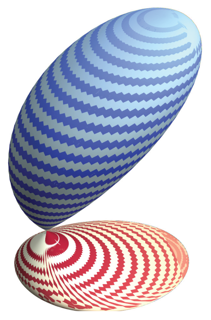
Figure 7.
Smooth polygonal visualization of the NURBS-evaluated Viviani surface projected onto , using a parameter-based color gradient.
Figure 7.
Smooth polygonal visualization of the NURBS-evaluated Viviani surface projected onto , using a parameter-based color gradient.
Disclaimer/Publisher’s Note: The statements, opinions and data contained in all publications are solely those of the individual author(s) and contributor(s) and not of MDPI and/or the editor(s). MDPI and/or the editor(s) disclaim responsibility for any injury to people or property resulting from any ideas, methods, instructions or products referred to in the content. |
© 2025 by the authors. Licensee MDPI, Basel, Switzerland. This article is an open access article distributed under the terms and conditions of the Creative Commons Attribution (CC BY) license (http://creativecommons.org/licenses/by/4.0/).
Copyright: This open access article is published under a Creative Commons CC BY 4.0 license, which permit the free download, distribution, and reuse, provided that the author and preprint are cited in any reuse.


