
Submitted:
27 May 2025
Posted:
27 May 2025
You are already at the latest version
Abstract
This paper presents a new IoT sensory system called SmartBarrel. The system can record wine fermentation attributes and parameters, acting as an electronic nose and tongue. The IoT devices that pertain to this smartBarrel capabilities are the probing nose and tongue devices, which can be easily attached to stainless steel wine barrels. These devices can periodically monitor fermentation parameters, including gas emissions from the nose and acidity, residual sugar, and color changes in the tongue. Nose and tongue IoT devices utilize low-power, low-cost IoT sensors for this purpose and have been validated in small wine fermentation tanks. Apart from the end node devices, the proposed system features a distributed cloud architecture incorporating open-source, industry-ready application services and tools, specifically the Thingsboard platform supported by a NoSQL Cassandra database for data storage and visualization. The authors developed and experimented with a deep learning auto-calibrating variable layer-length, variable cell LSTM recurrent neural network predictor, called V-LSTM, and a fuzzy controller model to analyze wine fermentation processes, provide fuzzy encoded attribute responses, and infer predictions of the fermenting wine alcoholic content concerning other parameters. The results of this approach were compared with existing machine learning techniques in the literature of shallow MLP classifiers, demonstrating an improvement in minimizing RMSE loss of at least 45%. The authors also indicate that their model can be easily adapted into a service capable of issuing breakpoint alerts and adapting to changes to the non-linear characteristic curves of wine fermentations.
Keywords:
Precision Winemaking
; Decision Support Systems
; IoT
; embedded systems
; Agriculture 4.0
; classification algorithms
; Convolution Neural Networks
; Wine fermentation process
; Deep Learning
1. Introduction
The continuous growth of the wine market necessitates the development of higher-quality wine products through standardized industrial processes and the use of IoT. Continuous supervision, control, and implementation of standardized intervention procedures during the alcoholic fermentation of must for wine production are central to the Winemaking Industry. With the advancement of the Internet of Things (IoT) and aligned with Industry 4.0 objectives to optimize winemaking processes, numerous innovative solutions for IoT Systems, data acquisition, and control are being designed and implemented. In this direction, this paper proposes using an AI-capable, low-cost wine fermentation monitoring system to develop a prototype wine fermentation tank that continuously records critical parameters. It will integrate low-cost, energy-efficient embedded sensors for real-time data collection, including key oenological metrics (e.g., fermentation curve measurements, brix levels), turbidity/clarity via color measurements, and monitoring released gases during fermentation.
In wineries, the industrial process of monitoring alcoholic fermentation typically involves manual sampling and laboratory analysis for quality control and decision-making. Generally, this can be performed no more than twice per day. For large-scale wineries, such an approach is practically infeasible for all fermentation tanks, risking stalled fermentations or quality degradation. Continuous close-to-real-time data logging via low-cost in-tank fermentation sensors could significantly improve processes by taking actions on event occurrence, enabling real-time fermentation rate control, enhancing automation levels, and optimizing workforce allocation to higher-priority production tasks. Continuous monitoring via in-tank sensors could streamline fermentation rate control, boost winery automation, and reduce labor overhead, freeing personnel for other production processes. Although embedded sensors (even rudimentary ones) are not novel, their systematic deployment remains restricted, particularly in Greece.
To this extent, the wine industry poses requirements for using dense wine parameters monitoring utilizing device solutions for small-scale wine-fermentation tasks of unsupervised control [1]. There is an urgent need for integrated sensor systems capable of routine measurements and micro-scale fermentations in wineries. The use of basic embedded tank sensors has seen limited adoption, primarily due to cost constraints and the complexity of local monitoring technological integration [2]. There is growing interest from wineries, sensor manufacturers, and startups in incorporating innovative, scale-up, automated enological solutions. Existing industrial fermentation control systems provided by Programmable Logic Controllers (PLCs) of time-interval periodical probing and on-demand supervisory control, as well as via local data acquisition (SCADA) interfaces, have achieved initial production automation [3]. However, Industry 4.0 introduced scalability, portability, and autonomous cloud operation principles of telemetry devices, Ubiquitous IoT connectivity, distributed storage, and intelligence [4], which are still ahead. In order to show progress in this direction, dense, close-to-real-time multi-attribute monitoring is needed using cloud-based services and data collection on preferable schemaless NoSQL databases. This way, the end-user integration provided by notification channels and intelligent, automated suggestions using Artificial Intelligence will offer Industry 4.0 sensory automated processes [5,6].
Wine fermentation processes supported by systems of low-cost deployment using IoT, extensibility, and cross-platform visualization (via tablets/smartphones) are pivotal. Real-time statistical analysis and AI-driven decision support—including oenological intervention recommendations and final product quality predictions—will further advance Wine Industry 4.0 resilience and sustainability. Implementations of periodic and real-time Industrial IoT (IIoT) monitoring systems for measurement supervision, detection-prediction, and decision-making (Decision Support Systems - DSS) is crucial for the primary sector, particularly in biological system supervision [7,8,9,10,11,12]. Nevertheless, despite the importance of such technological tools as applied in other European wine-producing countries (e.g., Spain, Italy, France), Greece lacks comprehensive systems for monitoring wine fermentation, relying instead on static and sporadic measurements using existing instruments developed and tested by European nations.
Towards Industry 4.0 automation, Li et al. propose a new chemical analysis system during wine fermentation consisting of temperature, pressure, pH, and a refractometer [13]. Also, authors at [14] evaluate the use of the MQTT protocol for use in the Wine industry real-time data transmissions. Other propositions include monitoring wine fermentation using biosensors mainly on basic parameters like temperature [15,16], sugar concentration [15,17], acidity [18], bioreactors content, CO2 emisions [19], phenolic compounds [20], and odor characterization [21,22], minimizing microbiological risks [23,24]. State of the art IoT trends include Electronic noses (E-noses) that focus on tank gas monitoring [19,25,26,27,28,29,30], Electronic eyes (E-eyes) that utilize RGB and IR monitoring) [1,30,31,32,33,34] and Electronic tonques (E-tongues) for in tank basic paramters monitoring [15,19,29,30].
Mathematical and statistical methods are the necessary tools to mine and extract valuable information from large datasets. These methods, in turn, enable predictive modeling and continuous improvement, thus enhancing production flexibility. Process optimization requirements cannot be standardized for dynamic systems. Such procedural behavior can be monitored and measured with modern techniques and facilitated with precise operations. Machine and Deep learning applications in natural sciences facilitate the development of intelligent decision-support systems. Daily time-series data from processing units serve as input for machine support models. Mathematical algorithms including Neural Networks (ANN), SVM, Random Forest, Logistic Regression, XGBoost, CNN classification models such as UNets, ResNets and VGGNets, Multilayer Neural Networks (e.g., Stranded-NN [12,35]) and predictive Recurrent Neural Networks (Stranded-LSTM [36]), as well as Fuzzy Logic models[12,37,38] operating as autoencoders in cases of limited data availability. Such models have been investigated for prediction and classification tasks for wine fermentation tasks, offering predictions and criticality alerts [7].
From this perspective, the authors propose a new low-cost architecture supported by probing electronic nose, tongue, and eye devices, which are incorporated into autonomous devices using a holistic system approach called SmartBarrel. These devices offer an electronic sense of the corresponding sense (nose, tongue, eye) and are named probing nose, tongue, and eye (probing, E-nose, E-tongue, E-eye). The SmartBarrel prototype utilizes low-power wireless IoT application protocols for data transmission, following HTTP JSON POSTS over Wi-Fi [39], implements streamlined close to real-time cloud-based transmission of measurements via the portable, easy-to-install probing devices, reducing the application costs utilizing existing tank-stationary sensory solutions. Additionally, it integrates deep learning for measurement validation, predictive analytics, and intervention alerting mechanisms.
In short, the SmartBarrel prototype system incorporates 1) Measurements acquisition via the ThingsBoard AS [40], 2) deployment of intelligent fermentation process and models, 3) automated prediction of subsequent fermentation phase, 3) alerts and notifications for undesirable fermentation cases, and 4) ubiquitous monitoring via its cloud-based AS ability to illustrate real-time measurements, alerts and predictions with the use of a mobile phone application, enabling ubiquitous monitoring of oenological processes.
These cloud-driven SmartBarrel capabilities offer the building blocks for the next generation of innovative winemaking tools. In this respect, the present work includes the following sections. Section 2 presents a systematic review of the available literature on emerging technologies used for wine fermentation conditions monitoring and detecting critical events. Section 3 presents the authors’ proposed SmartBarrel high-level system implementation, prototype end IoT devices implementation, deep-learning cloud computing predictions of the fermentation process based on a new RNN model called V-LSTM, and ThingsBoard application-level protocols and interfaces. Section 4 presents the experimental scenarios of the system’s and V-LSTM model evaluation, and Section 5 concludes the paper.
2. Related Work
Several implementations have been presented in the literature over the last few years regarding small-scale fermentations in tanks assisted by monitoring systems and IoT devices. Most of them target capturing the sense of smell, touch, and vision more precisely than the human senses. Analyzing gases released during alcoholic fermentation uses Fourier Transform Infrared (FTIR) systems or scattering spectrophotometers. These high-cost instruments (exceeding $20,000 per unit) require manual operation and complex maintenance, limiting their use to periodic sampling rather than continuous or close-to-realtime monitoring. At the research level, electronic nose (E-nose) systems have been investigated for gas/volatile compound detection [41].
Most E-nose implementations rely on conventional sensor configurations, including conductive polymer sensors (CPS), metal oxide semiconductor (MOS) sensors, as well as acoustic and optical sensors [25]. Four principal sensor types prevail: 1) The MOS sensors that detect resistance variations from electron transfer during gas adsorption [28], 2) the catalytic ga sensors (CAT) measure capacitance changes [42], 3) the electrochemical sensors (ECH) that utilize charge transfer measurements in electrolytic cells [30] and 4) other types such as infrared sensors [43].
Electronic nose systems have shown particular promise for volatile aroma compound analysis, demonstrating the capability to differentiate wines based on aromatic profiles [27,44,45], or detecting Volatile Organic Compounds (VOCs) [46]. Furthermore, research-grade E-nose systems have been deployed directly in fermentation tanks, enabling online parameter monitoring [47]. Most implementations include low-cost MOS sensor arrays for alcohol, CO2, H2S, and SO2 detection [26,27,28,48]. These MOS-type sensors have been successfully employed for monitoring alcohol and CO2 gas concentrations during fermentation of Debina, Zitsa, Greece, and white grape variety [30].
Nevertheless, Electronic nose sensors face several challenges, including reduced chemical selectivity, limited sensitivity, and susceptibility to temperature and relative humidity (RH) variations. However, their low cost and reasonable effectiveness in array configurations [28] make them attractive for integration in the SmartBarrel system’s E-nose module, particularly when combined with machine and deep learning models for aroma characterization [27,44,45].
Electronic tongue systems constitute artificial analytical instruments designed to replicate human gustatory perception. These devices typically incorporate sensor arrays for acidity, sugar content, alcohol levels, and organic compounds such as polyphenols, which, when combined with chemometric processing, enable comprehensive characterization of complex liquid samples [29,46,47]. The classification and determination, including quantitative analysis, of grape varieties from must and wine blends represent significant interest for winemakers, as it facilitates precise quality control and product differentiation throughout the production process.
The alcoholic fermentation process and its characteristic curve, including essential measurement parameters such as sugar content (Brix-specific gravity), temperature, pH levels, and alcohol concentration, are considered critical determinants of vinifiable product quality, necessitating continuous monitoring throughout winemaking [29]. Additionally, spontaneous releases during fermentation are important monitoring process parameters that address this requirement [49].
Finally, Electronic eye systems capabilities integrate voltammetric electrodes [50,51], enabling rapid organoleptic assessment of wine samples outside the fermentation tank. Visible-near infrared (Vis-NIR) spectroscopy has been employed for polyphenol analysis in winemaking [34,52]. However, current implementations rely on offline sampling methodologies rather than the continuous in-tank monitoring proposed by this system. Integrating these complementary analytical approaches within a unified monitoring platform significantly advances conventional discontinuous quality control practices in the wine industry [32]. Furthermore, an air CO2 bubble gas capture sensor implementation that utilizes images and Deep learning CNN detection is presented in [53].
The evaluation and regulation of winemaking parameters towards wine quality, using E-eye technologies, will achieve significant results through tannin quantification (detection at 1600nm wavelength) influencing the phenolic profile, along with must aromatic compound analysis (spectral detection at 1100-1300nm range) [31]. Monitoring polyphenol evolution during different wine production stages proves critical for premium quality wine output. To this extent, E-eye sensory subsystems operating in selected visible (VIS 460-680nm) and near-infrared spectral bands (NIR band-a 1100-1300nm, NIR band-b 1580-1620nm) can enable real-time Total Polyphenol Index (TPI) estimation [25,33]. These optical monitoring capabilities provide unprecedented potential for continuous phenolic maturity assessment during vinification, allowing winemakers to make data-driven interventions at optimal tannin extraction and aromatic preservation time points. The combined spectral analysis of visible color characteristics and near-infrared molecular signatures represents a technological advancement over current discontinuous laboratory sampling methods, particularly for phenolic compound management in red wine production, where extraction kinetics significantly influence final product quality. The following Section 3 presents the authors’ SmartBarrel system implementation incorporating Electronic nose and tongue capabilities, as well as limited Electronic eye capabilities.
3. Materials and Methods
The authors present a new fermentation monitoring system called SmartBarrel. They present the high-level system architecture, followed by the sensory parts and capabilities of the end devices. The proposed system has been evaluated for its data delivery processes. The authors also propose a fuzzy control monitoring process for fermentation alcohol predictions and a fuzzy autoencoder for fermentation data acquisition needed by their proposed deep learning V-LSTM model, which offers future fermentation measurement predictions based on previously SmartBarrel-measured parameters.
3.1. SmartBarrel System Architecture
The proposed SmartBarrel system has been designed to provide the necessary flexibility for sensor integration, enabling holistic, intelligent control of vinification processes with low-cost electronic sensor monitoring. Beyond basic parameters measurement during alcoholic fermentation, the SmartBarrel system includes intelligent processes and real-time measuring and monitoring capabilities accessible from any location within the winery facility. It implements analytics and interactive monitoring functionality via appropriate device-level user interfaces. The high-level system architecture of SmartBarrel is illustrated in Figure 1.
Figure 1.(1) illustrates the fermentation case implementation where the SmartBarrel IoT end node probes reside (E-nose, E-tongue) collecting fermentation measurements. Those measurements are collected to an appropriate MPU controller (see Figure 1.(2)). The MPU controller connects over Wi-Fi to the cloud ThingsBoard Application Server (AS, Figure 1.(3)), sending telemetry data periodically using either HTTP or MQTT posts. Then, the ThingsBoard AS and the ThingsBoard mobile phone application are responsible for visualizing fermentation measurements per device tank-id using appropriate dashboards (Figure 1.(4)). The collected data can be accessed using server-side RPC MQTT requests to collect specific time interval, device and attribute measurements. This selectivity of measurements is used as input to provide inferences by the deep learning V-LSTM model predictions, posted back to the ThingsBoard as JSON predictive data measurements, and illustrated via appropriate device-assigned dashboards. Figure 1.(5) illustrates the ThingsBoard mobile device where they can access and visualize the measurement data remotely. This high-level architecture is a simplified approach to the thingsAI platform presented in [11,12].
SmartBarrel end node equipment includes an E-nose and E-tongue IoT device on the floating lid of small stainless steel fermentation tanks. The current SmartBarrel system implementation is only the E-tongue sensor subsystem for real-time measurement of fundamental oenological parameters of pH, sugar concentration, and temperature, and an E-nose sensors ring that is comprised of monitoring gas emissions of ethanol, CO, and CO2. An RGB color sensor with incorporated LED has been added to the E-tongue device to introduce the E-eye capability to this preliminary system. This color sensor is used to monitor wine clearness and color transitions. Finally, a glass brix meter device is used for sugar concentration measurements floating inside the wine tank, with an analog capacitive touch sensor attached. Since new NIR sensors and transducers must be added to have a proper E-eye device, its final implementation, validation, and experimentation are set as future work.
Concluding, the proposed system includes the following components, sensors, and actuators:
- E-tonque end node IoT device: This is the end node device that includes a pH meter, a brix meter, a pressure, and a temperature sensor
- E-nose end node IoT device: This includes the MQ-3 (Alchohol) and MQ-7(CO) sensor, MG811 carbon dioxide sensors, as well as temperature sensors
The proposed SmartBarrel system’s integration of such multisensory data with fermentation parameters provides unprecedented capabilities for real-time oenological decision-making. During fermentation, measurements are collected in a cloud-based open-source ThingsBoard Data Acquisition System [40], enabling real-time visualization and statistical processing/analysis. Specifically, the system incorporates four key interfacing capabilities: 1) Visualization and statistical processing of collected measurements, 2) correlation functions implementation using selectable parameters and visualization of the results over time intervals, 3) execution of external inference processes provided by Deep Learning models on selected collected measurements and display of classification/prediction results, 4) based on the predicted results, threshold-based algorithms that connect to predefined text alerts and notifications of recommended oenological interventions. With the ThingsBoard mobile phone application, these visualizations can be available, even outside the industrial winery environment.
The ability of the SmartBarrel to collect data to the cloud makes it easy to implement, cloud-based machine, and mostly deep learning algorithms capable of periodic classification/calibration of wine quality parameters (visual, olfactory, and taste characteristics). Predictive assessment of fermentation stages through deep learning, generating alerts for undesirable fermentation deviations and providing interactive intervention suggestions on outlier values. Finally, automated parameter correction is performed when values exceed predefined thresholds, ensuring optimal fermentation conditions throughout the process. The SmartBarrel system integrates these functionalities through a unified IoT architecture, combining cloud computing for real-time response with cloud-based analytics for long-term process optimization and quality enhancement. An analytical description of the SmartBarrel end-node devices follows.
3.2. SmartBarrel End-Node Devices
The SmartBarrel end node device consisted of two different probing equipment as designed. A probing nose inherits the Electronic nose functionality, and a probing tongue inherits the Electronic tongue functionality. Partially, Electronic eye functionality has been implemented into the Electronic tongue. Therefore, the two IoT end-node devices (nose, tongue) acquire the following sensing capabilities:
- E-nose: Monitoring of CO gas emissions inside the fermentation tank
- E-nose: Monitoring of CO2 gas emissions inside the fermentation tank
- E-nose: Monitoring of alcohol gas concentrations inside the fermentation tank
- E-nose: Monitoring lid air temperature inside the fermentation tank
- E-nose: Monitoring yeast temperature using a stainless steel temperature probe
- E-tonque: Monitoring temperature and pressure values in the air gap inside the tank
- E-tonque: Monitoring fermenting wine specific gravity by performing electronic hydrometer measurements that indirectly correspond to sugar concentrations through density. That is, for liquids heavier than water, Equations 1 apply:
- E-tonque: PH meter and temperature sensor for yeast PH and temperature-pressure measurements
- E-tonque: RGB sensor with LED for capturing the color of red wines that anthocyanins are responsible for the red and purple color of wines, while tannins contribute to color stabilization and astringency perception [54] (white wines have low tannin concentrations and absence of anthocyanins [55]). On the other hand, to capture the oxidation of phenolic compounds, leading to yellow, gold, or brown hues over time, and cinnamic acids and other hydroxycinnamates (e.g., caftaric acid), which can undergo enzymatic oxidation and contribute to wine browning [56,57,58].
3.3. SmartBarrel E-Nose Device
The SmartBarrel E-nose device is illustrated in Figure 2, attached to the stainless steel lid of the fermentation tank of typical sizes from 50-500lt.
Figure 2.(11) shows the E-nose placement to a 75lt 36” lid. Figure 2.(1) is the plastic case screwed to the lid’s ventilation hole via a plastic rod. (Figure 2.(2)). Figure 2.(3) is the DS18B20 temperature sensor measuring lid temperature, end Figure 2.(5) is the devices DS18B20 temperature sensor probe that is inserted inside the fermenting wine measuring liquid temperature. Figure 2.(4) is the MG811 CO2 sensor typically measuring ppm in the range of 300-10,000. It is an electrochemical sensing analog device, and it is attached to the microprocessing unit’s (MPU) 10Bit analog-to-digital converter (see Figure 2.(8)). Similarly, Figure 2.(7),(6) are the MQ-3 alcohol and MQ-7 CO sensors accordingly. These two analog MOS sensors measure resistance changes due to chemical reactions between gas molecules and the MOS surface. Typically, MQ-3 measures up to 0-20mg/L alcohol in the air while MQ-7 up to 2000ppm of CO in the air and is connected to the MPU unit via its analog-to-digital (A2D) converter.
The sensors are connected to an Arduino Wi-Fi rev.2 MPU, a Microchip ATmega4809 8-bit microcontroller with a 16MHz clock, 48KB of program memory, and 6KB of SRAM. It also includes a u-blox NINA-W102 Wi-Fi transponder and an LSM6DS3TR Inertial Measurement Unit (IMU) (see Figure 3.10). The device is powered using a DC-12V transformer and transmits periodically every 5-minutes measurements of temperature (internal and lid-external), CO, CO2, gas alcohol concentrations inside the fermenting tank, using either HTTP/POSTs or MQTT, of JSON encoded telemetry data. Another MPU device of the same microcontroller is used by the SmartBarrel E-tongue device to transmit telemetry data, as described in the following section.
3.4. SmartBarrel E-Tongue Device
The SmartBarrel E-nose device is illustrated in Figure 3, attached to the stainless steel lid of the fermentation tank. Figure 3.10 illustrates the plastic enclosure of the Arduino Uno Wi-Fi MPU, attached to the tank’s ventilation hole
On the inner surface of the lid, the pH probe (Figure 3.(6)) has been attached (screwed) to the ventilation’s hole plastic winding via a flexible sink hose (see Figure 3.(3)), with a plastic curved tube inserted in the hose opening (see Figure 3.(4)) for the fermentation CO2 to escape the tank via its ventilation hole. The pH sensor is an analog sensor capable of measuring from 0 to 14. It is connected to the MPU’s 10-bit analog-to-digital converter via a BNC connector board with an op-amp amplifier and a voltage regulator. Figure 3.(7) is the analog Baume sensor that includes a capacitive liquid level sensor meter attached to a sealed glass tube hydrometer capable of measuring Baume degrees that correspond to Brix units and, therefore to sugar concentrations on g/L (see Equations 1).
An I2C MS5803 pressure-temperature sensor is attached to the curved tube (see Figure 3.(4)) capable of providing temperature and pressure measurements inside the tank for the tongue probe. Finally, the adafruit I2C TCS34725 RGB sensor (see Figure 3.(2)) enclosed in a plastic transparent case is used to get RGB color measurements from the fermenting wine. In order to obtain color measurements inside the tank, the sensor’s attached RGB LED opens and stays on for 30 seconds before acquiring a color measurement. The analog and I2C digital sensors are connected to the Arduino Wi-Fi rev2 board that, in turn, transmits them every 5 minutes to the ThingsBoard AS using either HTTP POST or MQTT publish messages of JSON encoded measurements. Before presenting the authors’ experimental scenarios and their proposed fuzzy inference, data encoder, and V-LSTM model, the metrics used to evaluate them are outlined in Section 3.5.
3.5. Evaluation Metrics
Prior to presenting the SmartBarrel fuzzy controlled fermentation inference process and GRU deep learning prediction process, the evaluation metrics used are the following:
- Root Mean Square Error (RMSE). It is calculated based on the formula 2.where denotes the actual value, is the predicted value, and n is the total number of observations. RMSE calculates the average magnitude of the prediction errors and penalizes large deviations more than smaller ones due to the squaring operation. The minimum value of RMSE is 0, which indicates perfect prediction. Higher RMSE values indicate larger deviations between predictions and actual values. Outliers in RMSE typically arise from large individual prediction errors and disproportionately affect the score due to squaring. Thus, RMSE is highly sensitive to extreme values.
- Coefficient of Determination () shows how well the model explains the variance in the predicted variable based on the inputs. It measures the proportion of the total variation in the data captured by the inference results. It is calculated according to Equation 3where, is the actual value, is the predicted value, expresses the mean of the actual values, and n is the number of samples. The maximum value is 1, indicating perfect prediction. If close to 0, it suggests poor model inferences. Negative values can also occur when the model performs worse than a simple mean-based prediction. Extreme negative values usually signal serious model misfits.
3.6. Proposed Fuzzy Alcohol Controller
The authors implemented a fuzzy controller logic that can even be implemented at the device level (edge computing) [59] to provide a fuzzy inference mechanism of alcohol concentration in the tank. The controller inputs our E-tongue and E-nose measurements and infers alcohol concentration measurements. In order to achieve this, appropriate fermentation datasets (25 white wine fermentation curves) have been used to train the fuzzy controller. Upon training and hyperparameter calibration, the fuzzy controller can provide alcohol predictions on measurements similar to those trained. This inference process is then passed to a Gaussian filter for smooth time-series responses. By using the fuzzy controller, the alcohol concentration values can be inferred.
Looking at the fuzzy controller implementation, the Gaussian membership function is used in the fuzzy sets, ranging between 0 and 1. The parameter mean is the center of the Gaussian curve, where the membership is maximal and equal to 1. The parameter is the standard deviation, which controls the width of the bell-shaped curve. A smaller results in a narrower curve, while a larger produces a wider, flatter curve. To take into account distribution skewness (to the left or the right), the median value is taken into account. The difference between mean and median is the right or left skew factor of the Gaussian curve, while the is used to: 1) provide a normalized offset distance value of the gaussian median (expressed as: ) which in turn is used to offset the gaussian curve centers, and 2) as a representative width of the gaussian bell curve used for each random variable.
In order to implement a fuzzy controller that takes as input wine fermentation parameters acquired by the SmartBarrel implementation and infer a real-time alcohol value, an appropriate fuzzy controller has been implemented using as inputs measurements of the following wine attributes:
- Sugar concentration in (g/L)
- pH measurements
-
CO2 concentration expressed in g/L. Let be the concentration of carbon dioxide produced during fermentation intervals dt, and let be the equivalent concentration of it expressed in parts per million. The conversion is expressed by Equation 4:Since ppm is used to express air concentrations, let be the concentration of CO2 floating inside the tank at a specific time interval dt, we use Henry’s law which describes the solubility of a gas in a liquid by Equationwhere is the concentration of dissolved CO2 in fermenting wine (mol/L), is Henry’s law constant for CO2 in white wine, approximately at 20°C (lower than water which is ), and is the partial pressure of CO2 in atm. Substituting , and converting from mol/L to g/L, by multiplying with the molar mass of CO2 (44.01 g/mol) the final Equation 6:provides the concentration of CO2 inside the fermenting wine. Concluding the ratio of CO2 concentrations in the liquid over the air under equilibrium conditions is expressed by Equation 7This equation allows estimation of the CO2 content in fermenting white wines from ppm gas-phase concentrations under standard conditions. That is, the mass concentration of CO2 in fermenting white wine over time is approximately 37% of the mass concentration in the gas phase.
- Biomass fermentation residues. It includes any form of a specific product or metabolite and substances already included in the must that take part in the fermentation process. The development of particular components or biological decontamination can be measured by weighting the solid state extracted material from the fermenting wine (in g/L) during the controlled decantation of wine from one vessel to another, which is primarily aimed at separating it from lees and sediment, thereby enhancing its clarity, microbiological stability, and overall sensory purity.
- Temperature of the fermentation process (maintained constant) in .
- Alchohol concentration measured in g/L. The alcohol concentration is the output variable (consequent), while all others are input variables (antecedents).
These measurements have been obtained using the dataset provided from [60], which included fermentations of white grape yeast. Given a dataset with column X representing an antecedent, We assume that all input variables follow a Gaussian or a Gaussian skewed distribution during fermentation, except temperature, which follows more of a constantly controlled profile. We define the following statistical measures:
where is the arithmetic mean of X.
representing the median value of X.
denoting the sample standard deviation (ddof=1) of X. The median and mean are the measures used to provide the mean, which is sensitive to extreme values, and the median is robust to outliers. The relationship between these two measures provides insight into the skewness of a distribution. We also define a dispersion parameter according to the following Equation 11:
Using Equation 11, the normalized skewness adjustment parameter is computed for each variable according to Equation 12:
Given the dataset D, of N timeseries attributes denoted as: , where each is a time series attribute of length T, given by:
Then, , input data measure denoted as attribute three Gaussian membership functions are constructed, for with parameters (centers) expressed by Equation 13:
where contains the centers for each attribute. Each Gaussian membership function for is defined using Equation 14:
where is the minimum observed value, is the mean value from 8, and is the maximum value adjusted by 12. The complete fuzzy partition for an attribute variable x is then given by Equation 15:
where each member of follows 14 with parameters from (13) and bandwidth from 11. Uniform hyperparameters are used across all input attributes MF functions (high, medium, low) to set the appropriate Gaussian curve over the range of accepted attribute values. These parameters are presented in Table 1.
In order to smooth consequtive timeseries of infered alchool value of the fuzzy controller, the Gaussian smoothing of discrete measurements with a boundary mode set to nearest, cant be used and it is computed via discrete convolution where the Gaussian kernel G has standard deviation and the boundary condition enforces for and for , with the kernel weights for truncated at and normalized to sum to unity, such that each smoothed point , replicates the nearest boundary value (nearest neighbor) when the kernel window exceeds the measurements domain.
The following Section 3.6 presents the authors’ fuzzy autoencoder of a time series of fermentation parameters to create a first-stage Recurrent Neural Network capable of generalization of prediction of fermentation curves from historical data. Experimentation with the fuzzy inference controller implementation is presented in Section 4.2.
Fuzzy Fermentation Autoencoder
In order to provide fermentation parameters predictions, a time series of a dense number of parameter measurements is required. These datasets should have minute scale resolutions for the deep learning RNN models to minimize losses and offer accurate results. Only machine learning approaches, such as decision tree-based predictors (LightGBM) or SVR machines, are available if such data are available in more than hourly periods. Focusing on white wine fermentation processes, and since such dense datasets are not yet widely available to train RNNs, the authors focus on an autogenerated approach provided by a fuzzy autoencoder that combines fermentation parameters knowledge from literature [13,49,50,61,62], accomodated small sets of collected dataset of wine fermentations, such as the acquired data from the SmartBarrel system, to fuzzy generate fermentation data sequences. The fermentation encoder is modeled through fermentation phase-dependent fuzzy rules [63], implementing the following attributes:
- Temperature is strictly controlled regardless of phase following white wine fermentation temperatures
- Alcohol production correlates with biomass and sugar, but it is calculated using the fuzzy controller as a predictor, as mentioned in Section 3.6
More specifically, the authors use the mathematical formulation provided by Equation 16 to describe parameter dynamics during the fermentation phases.
where the membership functions for each one of the fermentation phases are defined according to Equation 17:
The trimf is the triangular membership function and its corresponding parameters (start, peak, end), trapm the trapezoidal membership function and its corresponding parameters (start of rise, top start, end top and fall end), and smf the S-shaped membership function and its smoothly increased parameters from 0 to 1, a,b accordingly.
The biomass concentration is used since it is mentioned in [60], of the provided white wine fermentation curves and monitored by the SmartBarrel system by weighting the removed solid residues of the wine in each wine clarification steps (4-6 during the fermentation process). This parameter kinetics in g/L is modeled using a phase-specific growth kinetics Equation 18:
where g/L is the Initial biomass, h is a Lag time constant, g/L is the maximum biomass as recorded, h−1 is the growth rate, h is the exponential fermentation midpoint, g/L/h is the decline rate, h−1 is the death rate and is the noise process term. The sugar concentration exhibits complementary phase behavior with respect to and it is modeled using Equation 19:
where g/L is the initial sugar concentration modeled using a uniform distribution (). h−1, is the sugar consumption rate in g/hour (using a uniform distribution ). g/L is the residual sugar, g/L is the transition amount coefficient at the stationary fermentation phase, h−1, is the stabilization stationary phase rate, g/L is the final concentration and is the noise term. Moreover, the fermentation process evolves using the rate equations described in Equation 20:
where is the fuzzy-controlled growth rate and g/g is the yield coefficient. The complete system has been validated against industrial fermentation data. The pH rules have be mathematical formulated according to Equation 21, as mentioned and mechanistically explained in [62]:
Finally, the fuzzy rules based on literature wine fermentation responses that govern the fuzzy autoencoder are presented in Table 2 and further analytically elaborated over fermentation phases and previously expressed equations on Table 3. The noise terms presented in Table 3 are expressed by the Equation 22 bellow:
The described fuzzy controller can provide analytical white wine fermentation parameter curves as modeled using per-phase Equations presented in Table 3. This can lead to dense fermentation datasets generation, except alcohol concentrations that can be inferred using the alcohol fuzzy controller described in Section 3.6 using white wine experimental fermentation curves. This autoencoding process can simulate white wine fermentation processes with minute resolution granularity acquisition of fermentation parameters.
The fuzzy autoencoded datasets, in turn, are used by the authors’ proposed variable cells and layers LSTM model called V-LSTM, presented in Section 3.7. This deep learning model can, in turn, offer future responses to fermentation processes. More precisely, the authors propose an algorithm for fermentation parameter predictions that has historical parameter data as input. Due to insufficient data sources, the fuzzy controller is primarily used as an autoencoder and predictor of alcohol degrees. Until sufficient data collection, the fuzzy autoencoder provides training sets for the V-LSTM model to offer temporary predictions (future fermentation parameter responses).
3.7. Proposed V-LSTM Model
The authors propose a new model for predicting wine fermentation parameters from up to now monitored values of pH, temperature, CO2 tank concentration, sugar, alcohol, and biomass concentrations [60]. The proposed model is an LSTM model with fuzzy autoencoding and self-healing capabilities. Figure 4 illustrates the process steps of the V-LSTM model. Figure 5 illustrates the V-LSTM model structure of variable cells and layers and its corresponding data inputs and outputs.
The V-LSTM model can be trained using two different training modes: a) autoencoding data training mode and b) actual data training mode. The operation mode selection is dependent on use and can be arbitrarily set. As shown in Figure 4, if in autoencoding mode, steps 1,2 and 3 are used to provide actual training data for the model. The actual data training mode assumes that a dataset of timely-dense fermentation measurements has been acquired and moves straight to the Figure 4.4 step of the model hyperparameters calibration.
Figure 4 describes the V-LSTM model framework integrating fuzzy logic and LSTM (Long Short-Term Memory) neural networks for fermentation process modeling and particularly focusing on providing data input parameters prediction in the future, called attributes looking at variable timestep windows of paste measurements. The process begins with collecting a minimal dataset of fermentation parameters such as concentrations of sugar, CO2 biomass, and pH and a set of fuzzy rules that express their inter-relationship in a fuzzy manner. The dataset is used to formulate: 1) An alcohol fuzzy controller, as described in Section 3.6, and 2) a fermentation data autoencoder, as described in Section 3.6. The autoencoder is used to generate dense measurements of fermentation data. At the same time, the fuzzy controller is trained using the minimal dataset and then used to provide alcohol measurement inferences for the data generated by the fuzzy autoencoder.
V-LSTM model training includes also a pre-processing step (see Figure 4.4), that involves the determination of The included LSTM model number of cells is , and the number of layers is l. These hyperparameters are first investigated by performing random searches using, as search parameters, the maximum number of trials and the minimum distance between values over a pre-determined range of cell values (8..512) and layer values (1..10). These values can be manually set at the V-LSTM model. The hyperparameters tuning process ends with selecting the minimum loss cells first and then using that minimum number of cells to select the minimum loss number of layers. The loss parameter investigated is the validation RMSE loss of a portion of the entire dataset used for training and, therefore, validation of the respective LSTM generated models [36]. Upon selection of cells and layers hyperparameters, the final LSTM model is built as illustrated in Figure 5.
The built model is trained over the dataset of k attributes using a pre-selected timestep of historical data window and predictions time length of predictions to infer for that timestep. Then, the dataset time series is loaded to memory and transformed into normalized data using min-max normalization per attribute. The same applies to the dataset labels that include the next timestep min-max normalized data equal in size to the predictions timelength .
Figure 5 illustrates the layer-wise architectural diagram of the V-LSTM (Variable-Length LSTM) model used for time-series predictions. It outlines how input sequences are transformed through stacked LSTMs and dense (NN) layers, reshaped, normalized, and finally mapped to a prediction output.
This V-LSTM model architecture is a hybrid RNN-NN variable size and depth time-series model that takes multivariate sequential 2D array inputs of data, where is the historical time series window of the multivariate data of k attributes. It utilizes pre-tuned l stacked layers of pre-tuned LSTM cells each. Then, it uses two dense NN to smoothly transform the stacked LSTM output of values to and finally to 1D array of consecutive values from the second NN layer. These values are then reshaped to form a 2D () array. This array is the model’s final prediction output. That is, after passing through a batch normalization step to smooth outliers jitter on the prediction value attributes.
In conclusion, the proposed V-LSTM model combines automatic fuzzy data encoding and parameter autotuning processes. It is well-suited for tasks like fermentation process forecasting, sensor data prediction, or any sequential regression application involving fuzzy or biological systems. Section 4.3 also evaluates the authors’ proposed V-LSTM model.
4. Experimental Scenarios and Results
The following subsections present the authors’ experimentation and proposed model evaluation. Scenario I presents the authors’ experimentation with their implemented SmartBarrel IoT E-nose and E-torque devices. Scenario II presents the authors’ experimentation of their SmartBarrel measured fermentation data using a fuzzy controlled process trained by white wine fermentations, and Scenario III presents the evaluation of their proposed V-LSTM model for fermentation predictions, trained using a fuzzy autoencoding process (described in Section 3.6).
4.1. Scenario I: Evaluation of the SmartBarrel E-nose during fermentation
The alcoholic fermentation of wine progresses through four characteristic phases. The initial lag phase (6- 24 hours) involves yeast acclimatization and minimal activity. Such transitions to the vigorous exponential phase (3- 7 days), where rapid sugar conversion occurs, producing most of the ethanol and CO2. The stationary phase (5-10 days) follows as yeast growth slows and flavors develop. Finally, the decline phase (7-14 days) completes fermentation as nutrients are depleted. The total duration typically ranges from 7-21 days, depending on yeast strain, temperature (typically between 12- 32 °C), and sugar content.
In this experimental scenario, the P-nose (E-nose) SmartBarrel end device is attached to the fermenting wine at the end of the vigorous phase, where also the pomace removal from the must (yeast) has been completed (typically 1-3days for white wines, 5-15 days for rose wines and 3-30days for red wines). The grape variety used in this experimentation is the Debina Zitsa Greece white variety, mixed with a small quantity of Vlachiko Zitsas, a Greek variety, and therefore vinified as a rose variety. The tank used was a 75-lt stainless steel tank filled with 50-lt of yeast upon the first decantation of wine that is primarily aimed at separating it from grape pomace, performed on the fifth day after the grape crushing process. Then, the E-nose lid was placed on top of the fermentation tank and air-tight sealed using the air pump at 1 atm. This process is illustrated in Figure 6.
Figure 6.(1) illustrates the E-nose lid placed on top of the fermenting wine (Figure 6.(2)). Figure 6.(3) illustrates the one-way release valve that releases the CO2 from the sealed tank. The lid is pressed against the tank using an air-pressurized rubber (see Figure 6 5). Finally, Figure 6 (4) illustrates the E-nose controller device that connects to the winery Wi-Fi network and, from there, to the ThingBoard AS. Measurements of CO, CO2, C2H5OH, internal yeast temperature, and external room temperature are periodically sent to the cloud every minutes that can be set at the ThingsBoard device dashboard. For this experiment has been set to 5 minutes. Figure 7 shows these measurements for the wine four-phase fermentation interval. Figure 8 shows the temperature measurements of the wine (internal temperature) and the fermenting environment (temperature) during the fermentation phases. The mean internal temperature T=18 °C while the environmental mean temperature is at 26 °C.
As shown in Figure 7d, gas analog values as acquired by the analog-to-digital decoder of 10-bit resolution of the E-nose control device are an Arduino UNO ATmega4809 8-bit AVR at 16 MHz equipped with 48KB of Flash memory, 6KB of SRAM, and 256 bytes of EEPROM. This device is also equipped with an onboard u-blox NINA-W102 Wi-Fi transponder and an IMU unit of the LSM6DS3TR module. Both Figure 7a, Figure 7b, and Figure 7c follow similar trend line patterns, an indication of proper sensor calibration that did not lead to imbalances or erroneous fluctuations that are not illustrated in the corresponding real analog measurements. As shown in Figure 7c, the conversion from parts-per-million (ppm) to milligrams per liter (mg/L) for the ethanol (C2H5OH) concentration for the released in the air is transformed from gaseous ppm to liquid mg/L according to Equation 23:
where C in mg/L is the alcohol mass concentration, ppm is the volume concentration (parts per million) of alcohol in the 5-7cm air gap inside the tank, M is the molar mass of ethanol in (g/mol), that equals to , while is the molar volume of an ideal gas at standard conditions (L/mol at 25°C and 1 atm). For non standard temperatures is calculates as:. Coefficient is the partition coefficient set for correction purposes. It expresses the distribution of ethanol between gas and liquid phases (see Equation 24):
During active wine fermentation phases, we expect gas traces of alcohol in the tank between 100- 1000ppm (0.5-5 mg/L) [64], so that the corresponding partitioning liquid ethanol part inside the fermenting wine should be between 10-150g/L. The corresponding conversions from g/L and %Vol concentration are calculated based on Equation 25, and corresponding values are shown in Table 4.
where is the ethanol concentration in (g/L) and (g/mL) is the Ethanol density at .
As shown in Figure 7c, the alcohol curve follows the expected behavior, quadratically declining to zero alcohol gas inside the tank. Furthermore, the corresponding detected values of air alcohol vapors inside the fermentation tank match findings in the literature as expressed by Equation 18 and mentioned in the previous paragraph.
As shown in Figure 7b, there is a high frequency of CO2 bursts close to 10,000ppm/burst for the first fermentation phases that start to reduce at the end of fermentation in terms of bursts-frequency and intensity for the mid-fermentation interval. However,, a slight mean increase of CO2 gas concentrations remains in the tank at the decline fermentation phase between 1,800–2,500 ppm. This phenomenon is also indicated by the CO sensor that abruptly enters zero ppm during that phase (see Figure 7a). From Figure 7a, it is obvious that there are slight traces of ceCO during active fermentation phases with a mean of 12.5 ppm, which disappear in the decline fermentation phase.
4.2. Scenario II: Evaluation of the Fuzzy Controler
In this experimental scenario, a set of 25 fermentation curves have been used provided by [60], fermentation of a white grape variety. The measurement included a time series of hourly tank fermentation data of temperature, pH, sugar concentration in g/L, measured alcohol concentrations in g/L, biomass concentrations in g/L, and CO2 in g/L. Since these measurements were measured hourly, a padding function was used to provide 5-minute interval samples using interpolation. This dataset has been used to train the fuzzy alcohol concentration controlled described analytically in Section 3.6.
This controller has been, in turn, used to infer alcohol concentrations of our rose-white wine fermenting mixture of Debina white variety and vlachiko red variety. The equipment used was the authors’ Smartbarell e-nose and e-tongue implementations, as presented in section . Figure 9 presents the actual and predicted values.
The experimental results present the actual measurements performed at the debina-vlachiko fermenting tank (of 50lt of fermenting wine), and the predicted line illustrates the predictions of the fuzzy controller. The green line is the finally calibrated fuzzy controller output with one additional step of a Gaussian filter added for stability. Upon calibration, the coefficient of determination achieved by the fuzzy controller was , meaning that the controller temporal data alcohol inferences slightly declined from reality, specifically at the end of the stationary fermentation and death fermentation phases.
The authors denote the limitations of the small training dataset, adding to the divergence of the controller inferences (underfitting). Nevertheless, as a fuzzy inference process, it will be a handy tool for future fermentation of the debina variety when adequate variety data are collected by the SmartBarrel implementation for the controller to train. The fact that the controller managed to follow the actual achieving a significant score is a strong indication that it can be a significant tool for wineries to develop autoencoders that, in turn, can offer more sophisticated fermentation prediction tools like the V-LSTM predictor presented in Section 3.7. The following scenario Section 4.3 evaluates the proposed V-LSTM model.
4.3. Scenario III: Evaluation of the V-LSTM Prediction Model
The V-LSTM model evaluation process involved 1,200 alcoholic fermentations using the fuzzy encoder described in Section 3.6 over 21 fermentation days during which pH measurements, CO2, sugar concentration, total amount of alcohol concentrations, temperature, and biomass concentrations (enzymatic transformation content) were used as wine fermentation parameters fuzzy generated for all 1,200 fermentations at a sampling rate of 5 minutes/parameters batch. That is recorded data, approximately 7,000,000 of time annotated attribute vectors.
The training was performed on a standard cloud GPU of 4864 CUDA cores and 8GB of RAM. That is the average CPU-GPU purchase potential that medium-size wineries can perform for minimal computational capabilities in monthly cloud rental costs. In such a case, the available generated data cannot be trained and loaded simultaneously as it requires at least 128GB of RAM. For this reason, the dataset has been partitioned into 12 chunks of 100 fermentations each. The number of chunks has been selectively chosen not to surpass the 7GB of memory required by the training process to load and train on each chunk. The testing dataset for the evaluation process has been selected as 20% of each chunked data.
The training was carried out using a batch size of 32 for 100 epochs, of variable learning rate adaptation starting from up to with rate adaptation on constant epoch validation loss values at a reduction factor of 25% of the previous learning rate. Additionally, to maintain fault tolerance to vanishing gradients or training efforts of constant loss results, an early stopping mechanism has been instantiated monitoring validation loss function and storing the best model results, that is, of minimum RMSE values. This scenario splits the data into training and test sets. It has (attribute vectors) data during testing, which cannot be applied on GPU as it needs 16GB of GPU RAM. That is why the evaluation is performed on a 24-core virtual machine of x86-64bit CPU and 32GB of RAM, prolonging training time.
4.3.1. V-LSTM Hyperparameters Auto-Tuning
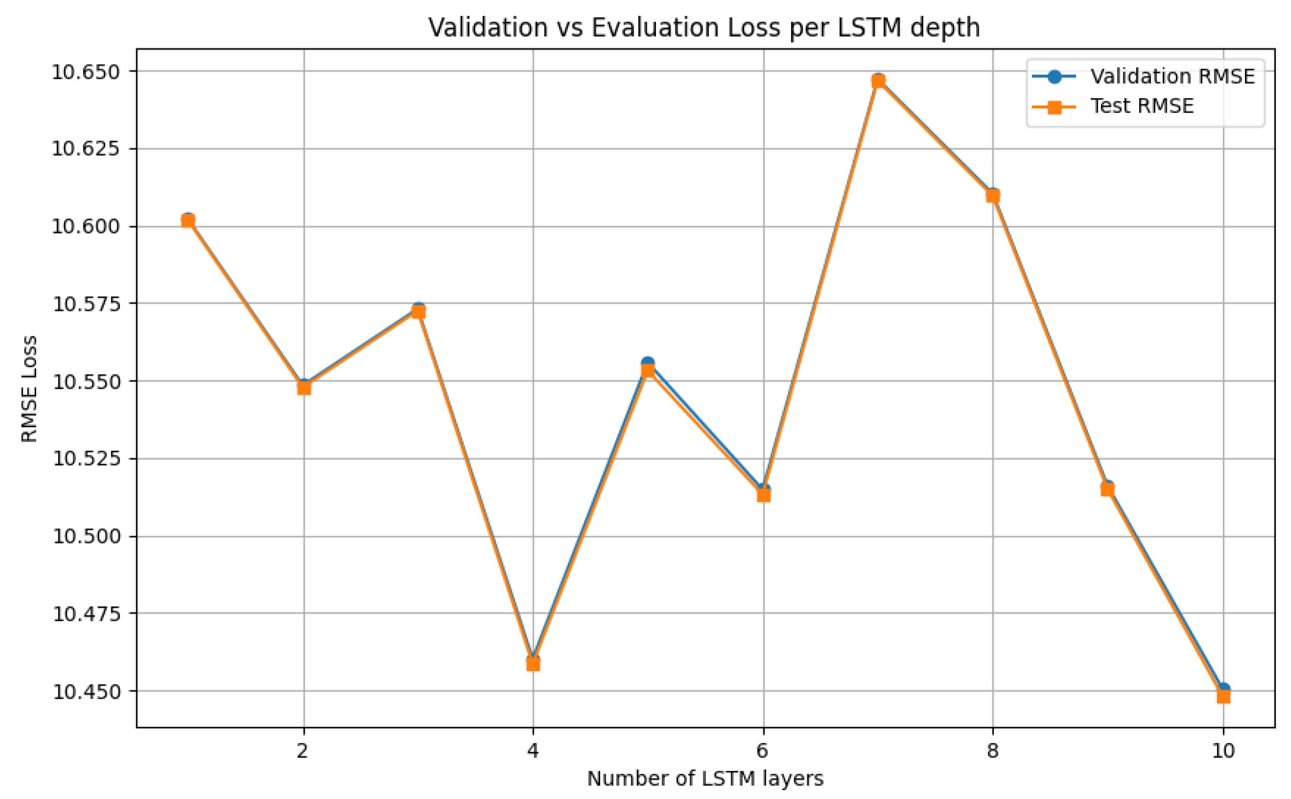
The V-LSTM model hyperparameters auto-tuning step has been performed using the fuzzy encoded dataset, first using the number of cells as a tuning parameter on a minimal of a one LSTM layer architecture, and testing inter-cells distance of ten randomly selected cell cases (unique cells random process) set to 32. The minimum cell value is 32, and the maximum is 512 cells. The portion of the dataset used to validate the models was the of the original dataset. The configuration of the RMSE loss function and the final validation loss at 10 training epochs have been examined for the minimal loss value cells. Figure 10 shows the RMSE loss over the number of cells per layer of the LSTM layer models examined.
From the cell tunning results, the =64 cells/layer achieved the minimum loss of 10.53 for 10 training epochs, followed by the 480 cells/layer model of 10.53. Therefore, the number of 64 cells per layer has been automatically selected by the V-LSTM model. Next, the LSTM layer’s depth is tuned. The tested LSTM models included a variable layer depth starting from 1–10 layers with a layer step of 10 and a random unique selection of 10 models to test. The portion of the dataset used to validate the models was the of the original dataset. The configuration of the RMSE loss function and the final validation loss at 10 training epochs have been examined for the minimal loss value layers.
Figure 11.
V-LSTM model tuning process of the number of model layers using the RMSE as loss function
Figure 11.
V-LSTM model tuning process of the number of model layers using the RMSE as loss function
The LSTM layer tunning process indicated the minimum loss =10, corresponding to the maximum number of testing layers, followed closely by =4. by an RMSE loss difference of 0.01. The authors also noticed that for portions of the dataset and a few epochs, the maximum number of layers always superseded all others, even at a minimal amount. Therefore, for the sake of reducing significantly the number of trainable parameters, they considered a penalty threshold expressed as the min-max loss value multiplied by the min-max weight expression of the number of layers l:
However, in this case, the value was used instead of the value, and the l=10 layers were selected for the number of layers of the V-LSTM model. Table 5 shows the training parameters of the V-LSTM model. Two additional mechanisms are used: 1) An early stop mechanism that ends training when there is no improvement in validation losses for more than five epochs (Early stopping patience) with a min_delta value of , and 2) An adaptive learning rate factor that reduces default learning rate value of using a 25% reduction factor down to , with a patience parameter set to 1 epoch.
During training, the V-LSTM model the selected input temporal depth temporal measurements of the k=6 sensory attribute data together have been transformed into a 2D array of consecutive fermentation parameters.This array corresponds to the previous 24h 5min vectors of measurements of ,pH,T,,, and attributes. Upon data loading, the entire dataset is transformed into batches of (288,6) arrays. These inputs are processed through the first V-LSTM LSTM layer of pre-selected 64 cells out of four layers. The number 64 was chosen during hyperparameters tuning because it maintained the lowest RMSE value (see Figure 10).
4.3.2. V-LSTM Evaluation Results
V-LSTM model training validation and evaluation results are presented in Figure 12, using the RMSE metric, while Table 6 summarizes the results. Initially, the experiment starts training on dataset-1 using the system’s GPU, maintaining a 7.2GB of mean memory utilization during host-to-device transfers. Since an early stop mechanism is used, the number of training epochs per dataset varies. Figure 12a shows the achieved validation loss at the epoch end of each training dataset. Table 6 shows the number of epochs per dataset prior to an early stop if validation loss does not change for more than five epochs, as well as the total mean validation loss achieved by the V-LSTM prediction model. The validation RMSE is relatively low, suggesting the model learns well from the data. The minimal standard deviation indicates consistent performance across training folds, a strong sign of model stability.
Similarly, Figure 12a shows the mean evaluation RMSE loss achieved by the model. The 20% of the total dataset has been used for that purpose and evaluated using 24 core x86 CPU and 32GB of the system RAM. Evaluation loss varies between 0.1578–0.1610 over the trainable datasets, and its value at the training end of the last dataset (d12) was 0.1605. The mean RMSE achieved by the model was 0.1599. The evaluation RMSE is slightly lower than the validation RMSE. This indicates that the model does not overfit and generalizes well to unseen data. The even smaller standard deviation further confirms the model’s fair stability. Since the average number of epochs is around 41 (see Table 6), it is also an indication that the model was not overtrained and converged relatively quickly (41/100 epochs).
Three studies have been used to evaluate our V-LSTM predictor RMSE outputs. The first involves a classifier implemented using input sugar concentrations and alcohol degrees (alcohol concentrations) to predict fermentation behaviors over the first 72h of the fermentation process [65]. This proposed model used two hidden NN layers that are only as big as the bottom part of our proposed V-LSTM predictor and achieved an accuracy of 80% in detecting normal and problematic fermentations using only one parameter as a predictor variable (alcoholic degrees), also denoting the importance of a dense number of samples to achieve significant accuracy results. From the above paper, the authors can only conclude that from the accuracies of this scale, the MSE loss parameters are significantly high and usually above 1.
The second study includes SVR modeling with a Gaussian kernel to predict pH values and Sugar content (measured in Brix) of fermenting wines has shown least RMSE values achieved of 0.142 for pH and 0.804 for Sugar content, giving a least RMSE mean value of 0.473 [66]. This result is 45% more than the loss results our proposed V-LSTM model achieved.
Finally, the last study also includes an NN model [60] of one hidden layer of up to 12 neurons to predict one of the fermentation measurements (preferably alcohol) having the other as model input (pH, CO2, , ), that achieved a minimum MSE value of 0.99 which corresponds to an RMSE of 0.995, that is 73.74% more than the achieved RMSE values of the V-LSTM model.
5. Conclusions
This paper presents a new wine fermentation monitoring system called SmartBarrel. The system is equipped with two low-cost probing IoT devices, an Electronic nose capable of monitoring fermenting gas releases of alcohol, CO, and CO2, and an electronic tongue capable of monitoring basic wine fermenting parameters such as fermentation residues, pH, sugar concentrations and color changes. These IoT devices are installed on the lid of stainless steel fermentation tanks, probing and transmitting close to real-time measurements to the cloud. The system is assisted by the community edition open-source ThingBoard AS platform and ThingsBoard mobile application for remote monitoring and visualization. The proposed system supports cloud services and visualization and utilizes the Cassandra NoSQL database for its data storage location.
The authors also added the capability in their SmartBarrel system to offer a real-time estimation of alcohol degrees without using an additional meter but with a fuzzy controller capable of inferring alcoholic content from fermentation parameters. This fuzzy controller can also be implemented at the IoT device level. The authors also proposed a cloud-based variable cells and layers LSTM model called V-LSTM for predicting future fermentation parameters trained on either past fermentation data or data provided by fuzzy logic autoencoders. The proposed VLTM model can also auto-tune its model schema of the number of LSTM layers and cells per layer used based on portions of data training and, therefore, selecting the best hyperparameters per case study or scenario. The authors set as future work a modification of their currently proposed VLSTM model that can have multiple strands [36], due to the selection of different hyperparameter values on re-training on new data, and therefore policies to apply the best strand inferences for each case accordingly.
The authors’ experimentation focused mainly on the E-nose SmartBarrel node, validating its functionality and overall SmartBarrel system functionality via the alcohol fuzzy controller inferences, achieving an score of 0.87 over new SmartBarrel fermentation data. Furthermore, the authors also experimented with their proposed V-LSTM predictor, showing that it can achieve RMSE scores down to 0.16, which is 45-73% less than existing prediction SVR and shallow NN models. The authors also denote the need for a dense-cloud-based measurement of wine fermenting parameters for deep learning models such as V-LSTM to achieve even better prediction results.
Author Contributions
Conceptualization, S.K.; methodology, S.K.; software, S.K.; validation, M.T.; formal analysis, M.T. and Y.K.; investigation, S.K.; resources, S.K.; data curation, M.T.; writing—original draft preparation, S.K and G.K.; writing—review and editing, C.P. and G.K.; visualization, S.K.; supervision, C.P. and Y.K.; project administration, S.K. The author has read and agreed to the published version of the manuscript.
Funding
This research received no external funding
Institutional Review Board Statement
Not Applicable
Informed Consent Statement
Not Applicable
Data Availability Statement
No new data were created
Conflicts of Interest
The author declares no conflict of interest.
Abbreviations
The following abbreviations are used in this manuscript:
| AS | Application Server |
| CNN | Convolutional Neural Network |
| CPU | Central Processing Unit |
| DL | Deep Learning |
| DSS | Decision Support System |
| LSTM | Long short-term memory RNN |
| ML | Machine Learning |
| MOS | Metal Oxide Semiconductor |
| NDIR | Non-Dispersive Infrared |
| NIR | Near Infrared Region of wavelength between 750 nm to 2500 nm |
| NN | Neural Networks |
| P-Eye | Probing Eye |
| P-Nose | Probing Nose |
| P-Tongue | Probing Tongue |
| RNN | Recurrent Neural Networks |
| SVR | Support Vector Regression |
| V-LSTM | LSTM of variable cells and layers |
| VM | Virtual Machines, cloud hosted |
References
- Gallego-Martinez, J.J.; Canete-Carmona, E.; Gersnoviez, A.; Brox, M.; Sánchez-Gil, J.J.; Martín-Fernández, C.; Moreno, J. Devices for monitoring oenological processes: A review. Measurement 2024, 235, 114922. [Google Scholar] [CrossRef]
- Sainz, B.; Antolín, J.; López-Coronado, M.; Castro, C.D. A Novel Low-Cost Sensor Prototype for Monitoring Temperature during Wine Fermentation in Tanks. Sensors 2013, 13, 2848–2861. [Google Scholar] [CrossRef] [PubMed]
- Naveed, M. The Adoption of 4.0 Agriculture for Wine Production in Order to Improve Efficiency, Sustainability and Competitiveness. Technical report, Universita degli Studi di Foggia, 2024. Accepted: 2024-11-20T03:10:06Z Publisher: Universita degli Studi di Foggia.
- Karaiskos, V.; Zinas, N.; Gkamas, T.; Karolos, I.; Pikridas, C.; Vrettos, N.; Tsioukas, V.; Kontogiannis, S. Proposed Industry 4.0 Maintenance Framework for Critical and Demanding Infrastructures and Processes. In Proceedings of the Proc. of the 7th South-East Europe Design Automation, Computer Engineering, Computer Networks and Social Media Conference (SEEDA-CECNSM), 2022, pp. 1–5. [CrossRef]
- Asiminidis, C.; Kokkonis, G.; Kontogiannis, S. Managing IoT data using relational schema and JSON fields, a comparative study. IOSR Journal of Computer Engineering (IOSR-JCE) 2018, 20, 46–52. [Google Scholar]
- Asiminidis, C.; Kokkonis, G.; Kontogiannis, S. Database Systems Performance Evaluation for IoT Applications. International Journal of Database Management Systems (IJDMS) 2018, 10. [Google Scholar] [CrossRef]
- Cao, J. AI: A New and Impactful Player in the Quality Evaluation of Wine. Harvard Data Science Review 2025, 7. [Google Scholar] [CrossRef]
- Dewan, A.; Nagaraja, S.K.; Yadav, S.; Bishnoi, P.; Malik, M.; Chhikara, N.; Luthra, A.; Singh, A.; Davis, C. ; Poonam. Advances in Wine Processing: Current Insights, Prospects, and Technological Interventions. Food and Bioprocess Technology, 2025. [Google Scholar] [CrossRef]
- Kontogiannis, S.; Asiminidis, C. A Proposed Low-Cost Viticulture Stress Framework for Table Grape Varieties. IoT 2020, 1, 337–359. [Google Scholar] [CrossRef]
- Ammoniaci, M.; Kartsiotis, S.P.; Perria, R.; Storchi, P. State of the Art of Monitoring Technologies and Data Processing for Precision Viticulture. Agriculture 2021, 11, 201. [Google Scholar] [CrossRef]
- Kontogiannis, S.; Konstantinidou, M.; Tsioukas, V.; Pikridas, C. A Cloud-Based Deep Learning Framework for Downy Mildew Detection in Viticulture Using Real-Time Image Acquisition from Embedded Devices and Drones. Information 2024, 15. [Google Scholar] [CrossRef]
- Kontogiannis, S.; Koundouras, S.; Pikridas, C. Proposed Fuzzy-Stranded-Neural Network Model That Utilizes IoT Plant-Level Sensory Monitoring and Distributed Services for the Early Detection of Downy Mildew in Viticulture. Computers 2024, 13, 63. [Google Scholar] [CrossRef]
- Li, B.; Wang, J.; Zhang, R. Detection and analysis of electrochemical signals in wine fermentation process. Journal of Food Measurement and Characterization 2023, 17. [Google Scholar] [CrossRef]
- Bender, M.; Kirdan, E.; Pahl, M.O.; Carle, G. Open-Source MQTT Evaluation. In Proceedings of the IEEE 18th Annual Consumer Communications and Networking Conference(CCNC); 2021; Vol. 1, pp. 1–4. [Google Scholar] [CrossRef]
- Gonçalves, F.; Oliveira, N.; Duarte, D.P.; Nogueira, R.N. WinePlus 1110: The Remote and Real-Time Wine Fermentation Process Monitoring System. In Proceedings of the Conference Proceedings, July 2019. Accessed: 2025-05-04.
- Chiou, C.W.; Huang, S.Z.; Sun, Y.S. A Mobile Control System of Fermentation Temperature on Winemaking. International Journal of Food Science and Agriculture 2022, 6. [Google Scholar] [CrossRef]
- Nelson, J.; Boulton, R.; Knoesen, A. Automated Density Measurement With Real-Time Predictive Modeling of Wine Fermentations. IEEE Transactions on Instrumentation and Measurement 2022, 71, 1–7. [Google Scholar] [CrossRef]
- Masetti, G.; Marazzi, F.; Di Cecilia, L.; Rovati, L. IOT-Based Measurement System for Wine Industry. In Proceedings of the 2018 Workshop on Metrology for Industry 4.0 and IoT, Apr 2018, pp. 163–168. [CrossRef]
- Angelkov, D.; Martinovska Bande, C. Sensor Module for Monitoring Wine Fermentation Process. In Proceedings of the Applied Physics, System Science and Computers; Ntalianis, K.; Croitoru, A., Eds., Cham, 2018; pp. 253–262. [CrossRef]
- Vasilescu, A.; Fanjul-Bolado, P.; Titoiu, A.M.; Porumb, R.; Epure, P. Progress in Electrochemical (Bio)Sensors for Monitoring Wine Production. Chemosensors 2019, 7, 66. [Google Scholar] [CrossRef]
- Nanou, E.; Mavridou, E.; Milienos, F.; Papadopoulos, G.; Tempère, S.; Kotseridis, Y. Odor Characterization of White Wines Produced from Indigenous Greek Grape Varieties Using the Frequency of Attribute Citation Method with Trained Assessors. Foods 2020, 9, 1396. [Google Scholar] [CrossRef] [PubMed]
- Kontogiannatos, D.; Troianou, V.; Dimopoulou, M.; Hatzopoulos, P.; Kotseridis, Y. Oenological Potential of Autochthonous Saccharomyces cerevisiae Yeast Strains from the Greek Varieties of Agiorgitiko and Moschofilero. Beverages 2021, 7, 27. [Google Scholar] [CrossRef]
- Niyigaba, T.; Küçükgöz, K.; Kołożyn-Krajewska, D.; Królikowski, T.; Trząskowska, M. Advances in Fermentation Technology: A Focus on Health and Safety. Applied Sciences 2025, 15, 3001. [Google Scholar] [CrossRef]
- Izquierdo-Bueno, I.; Moraga, J.; Cantoral, J.M.; Carbú, M.; Garrido, C.; González-Rodríguez, V.E. Smart Viniculture: Applying Artificial Intelligence for Improved Winemaking and Risk Management. Applied Sciences 2024, 14, 10277. [Google Scholar] [CrossRef]
- Alfieri, G.; Modesti, M.; Riggi, R.; Bellincontro, A. Recent Advances and Future Perspectives in the E-Nose Technologies Addressed to the Wine Industry. Sensors 2024, 24, 2293. [Google Scholar] [CrossRef]
- Munoz-Castells, R.; Modesti, M.; Moreno-Garcia, J.; Rodriguez-Moreno, M.; Catini, A.; Capuano, R.; Di Natale, C.; Bellincontro, A.; Moreno, J. Differentiation through E-nose and GC-FID data modeling of rosé sparkling wines elaborated via traditional and Charmat methods. Journal of the Science of Food and Agriculture 2025, 105, 1439–1447. [Google Scholar] [CrossRef]
- Summerson, V.; Gonzalez Viejo, C.; Pang, A.; Torrico, D.D.; Fuentes, S. Assessment of Volatile Aromatic Compounds in Smoke Tainted Cabernet Sauvignon Wines Using a Low-Cost E-Nose and Machine Learning Modelling. Molecules 2021, 26, 5108. [Google Scholar] [CrossRef]
- Shahid, A.; Choi, J.H.; Rana, A.; Kim, H.S. Least Squares Neural Network-Based Wireless E-Nose System Using an SnO2 Sensor Array. Sensors 2018, 18, 1446. [Google Scholar] [CrossRef]
- Buratti, S.; Benedetti, S. Chapter 28 - Alcoholic Fermentation Using Electronic Nose and Electronic Tongue. In Electronic Noses and Tongue. In Electronic Noses and Tongues in Food Science; Rodríguez Méndez, M.L., Ed.; Academic Press: San Diego, 2016; pp. 291–299. [Google Scholar] [CrossRef]
- Tomtsis, D.; Kontogiannis, S.; Kokkonis, G.; Zinas, N. IoT Architecture for Monitoring Wine Fermentation Process of Debina Variety Semi-Sparkling Wine. In Proceedings of the Proceedings of the SouthEast European Design Automation, Computer Engineering, Computer Networks and Social Media Conference, New York, NY, USA, Jun 2016; SEEDA-CECNSM ’16, pp. 42–47. [CrossRef]
- Littarru, E.; Modesti, M.; Alfieri, G.; Pettinelli, S.; Floridia, G.; Bellincontro, A.; Sanmartin, C.; Brizzolara, S. Optimizing the winemaking process: NIR spectroscopy and e-nose analysis for the online monitoring of fermentation. Journal of the Science of Food and Agriculture 2025, 105, 1465–1475. [Google Scholar] [CrossRef] [PubMed]
- Modesti, M.; Alfieri, G.; Pardini, L.; Cerreta, R.; Mencarelli, F.; Bellincontro, A. Application of a Low-Cost Device VIS-NIRs-Based for Polyphenol Monitoring During the Vinification Process. IVES Conference Series 2022. Accessed: 2025-05-04.
- Taglieri, I.; Mencarelli, F.; Bellincontro, A.; Modesti, M.; Cerreta, R.; Zinnai, A. Development of a micro-Vis-NIR and SAW Nanobiosensor to Measure Polyphenols in Must/Wine On-Time and Online. Acta Horticulturae 2023, 1370, 39–46. [Google Scholar] [CrossRef]
- Cozzolino, D.; Kwiatkowski, M.J.; Parker, M.; Cynkar, W.U.; Dambergs, R.G.; Gishen, M.; Herderich, M.J. Prediction of phenolic compounds in red wine fermentations by visible and near infrared spectroscopy. Analytica Chimica Acta 2004, 513, 73–80. [Google Scholar] [CrossRef]
- Kontogiannis, S.; Gkamas, T.; Pikridas, C. Deep Learning Stranded Neural Network Model for the Detection of Sensory Triggered Events. Algorithms 2023, 16, 202. [Google Scholar] [CrossRef]
- Kontogiannis, S.; Kokkonis, G.; Pikridas, C. Proposed Long Short-Term Memory Model Utilizing Multiple Strands for Enhanced Forecasting and Classification of Sensory Measurements. Mathematics 2025, 13, 1263. [Google Scholar] [CrossRef]
- Kontogiannis, S.; Kokkonis, G. Proposed Fuzzy Real-Time HaPticS Protocol Carrying Haptic Data and Multisensory Streams. INTERNATIONAL JOURNAL OF COMPUTERS COMMUNICATIONS & CONTROL 2020, 15. [Google Scholar]
- Kontogiannis, S.; Kokkonis, G.; Ellinidou, S.; Valsamidis, S. Proposed Fuzzy-NN Algorithm with LoRaCommunication Protocol for Clustered Irrigation Systems. Future Internet 2017, 9, 78. [Google Scholar] [CrossRef]
- Kokkonis, G.; Chatzimparmpas, A.; Kontogiannis, S. Middleware IoT protocols performance evaluation for carrying out clustered data. In Proceedings of the South-Eastern European Design Automation, Computer Engineering, Computer Networks and Society Media Conference (SEEDA CECNSM), 2018, Vol. 1, pp. 1–5. [CrossRef]
- ThingsBoard. ThingsBoard Open-source IoT Platform, 2019. Available at: https://thingsboard.io/, [Online; accessed Oct 2020].
- Seesaard, T.; Wongchoosuk, C. Recent Progress in Electronic Noses for Fermented Foods and Beverages Applications. Fermentation 2022, 8, 302. [Google Scholar] [CrossRef]
- Oikonomou, P.; Goustouridis, D.; Raptis, I.; Manoli, K.; Sanopoulou, M. Must fermentation progress monitoring by polymer coated capacitive vapour sensor arrays. In Proceedings of the SENSORS, 2009 IEEE, 2009, pp. 1443–1446. [CrossRef]
- Canete-Carmona, E.; Gallego-Martinez, J.J.; Martin, C.; Brox, M.; Luna-Rodriguez, J.J.; Moreno, J. A Low-Cost IoT Device to Monitor in Real-Time Wine Alcoholic Fermentation Evolution Through CO2 Emissions. IEEE Sensors Journal 2020, 20, 6692–6700. [Google Scholar] [CrossRef]
- Ye, M.; Liu, Y.; Li, Q. Recent Progress in Smart Electronic Nose Technologies Enabled with Machine Learning Methods. Sensors 2021, 21, 7620. [Google Scholar] [CrossRef] [PubMed]
- Lozano, J.; Santos, J.; Horrillo, M. Wine Applications With Electronic Noses. In Electronic Noses and Tongues in Food Science; Méndez, M.L.R., Ed.; Academic Press, 2016; pp. 137–148. [CrossRef]
- Vanaraj, R.; I. P, B.; Mayakrishnan, G.; Kim, I.S.; Kim, S.C. A Systematic Review of the Applications of Electronic Nose and Electronic Tongue in Food Quality Assessment and Safety. Chemosensors 2025, 13, 161. [CrossRef]
- Peris, M.; Escuder-Gilabert, L. On-line Monitoring of Food Fermentation Processes Using Electronic Noses and Electronic Tongues: A Review. Analytica Chimica Acta 2013, 804, 29–36. [Google Scholar] [CrossRef]
- Syahputra, T.S.; Ihsan, N.; Kombo, K.O.; Faizah, K.; Wahyono.; Widada, J.; Triyana, K. Integration of low-cost multispectral sensors and electronic nose for enhanced fermentation monitoring in tempeh production. Journal of Food Measurement and Characterization 2025, 19, 3687–3701. [CrossRef]
- Sun, H.; Ma, H.; Hao, M.; Pretorius, I.S.; Chen, S. Identification of yeast population dynamics of spontaneous fermentation in Beijing wine region, China. Annals of Microbiology 2009, 59, 69–76. [Google Scholar] [CrossRef]
- Li, C.; Wang, Y.; Sha, S.; Yin, H.; Zhang, H.; Wang, Y.; Zhao, B.; Song, F. Analysis of the tendency for the electronic conductivity to change during alcoholic fermentation. Scientific Reports 2019, 9, 5512. [Google Scholar] [CrossRef]
- Han, F.; Zhang, D.; Aheto, J.; Feng, F.; Duan, T. Integration of a Low-Cost Electronic Nose and a Voltammetric Electronic Tongue for Red Wines Identification. Journal of Food Science & Nutrition 2020, 8, 4330–4339. [Google Scholar] [CrossRef]
- Martelo-Vidal, M.J.; Vázquez, M. Determination of polyphenolic compounds of red wines by UV-VIS-NIR spectroscopy and chemometrics tools. Food Chemistry 2014, 158, 28–34. [Google Scholar] [CrossRef]
- Jeong, J.; Kim, S. Application of machine learning for quantitative analysis of industrial fermentation using image processing. Food Science and Biotechnology 2025, 34, 373–381. [Google Scholar] [CrossRef]
- Cheynier, V.; Dueñas-Paton, M.; Salas, E.; Maury, C.; Souquet, J.M.; Sarni-Manchado, P.; Fulcrand, H. Structure and Properties of Wine Pigments and Tannins. American Journal of Enology and Viticulture 2006, 57, 298. [Google Scholar] [CrossRef]
- Nel, A.P. Tannins and anthocyanins: From their origin to wine analysis - A review. South African Journal of Enology and Viticulture 2018, 39, 1–20. [Google Scholar] [CrossRef]
- Figueiredo-González, M.; Cancho-Grande, B.; Simal-Gándara, J. Effects on colour and phenolic composition of sugar concentration processes in dried-on- or dried-off-vine grapes and their aged or not natural sweet wines. Trends in Food Science & Technology 2013, 31, 36–54. [Google Scholar] [CrossRef]
- Goode, J. Flawless: Understanding Faults in Wine; Univ of California Press, 2018.
- Cosme, F.; Nunes, F.M.; Filipe-Ribeiro, L. Chemistry and Biochemistry of Winemaking, Wine Stabilization and Aging; BoD – Books on Demand, 2021.
- Gkamas, T.; Karaiskos, V.; Kontogiannis, S. Performance Evaluation of Distributed Database Strategies Using Docker as a Service for Industrial IoT Data: Application to Industry 4.0. Information 2022, 13, 190. [Google Scholar] [CrossRef]
- Sipos, A.; Florea, A.; Arsin, M.; Fiore, U. Using Neural Networks to Obtain Indirect Information about the State Variables in an Alcoholic Fermentation Process. Processes 2021, 1, 74. [Google Scholar] [CrossRef]
- Oikonomou, P.; Raptis, I.; Sanopoulou, M. Monitoring and Evaluation of Alcoholic Fermentation Processes Using a Chemocapacitor Sensor Array. Sensors 2014, 14, 16258–16273. [Google Scholar] [CrossRef]
- Darias-Martin, J.; Socas-Hernandez, A.; Diaz-Romero, C.; Diaz-Diaz, E. Comparative study of methods for determination of titrable acidity in wine. Journal of Food Composition and Analysis 2003, 16. [Google Scholar] [CrossRef]
- Kaur, N.; Kaur, G.; Aruchamy, P.; Chaudhary, N. An Integrated Approach Based on Fuzzy Logic and Machine Learning Techniques for Reliable Wine Quality Prediction. Procedia Computer Science 2025, 252, 613–622. [Google Scholar] [CrossRef]
- Prusova, B.; Humaj, J.; Kulhankova, M.; Kumsta, M.; Sochor, J.; Baron, M. Capture of Fermentation Gas from Fermentation of Grape Must. Foods 2023, 12, 574. [Google Scholar] [CrossRef]
- Román, R.C.; Hernández, O.G.; Urtubia, U.A. Prediction of problematic wine fermentations using artificial neural networks. Bioprocess and Biosystems Engineering 2011, 34, 1057–1065. [Google Scholar] [CrossRef]
- Silva, R.; Gomes, V.; Mendes-Faia, A.; Melo-Pinto, P. Using Support Vector Regression and Hyperspectral Imaging for the Prediction of Oenological Parameters on Different Vintages and Varieties of Wine Grape Berries. Remote Sensing 2018, 10, 312. [Google Scholar] [CrossRef]
Figure 1.
SmartBarrel High-level system architecture and system components
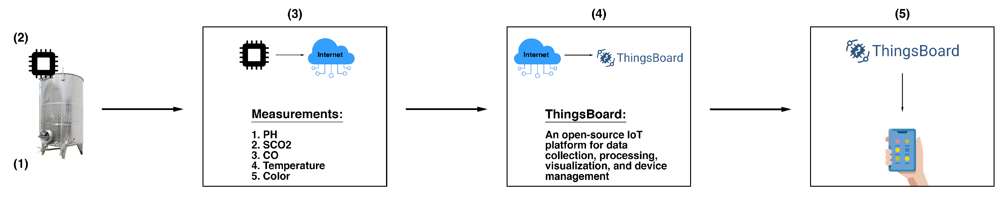
Figure 2.
Illustration of the SmartBarrel E-nose device, parts, and sensory components
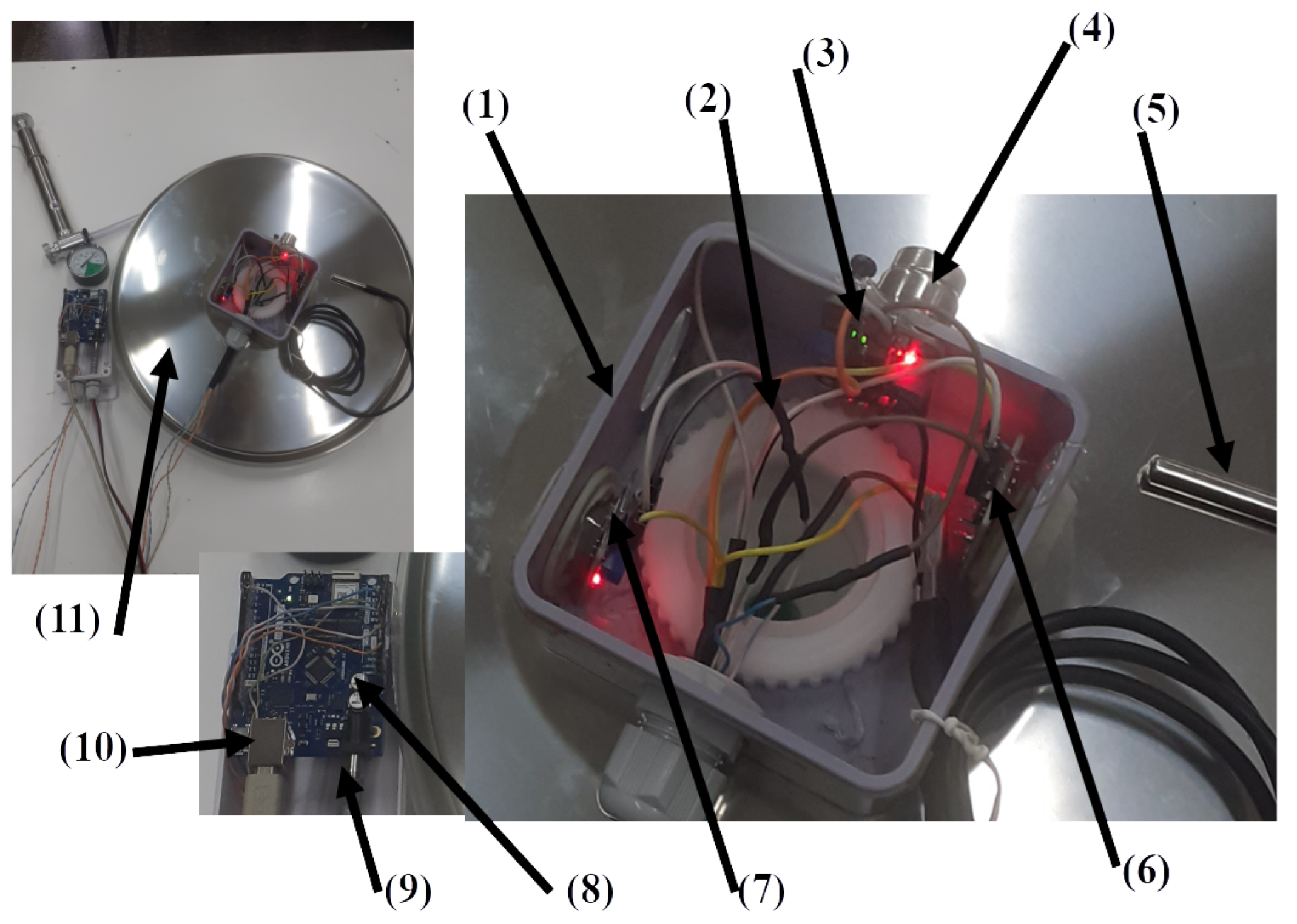
Figure 3.
Illustration of the SmartBarrel E-tongue device, parts, and sensory components
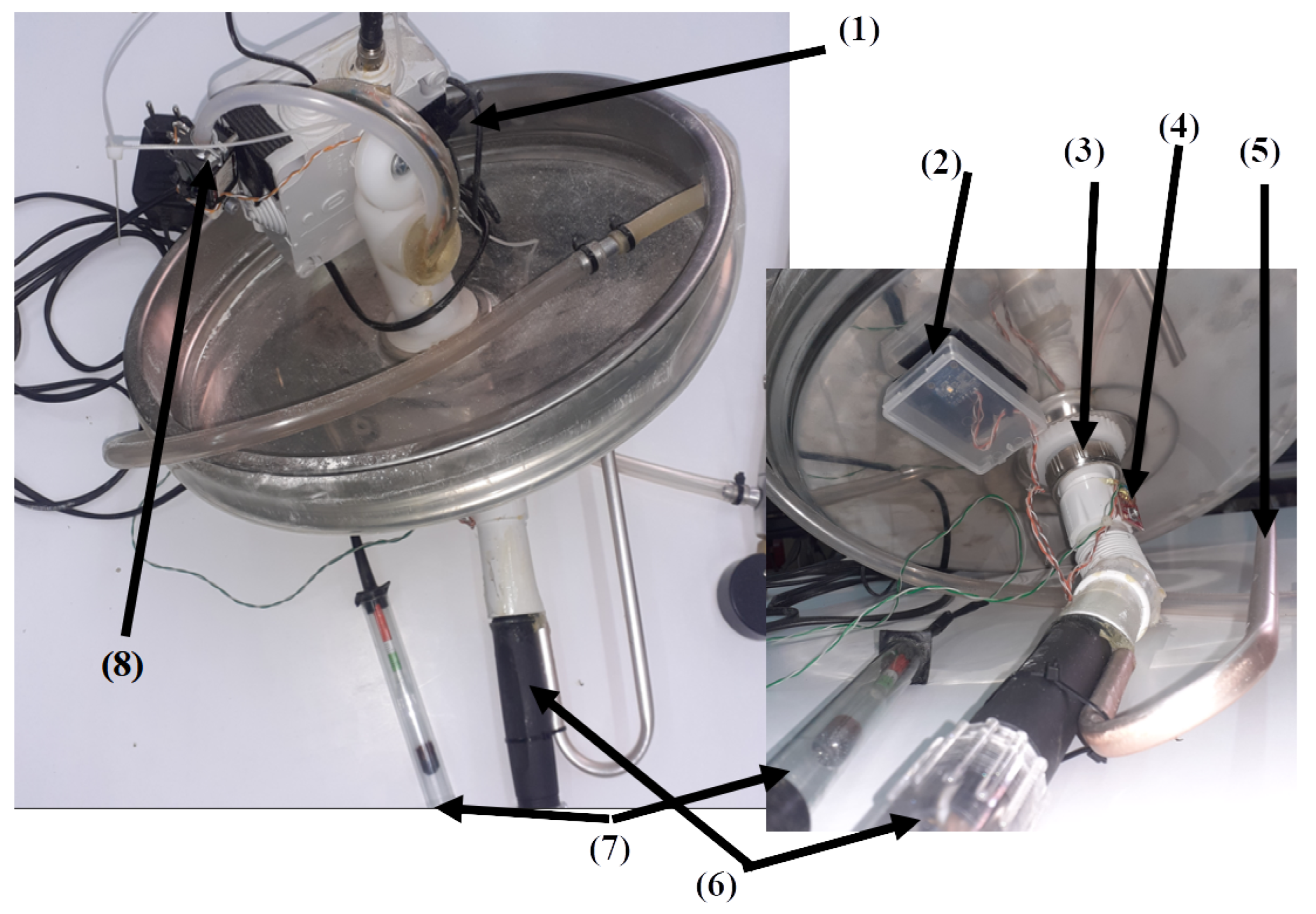
Figure 4.
V-LSTM process flow diagram of fuzzy parameters generation, hyperparameters training, model training and predictions over new data streams
Figure 4.
V-LSTM process flow diagram of fuzzy parameters generation, hyperparameters training, model training and predictions over new data streams
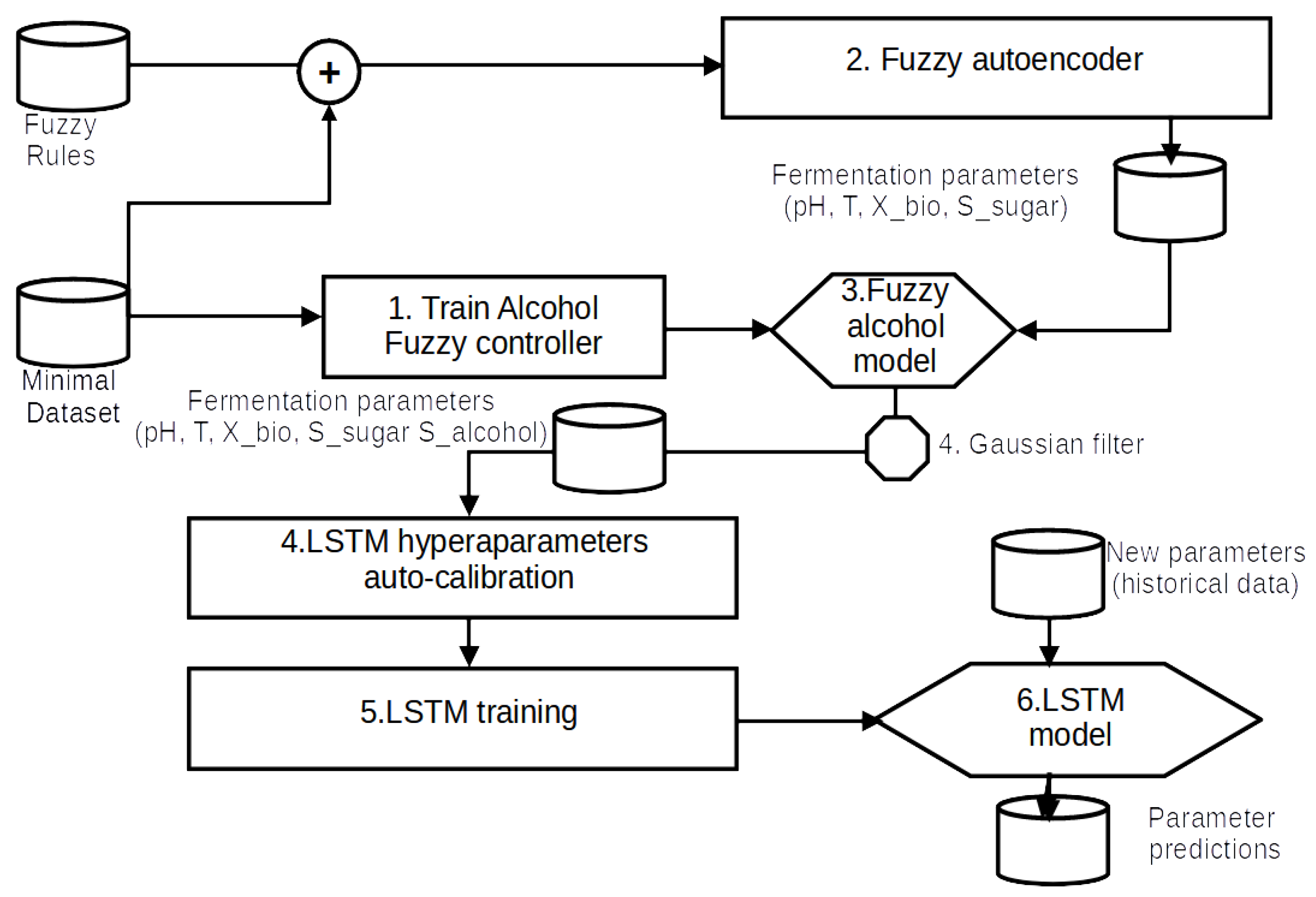
Figure 5.
V-LSTM model structure, layers, data input and output
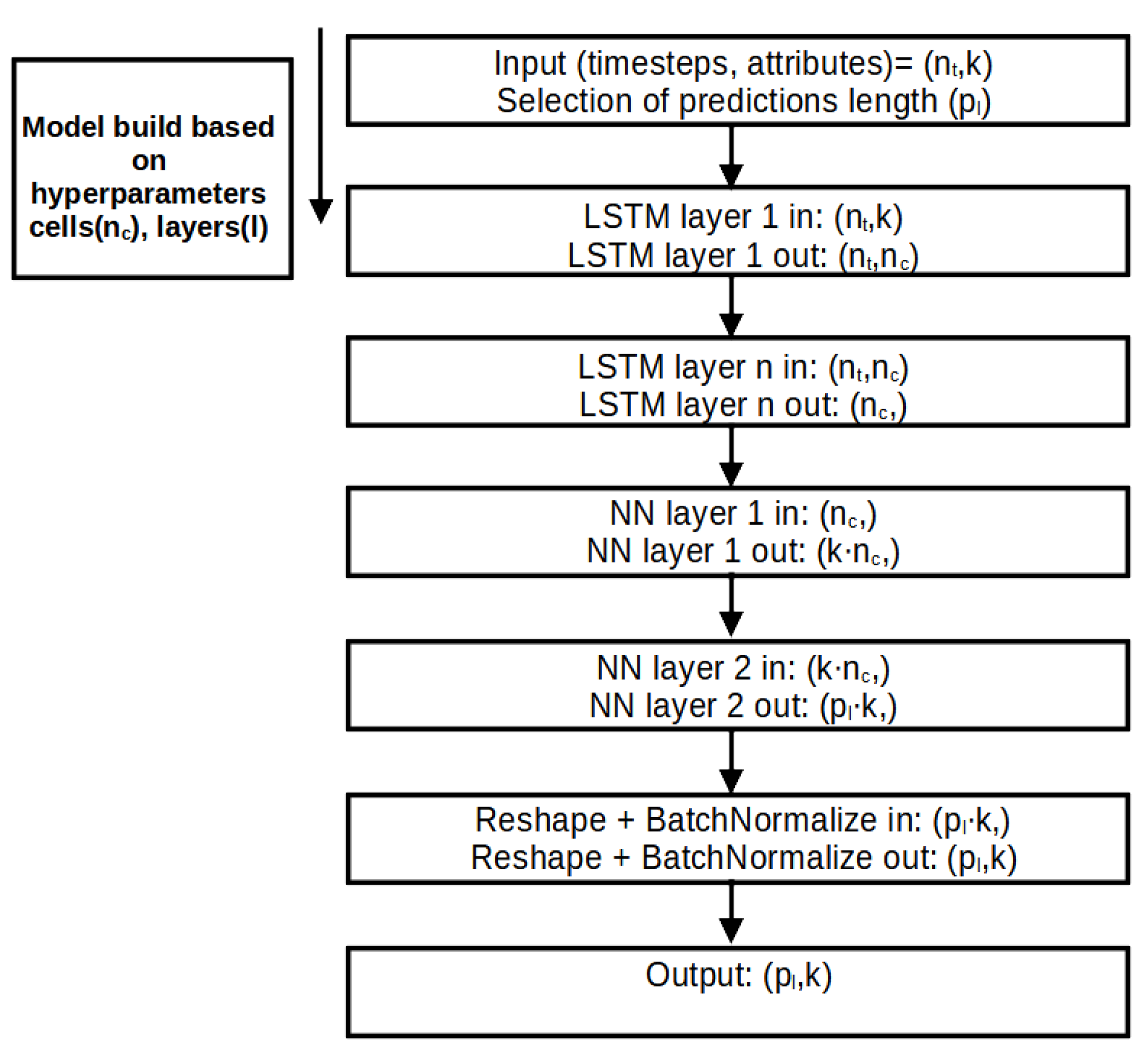
Figure 6.
SmartBarrel E-nose Evaluation for the fermentation of a Debina rose mix of white Debina variety with red Vlachiko variety in the area of Zitsa, Epirus, Greece
Figure 6.
SmartBarrel E-nose Evaluation for the fermentation of a Debina rose mix of white Debina variety with red Vlachiko variety in the area of Zitsa, Epirus, Greece
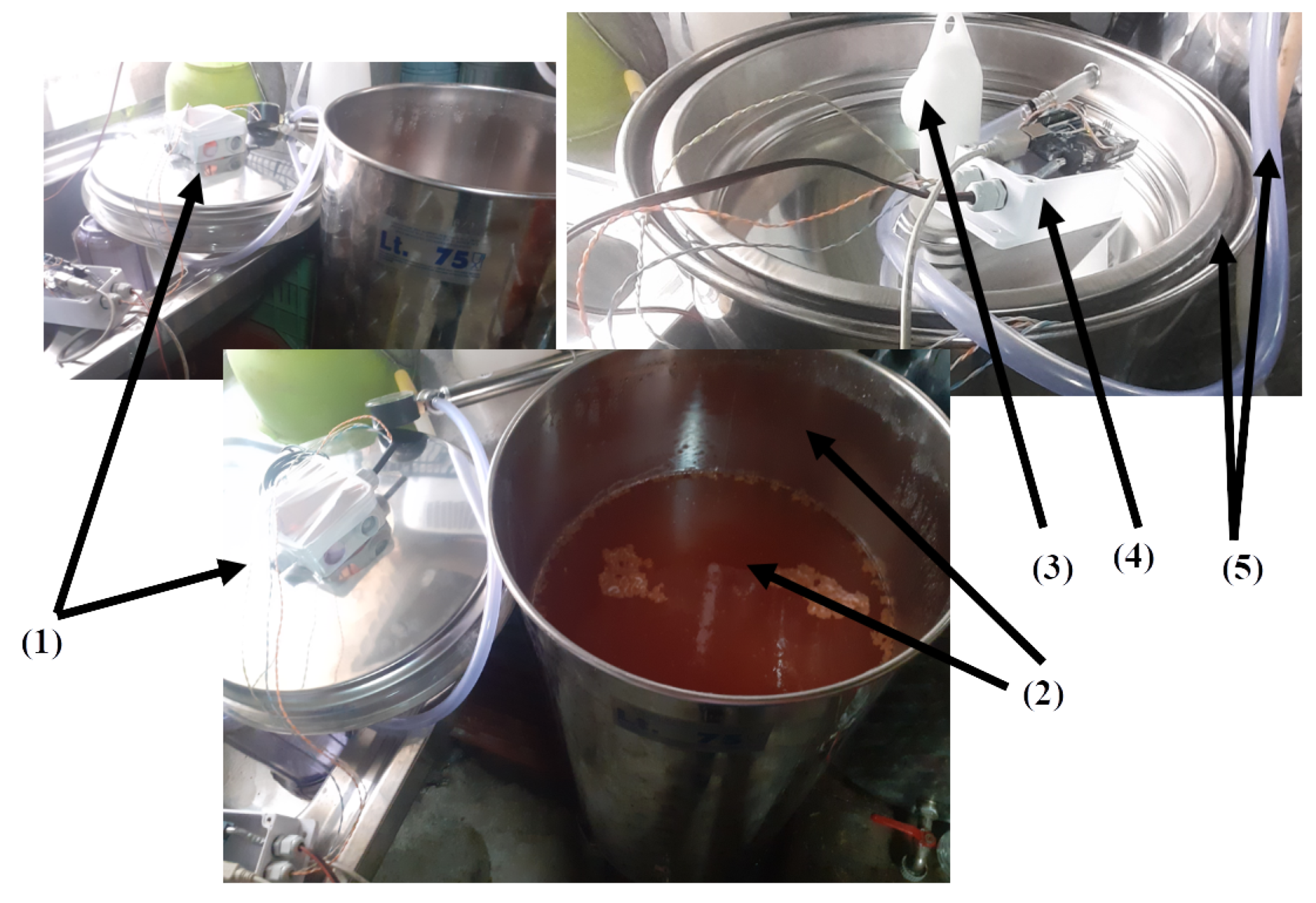
Figure 7.
SmartBarrel E-nose (P-nose) gas concentration measurements from MQ-7 (CO) MOS sensor, MG-811 (CO2) NDIR like solid-state electrochemical sensor, and MQ-3 MOS alcohol sensor, showing both processed concentrations and raw signals. The upper row displays (a) carbon monoxide (CO) and (b) carbon dioxide (CO2) concentrations in parts per million, while the lower row shows (c) ethanol concentrations (C2H5OH) in milligrams per liter and (d) the corresponding raw sensor outputs.
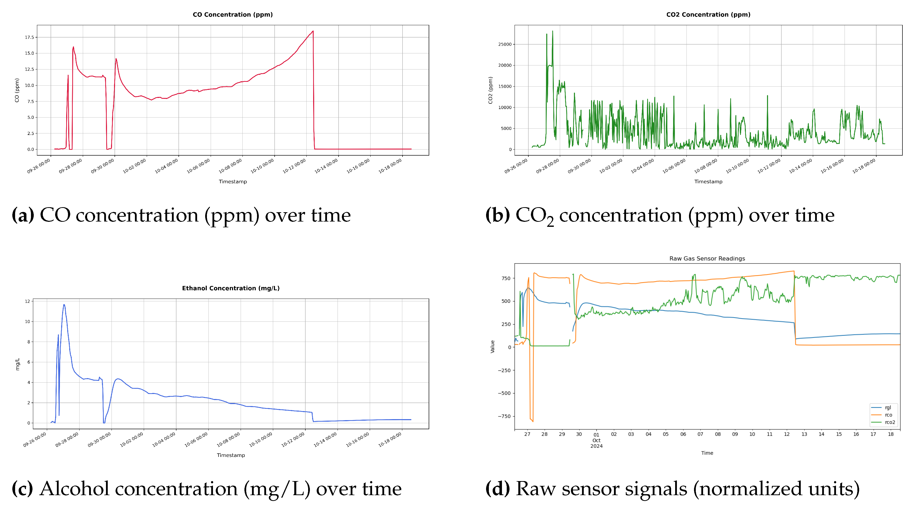
Figure 8.
SmartBarrel E-nose temperature plot in the air and inside the fermenting yeast (internal temperature)
Figure 8.
SmartBarrel E-nose temperature plot in the air and inside the fermenting yeast (internal temperature)
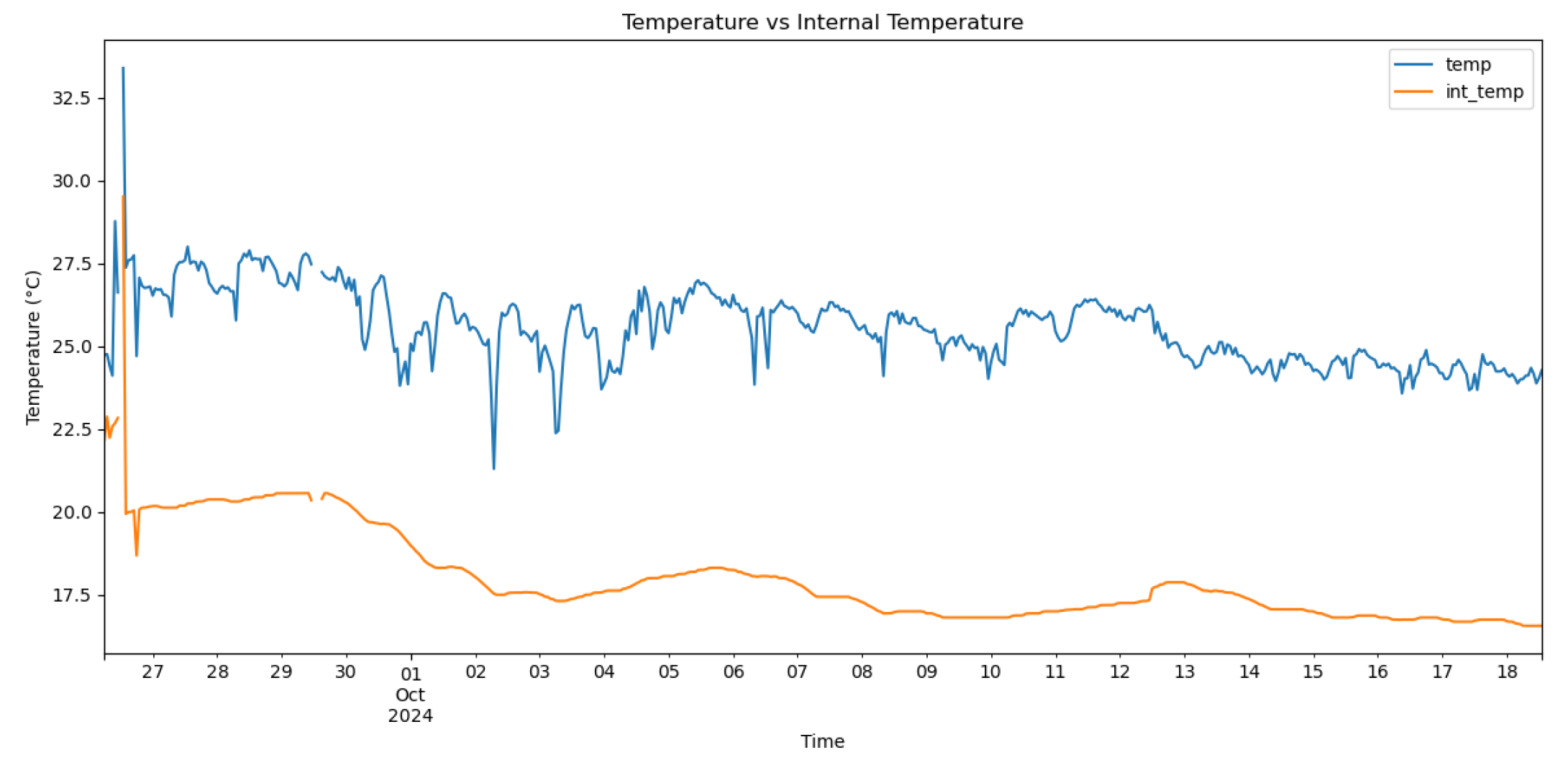
Figure 9.
Alcohol fuzzy controller inference values (green line) over not known fermentation curve of alcohol concentrations (blue line)
Figure 9.
Alcohol fuzzy controller inference values (green line) over not known fermentation curve of alcohol concentrations (blue line)
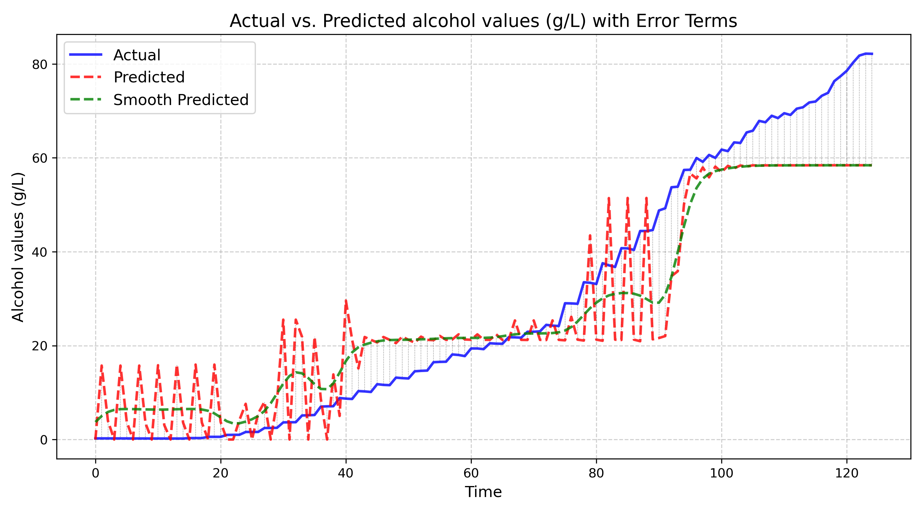
Figure 10.
V-LSTM model tuning process of the number of cells per V-LSTM layer using the RMSE as loss function
Figure 10.
V-LSTM model tuning process of the number of cells per V-LSTM layer using the RMSE as loss function
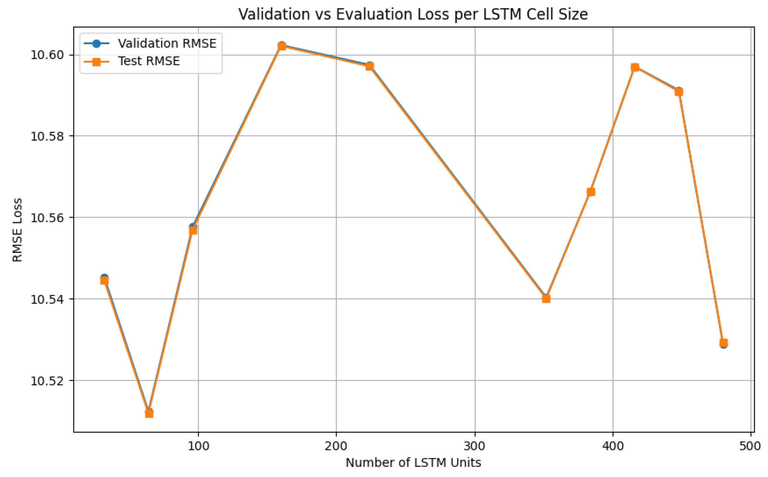
Figure 12.
Validation and evaluation results of the V-LSTM model
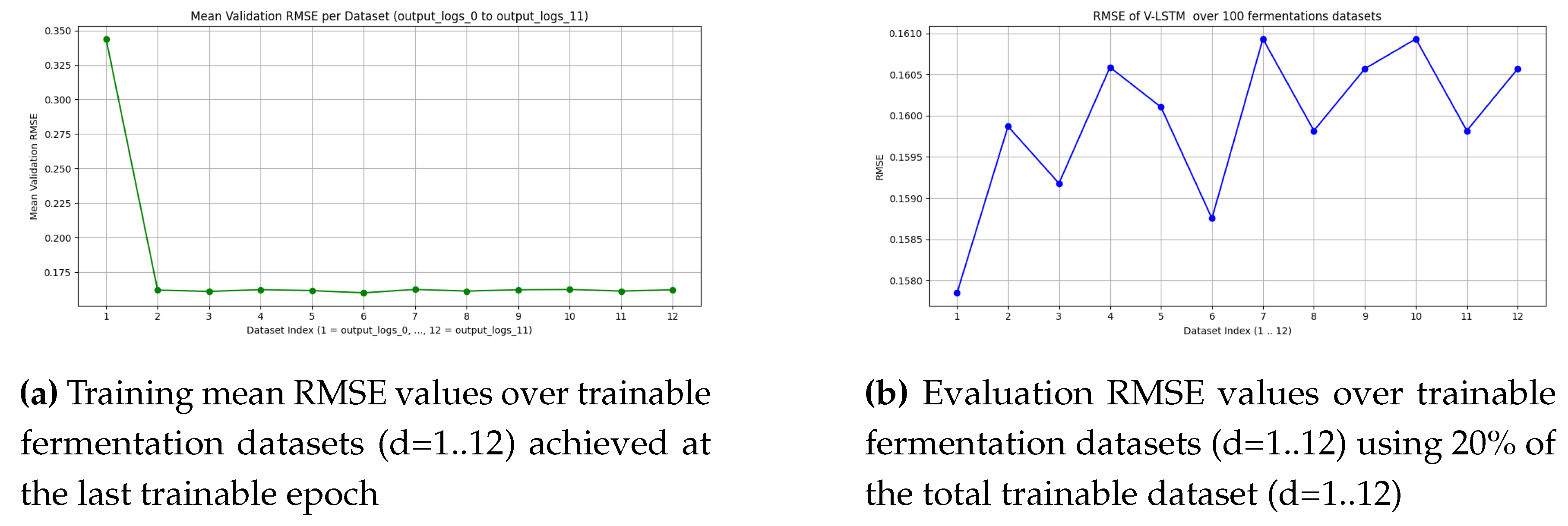

Table 1.
Fuzzy controller that partitions attributes (both antecedents and consequence) into three classes (low, medium, high) with Gaussian MFs hyperparameters and calibrated values to achieve minimum RMSE
Table 1.
Fuzzy controller that partitions attributes (both antecedents and consequence) into three classes (low, medium, high) with Gaussian MFs hyperparameters and calibrated values to achieve minimum RMSE
| Hyperparameter | Description | Calculation | Calibrated Value |
|---|---|---|---|
| offset | offset from minimum value for the attribute | ||
| offset | offset from minimum value for the attribute | ||
| w curve bandwidth | Width of the gaussian-skewed gaussian curve expressed as a fraction of the standard deviation | default k=3 | |
| center value of the low membership function | |||
| center value of the medium membership function | |||
| center value of the high membership function | kd=1 |
Table 2.
Fuzzy Rule Base for Fermentation Phases
| Antecedent | Consequent |
|---|---|
| IF phase is lag | THEN biomass grows slowly (), sugar remains high (210 g/L) |
| IF phase is exponential | THEN biomass follows sigmoid (), sugar decays exponentially |
| IF phase is stationary | THEN biomass declines linearly (), sugar approaches 30 g/L |
| IF phase is death | THEN biomass decays exponentially (), sugar stabilizes at 20 g/L |
| IF phase is lag | THEN pH = 4.5 (constant), C |
| IF phase is exponential | THEN pH decreases sigmoidally, T strictly controlled |
| IF phase is stationary | THEN pH stabilizes near 3.2, T maintenance continues |
| IF phase is death | THEN pH slowly recovers, T control remains active |
Table 3.
Fuzzy rule-chain used by the fermentation autoencoding process
| Antecedents and Conditions | Consequent conditions Actions |
|---|---|
| If lag fermentation phase (0-20h) | |
| Biomass: | |
| Sugar: | (constant high) |
| pH: | (no change) |
| Temp: | (strict control) |
| CO2: | (very low) |
| Alcohol: | (none produced) |
| If exponential fermentation phase (20-70h) | |
| Biomass: | |
| Sugar: | |
| pH: | |
| Temp: | |
| CO2: | |
| Alcohol: | |
| If stationary fermentation phase (70-150h) | |
| Biomass: | |
| Sugar: | |
| pH: | (stabilized low) |
| Temp: | |
| CO2: | |
| Alcohol: | |
| If death fermentation phase (>150h) | |
| Biomass: | |
| Sugar: | (constant low) |
| pH: | |
| Temp: | |
| CO2: | |
| Alcohol: | (slow decline) |
Table 4.
Wine ethanol Concentration Conversion table
| Ethanol (g/L) | % vol |
|---|---|
| 10 | 1.27 |
| 12.6 | 1.59 (Table wine minimum) |
| 45 | 5.7 |
| 82.9 | 10.5 (Dry wine minimum) |
| 94.7 | 12.0 (Typical non-dry wine) |
| 150 | 19.0 (Fortified wine maximum) |
Table 5.
Summary of training parameters of the V-LSTM model.
| Parameter | Value |
|---|---|
| Number of attributes (k) | 6 |
| Time window length () | 255 (12 × 24) - 24hours |
| Prediction length () | 288 (12 × 24)- 24hours |
| Number of LSTM layers (l) | 10 |
| Number of LSTM cells per layer () | 64 |
| Optimizer | Adam |
| Minimum learning rate | |
| Learning rate reduction factor | 25% |
| Learning rate patience | 1 epoch |
| Early stopping patience | 5 epochs |
| Max number of epochs | 100 |
Table 6.
Mean and standard deviation of RMSE for V-LSTM evaluation (testing) and validation (train) over 12 datasets, each one representing 100 fermentations with 5-minute resolution measurements.
Table 6.
Mean and standard deviation of RMSE for V-LSTM evaluation (testing) and validation (train) over 12 datasets, each one representing 100 fermentations with 5-minute resolution measurements.
| Metric | Mean | Std. Dev. |
|---|---|---|
| Validation RMSE (Epochs=40.66) | 0.161468 | 0.001817 |
| Evaluation RMSE | 0.159915 | 0.000895 |
| Trainable Epochs over train datasets | ||
|
Dataset D1 D2 D3 D4 D5 D6 D7 D8 D9 D10 D11 D12 Epochs 51 67 47 55 44 38 36 33 33 30 29 25 | ||
Disclaimer/Publisher’s Note: The statements, opinions and data contained in all publications are solely those of the individual author(s) and contributor(s) and not of MDPI and/or the editor(s). MDPI and/or the editor(s) disclaim responsibility for any injury to people or property resulting from any ideas, methods, instructions or products referred to in the content. |
© 2025 by the authors. Licensee MDPI, Basel, Switzerland. This article is an open access article distributed under the terms and conditions of the Creative Commons Attribution (CC BY) license (http://creativecommons.org/licenses/by/4.0/).
Copyright: This open access article is published under a Creative Commons CC BY 4.0 license, which permit the free download, distribution, and reuse, provided that the author and preprint are cited in any reuse.


