Submitted:
24 May 2025
Posted:
26 May 2025
You are already at the latest version
Abstract
Computational fluid dynamics (CFD) has aided the development, design, and analysis of hypersonic air-breathing propulsion technologies, such as scramjets. The complex flow field in a scramjet isolator has been the subject of intense interest and study for several decades. Many features of this flow field also occur in supersonic wind tunnel nozzles and diffusers. Computational analysis of these topics has frequently provided immense insight into the actual functionality and performance. Research presented in this work supports scientific understand- ing of shock interference and passive control of the adverse effects of shock-wave boundary layer interaction to prevent onset of unstart in a scramjet isolator by computational investigations by using a backpressured isolator and a modified three-dimensional shock-tube to represent scramjet isolator with ram effects pro- vided by high-pressure gas and high-speed flow provided by a supersonic inflow. Computational results for the backpressured isolator have been validated against experimental data. In addition, the modified shock tube provided an opportunity to study the shock interference and shock-boundary layer interaction effects that would occur in a scramjet isolator or a ram-accelerator when the high speed flow from the inlet interacted with the shock produced due to the combustor pressure traveling and meeting in the isolator. An assessment of wall cooling effects on these phenomena is presented for both backpressured isolator and the modified shock-tube.
Keywords:
high-speed propulsion
; shock interference
; control
; shock-boundary layer interaction
1. Introduction
A scramjet engine is a major high-speed airbreathing propulsion system, which has a flowpath consisting of an inlet, an isolator, a combustor, and a nozzle, as major segments. A notable differentiating feature of scramjets from gas-turbines is that air compression is achieved by successive shocks in the inlet without the use of any rotating parts such as a multi-stage compressor. One of the primary issues revolving around scramjet engines is isolator unstart and resulting limitations of operability, which has been discussed in several papers [5,6,7,8,9].The isolator is a rectangular duct separating (i.e., isolating) the inlet from the combustor. Throughout the combustion process, heat is released leading to pressure rise in the combustor. The pressure rise in the combustor induces an adverse pressure gradient in the isolator, which results in thickening of the boundary layer, formation of the pseudo shock-train in the isolator, and could also result in separation of the boundary-layer, especially if the boundary-layer is laminar. In addition, high-speed flow entering the isolator from the inlet interacts with the pseudo-shock train and separated or thickened boundary-layer, leading to generation of shock interference as well as flow instability in the isolator. The shock-shock interaction or shock interference can manifest in terms of planar and curved shock interaction and/or curved-curved shock interference. However, each type of interference can result in sudden increase in surface pressure and heat-transfer and can induce boundary-layer transition. Depending upon a combination of Reynolds number, magnitude of adverse pressure gradient, extent of boundary-layer separation, flow unsteadiness, turbulence intensity, and the boundary-layer thickness, a combination of shock-interference and shock-boundary layer interaction phenomena can lead to sudden unsteady disruption of the flow, resulting in the onset of "unstart" of the engine [8].
Due to the detrimental effects of isolator unstart, the topic has been deeply studied, but many aspects still remain research topics including how does it onset and how to prevent its onset to increase the operability envelope of modern scramjets. In order to prevent unstart and maintain operability, active and passive control methods have been developed for mitigation of the onset of scramjet isolator unstart by preventing any sudden disruption of the flow in the isolator by controlling effects of shock boundary-layer interaction (SBLI) phenomena on the pseudo shock-train in the isolator. SBLI is shown at the start of the shock train in Figure 1.
By controlling SBLI, the pseudo shock-train can be controlled. There are many methods of shock-train control by controlling the SBLI. The active boundary-layer control methods include: boundary-layer suction/bleed, micro-jets, plasma jets, and air vortex generators. Vortex generator implemented upstream of the interaction [10], creates a vortex, energizing the flow, and ultimately delaying the separation. Boundary layer suction or bleed removes the low momentum fluid closer to the wall by a mass flow outlet, leaving only higher momentum fluid within the flow. The higher momentum fluid is less likely to separate, therefore flow separation is also delayed in this case, ultimately reducing the adverse consequences of strong SBLI [11]. Boundary layer suction has been proven by Sethuraman et al. [12] to reduce shock train oscillations and length of shock train. Passive control methods include: porous cavity, splitter plate, bumps, recirculation cavity, and wall cooling. Theoretically, it has been shown that wall cooling can reduce wall boundary-layer thickness and therefore, can reduce the potential of boundary-layer separation due to SBLI phenomena.
1.1. Objectives
The major objective of the research presented in this work is to build scientific understanding of shock interference and passive control of the adverse effects of shock-wave boundary layer interaction to prevent onset of unstart in a scramjet isolator. Specific objectives are as follows:
- To perform code verification and model validation with existing experimental data.
- To perform computational investigations of shock interference by utilizing both scale-resolving computational methods such as large eddy simulation and mean flow resolving methods such as unsteady Reynolds Averaged Navier-Stokes method.
- To compare the effect of wall cooling on boundary-layer control for both backpressured isolator and modified shock-tube with crossflow.
1.2. Technical Approach
Computational fluid dynamics (CFD) is a useful approach for developing an in-depth understanding of such a complicated and unique flow-field observed in scramjet isolator. Unsteady Reynolds Averaged Navier Stokes (URANS) simulations can be used for calculations of the mean flow with a relatively low computational cost. However, this methodology resolved mean flow-field while modeling the sub-grid energy cascade and dissipation, instead utilizing zero, one-, two-, or three-equation models for the sub-grid phenomena.
In order to observe turbulence scales and related characteristics of the turbulent flow, a Large Eddy Simulation (LES) method can be used. LES is a higher fidelity and scale-resolving CFD technique, which requires higher computational cost. However, it can resolve all turbulence above the Kolmogorov length scale () and only models the energy dissipation at the smallest turbulent scales.
In order to execute LES simulation, the Kolmogorov length scale and the associated Kolmogorov time scale have been calculated. The time step utilized for the simulation has been set to the Kolmogorov time scale. Calculations of and are shown below. Eq. 1 is used to find the Reynolds number, , of the flow, where is density, u is velocity, D is characteristic length, and is dynamic viscosity.
Eq. 2 calculates the time for the flow to travel the distance of the domain.
Using both of those values, Eq. 3 and Eq. 4 can be applied to obtain the Kolmogorov time and length scales, respectively.
1.2.1. Computational Methods and Mesh
Detailed flow-field calculations (both unsteady RANS and LES) were performed in Viscous Upwind aLgorithm for Complex flow ANalysis) Navier-Stokes code (VULCAN) [14], which is a Navier-Stokes flow solver for structured and unstructured cell-centered, multi-block grids. A structured multi-block grid system has been utilized with both Reynolds-Averaged Navier-Stokes (RANS) and Large Eddy Simulation (LES). For the RANS simulations, PDE-based turbulence models have been utilized and Smagorinsky turbulence closure model was utilized for Large-eddy simulations. A robust upwind-biased algorithm are for Reynolds-averaged simulations, and a low-dissipation numerical framework has been used for scale-resolving simulations.
A standard computational investigation includes verification and validation (V&V) steps. Verification is performed to quantify the accuracy of the numerical methods utilized in the calculations and validation is performed to assess the applicability and validity of the closure models that are utilized in the calculations. In other words, code verification establishes if the CFD code is solving the equations correctly and model validation is utilized to establish if the CFD code is solving the correct equations. Both code verification and model validation have been performed and results are presented in the following sections.
1.2.2. Turbulence Closure Models
The transport equations for the complex fluid dynamics occurring in back-pressured isolator and modified shock-tube require turbulence closure. Reynolds averaging of the governing equations with turbulence closure for the unclosed terms in the transport equation is an established methodology to enable numerical solution of the coupled governing equations for such complex flows. Another established methodology is known as large eddy simulation (LES), which is also known as a scale-resolving method. LES enables filtering of the Navier Stokes equations so that scales of turbulence up to the dissipation scale can be solved by numerical solution of these equations. Turbulence closure of certain terms in the transport equations is still required but it only models the dissipation of energy at the smallest scales of turbulence. In contrast, RANS turbulence closure models the energy cascade process in a turbulent flow. Both LES and RANS represent two distinct approaches for turbulence modeling and provide different fidelity in resolving energetics of turbulence.
2. Code Verification
Verification is needed to assess the accuracy of the numerical scheme for a relevant problem. In order to perform verification, Sod’s shock tube problem, also known as the initial value problem for the linear advection equation, was utilized. Two tests were done with different initial conditions. The numerical solution was compared with the exact solution. In this work, a standard Sod shock tube was used as the computational domain. The overall setup for this problem is shown in Figure 2. The mesh and numerical methods used are shown in the next section.
2.1. Mesh
A structured mesh was utilized for code verification with total mesh count of 1,587,808. The grid was uniform with a cell size of just over 20, where is the Kolmogorov length scale, calculated by Eq. 4. As described earlier, was equal to 2.32e−5m, so the mesh used a cell size of 5.3e−4m. Mesh resolution affects numerical error and the finest mesh was utilized for code verification to establish numerical error. It also enables assessment if further mesh refinement will be needed. As shown in the following sections, it was found that there was negligible numerical error when this mesh was utilized. Based upon results, the mesh was sufficient and numerical error was minimal.
2.2. Numerical Methods
The purpose of code verification is to quantify the accuracy of the numerical methods (flux differences, time marching, limiters, etc.) utilized in the CFD code. Due to this reason, an initial value problem, which does not contain turbulence modeling or viscous terms, was selected for this process. Therefore, the walls of shock tube were kept as slip walls, which does not require the terms related to viscosity (both kinematic and turbulent). An elliptic region solver with an active status was utilized. A 3rd-order upwind-biased scheme (MUSCL parameter, k=) was used to reconstruct the flow variables. This scheme used the Koren TVD limiter. The inviscid flux scheme applied in this case was an Edwards Low Dissipation Flux Split Scheme (LDFSS). A Runge-Kutta scheme was used to update equations. A fixed time step of 1.0e−5s was implemented. Koren TVD limiter, van Albada limiter, and van Leer limiter were all used in second verification test.
2.3. Results of Code Verification
The results from the first code verification study are shown in Figure 3. In this figure, the results from the exact solution, which was obtained by using method of characteristics and the results from the CFD solution of the same equation are shown at time = 0.25 s. Specifically, these plots show the comparisons between the numerical and exact solutions of density, axial velocity, pressure, and internal energy. A close comparison between these results is shown, demonstrating that the numerical methods are able to capture formation and propagation of normal shock, expansion fan, and compression waves.
The results from the second code verification study are shown in Figure 4. In this figure, the results from the exact solution and the CFD solutions of the same equation are shown at time = 0.035 s. These plots show the comparisons between the exact and numerical solutions using Koren TVD, van Albada, and van Leer flux limiters. Comparisons of density, axial velocity, pressure, and internal energy are shown. The results varied slightly between the different limiters, with Koren TVD performing the best.
3. Model Validation
A back-pressured isolator with a Mach 2.5 inflow was utilized as a configuration to perform model validation. The measurements of wall pressure at multiple axial locations were obtained at the Isolator Dynamics Research Laboratory (IDRL) at NASA Langley Research Center (NASA LaRC) [15]. Specifications of this facility as well as a detailed description of the setup used (for the computational and experimental studies) can be found in the work by Baurle et al.[15]. This data was utilized for model validation in the current paper. In the previous work of Acharya et al. [9], a comparison between computed wall pressures and NASA LaRC IDRL calculations done by Baurle et al. [15], for this experimental set has been presented. It should be noted that multiple boundary conditions for this set-up have been published but in this work, the boundary conditions for the computational investigations were obtained from those published in Acharya et al. [9].
3.1. Computational Domain and Mesh
The IDRL back-pressured isolator was 24 inch long, 2 inch wide, and 1 inch high. The structured mesh dimensions for this isolator were 1000 × 80 × 104, The streamwise spacing was held fixed at 0.02 x isolator height (h) for the front half of the isolator to resolve the region where the shock train was expected to reside, and was stretched in the second half of the isolator to a value of 0.05 h at the isolator exit. The maximum grid spacing in the vertical (y) and spanwise (z) directions was 0.02 h (adjacent to the planes of symmetry). The grid was split into a total of 1,488 grid blocks with 95 percent load balance on 720 processors. Since a grid sensitivity study had been previously performed on this configuration by Baurle et al. [15], this work utilized the medium mesh that was shown to be providing close comparison with a finer grid (2x of the medium mesh in each direction). The isolator schematic with the inflow, outflow, and boundary conditions is shown in Figure 5. In this work, facility nozzle was not simulated but the isentropic nozzle exit flow conditions were utilized as the boundary condition.
3.2. Numerical Methods
All computational results were obtained using the Viscous Upwind aLgorithm for Complex flow ANalysis (VULCAN) Navier-Stokes code. Pseudo-time step advancement was achieved by using an incomplete LU factorization scheme with planar relaxation. A Courant-Friedrichs-Lewy (CFL) number of 100 was utilized. The inviscid flux differencing was evaluated by using a Low-Diffusion Flux Splitting Scheme of Edwards, with cell interface variable reconstruction achieved via the k= Monotone Upstream-centered Scheme for Conservation Laws (MUSCL). The Koren flux limiter was utilized to avoid spurious oscillations during this reconstruction process. The viscous fluxes were evaluated using 2nd-order accurate central differences with the viscosity of air computed from Sutherland’s law. The molecular and turbulent Prandtl numbers were set to 0.72 and 0.9, respectively.
For the model validation study, an adiabatic no-slip condition was applied at all solid surfaces. An extrapolation boundary condition was used at the isolator exit for all variables (except for static pressure). The static pressure was set to 304.5 kPa, which was a value obtained by averaging the 20 surface pressure measurements taken around the periphery of the isolator duct at the x=22 h station. For unsteady RANS calculations, Wilcox 1998 turbulence closure model was used. Details regarding the isolator dimensions, mesh, solution methodology, and turbulence modeling are summarized in Table 1.
In the experimental work presented in Baurle et al. [15], facility flow conditions used for model validation were presented. These values are shown in Table 2 alongside the flow-field conditions used in this current work. It should be mentioned that this 2013 work contained multiple facility conditions. However, in a later publication of Acharya et al., [8], the conditions corresponding to the model validation were presented, which are utilized in this work. Due to the absence of a nozzle in this work, isentropic relations were utilized to calculate the total pressure and temperature at the nozzle exit by using the plenum conditions reported in earlier work. The nozzle exit conditions served as isolator entrance conditions in this current work. All variables are consistent between the two, other than the minor variation in total temperature at the entry.
3.3. Results
The computed static pressure along top wall centerline and side wall centerline are compared with the experimental results shown in Acharya et al. [15]in Figure 6. There are several metrics for comparing these two results including: (1) location of the foot of pseudo-shock train, (2) length of the pseudo shock-train, (3) maximum pressure rise across the isolator walls, and (4) number of oblique shock formed in the pseudo shock-train. An analysis of the computational results was performed for both center-lines. The shock location, max pressure rise, and shock train length are displayed in Table 3. On the top wall, the shock location was 0.52 inches farther downstream in this work. This is approximately 2% of the total isolator length. The shock location on the side wall was 0.86 inches farther downstream in the current work. This is approximately 3.5% of the total isolator length. The maximum pressure rise and number of oblique shocks on the top wall centerline is equal between the two sets of results.
In order to compare the pseudo shock-train length, the computed results were translated so that the foot of shock train aligns with the measured data. This is shown in Figure 6 and consistency with the validation data is achieved. The side wall pressure has very good agreement with the validation case. The top wall centerline static pressure distribution shows that the calculated shock-train length has similar structure to the validation data but it is less than 5% longer. The slight differences can be attributed to elimination of facility nozzle in front of the isolator. This nozzle would change the incoming flow profile, which affect the shock location and shock train structure.
From the computational investigation, the detailed flow features that are relevant to the understanding of shock-boundary layer interaction are shown in Figure 7. These plots show the side-wall and slices at multiple stream-wise locations. The static pressure contour plot in Figure 7a clearly shows the pseudo-shock train in the middle of the back-pressured isolator. An investigation of the eddy viscosity ratio in Figure 7b shows that higher turbulent viscosity is generated at the corners where corner shocks are originated. These regions grow as the flow progresses and eventually merge affecting the centerline. Additionally, formation of separation shocks can be observed in the divergence of velocity contour in Figure 7c. The separation shocks appear on the side walls slightly upstream of where they appear on the centerline. The unfavorable flow separation can be observed in the velocity contour plot in Figure 7d. There is significant reverse flow occurring at the corners and a noticeable separation bubble is formed at the centerline.
3.4. Effect of Wall Cooling
Shock induced flow separation could result in several adverse effects on scramjet performance including loss of aerodynamic and propulsive efficiency, and onset of unstart. Due to these reasons, it is important to control or reduce the boundary-layer separation and/or situate the pseudo-shock train farther from the isolator entrance (which will be inlet exit in a scramjet). As shown previously in Figure 7, a significant separation bubble is formed at the top and bottom walls along the centerline of the isolator. There is theoretical basis that wall cooling could result in reducing the boundary-layer thickening and therefore, could impact boundary-layer separation. To investigate this further, computational investigations were performed and the results are presented in this section. All conditions were kept the same in this study as the model validation computations shown above with the exception of wall boundary condition, which was changed from adiabatic walls to isothermal walls at 150 K static temperature. Detailed flow features that are relevant to the understanding of shock-boundary layer interaction are shown in Figure 8.
These plots show the side-wall and slices at multiple stream-wise locations. The isothermal walls resulted in the pseudo-shock train situating farther downstream the isolator than in the case with adiabatic walls. In addition, a higher eddy viscosity ratio was generated. The isothermal walls had a very positive effect on the flow separation observed in the case with the adiabatic walls. Corner flow separation is visible in both cases, but the separation bubble is significantly reduced, and there is no reverse flow present in this area with the isothermal walls. Furthermore, static temperature contours were also evaluated for both cases. The effect of the wall cooling in this contour is very clear. As shown in Figure 9, there is a high temperature region associated with the separation bubble in the case with adiabatic walls. As the Mach number of the flow decreases due to pseudo-shock train, much of the kinetic energy is transferred to thermal energy, resulting in the high temperature zone at the walls. With the isothermal walls with temperature fixed at 150 K, the boundary layer growth is less dramatic, which reduces the size of the separation bubble, allowing for the flow to maintain more speed than that with adiabatic walls. With this maintained flow speed, much kinetic energy is preserved, resulting in lower conversion into thermal energy.
A deeper investigation into the physical effects of wall cooling is shown in Figure 10. From this figure, it can be observed that the divergence of velocity is lower in the initial portion of the pseudo-shock train when the walls are cooled.
The flow improvement caused by the isothermal wall cooling is illustrated in Figure 11, through the mass flux at the isolator exit. It is very clear that the mass flux distribution in the isolator cross section is more uniform after the wall cooling has been implemented, particularly at the centerline. A more uniform profile can be observed with isothermal walls, compared to adiabatic walls. Mass flux is another good metric to observe for this study as an increase in mass flux leaving the isolator can be attributed to decreased boundary layer effects, which is a result of the wall cooling. Higher mass flux at the exit is desirable in this system to optimize performance.
The static temperature at the exit is also shown in Figure 12. These results show that the wall region is much warmer with adiabatic walls, as expected. The core flow is also cooler in the case with the isothermal wall cooling. These results show just how large the impact of the walls can be on the entire flow-field. With adiabatic walls, the thermal energy of the system is growing. With the numerical implementation of wall cooling, less energy is converted to thermal, resulting in the sustained kinetic energy needed for the system to optimally function.
An observation of the pressure at the walls of the isolator very clearly shows the effectiveness of the isothermal walls on the flow physics within the domain. This can be shown in Figure 13. The maximum pressure rise within the shock train on the top wall is 84.4 kPa, compared to the 100.26 kPa shown with adiabatic wall, providing a maximum pressure rise reduction of over 15%. The shock train along the top wall is about 12.5% shorter with the wall cooling implementation. The shock train was measured at 9.85 inches with cooling, while it is about 11.26 inches without it. Additionally, the shock train is shown to initiate approximately 3.5 inches further downstream along both the side and top walls. This is beneficial for an isolator as it will reduce the risk of the shocks backing into the inlet if some pressurization was to occur downstream.
4. Shock-Interference in Modified Shock Tube
The IDRL configuration provided model validation in terms of comparison between measured and computed steady-state wall pressure values on side-wall centerline and top-wall centerline. Such comparison provided a significant insight into ability of models utilizing in computational code to capture key shock-physics metrics. However, the insight into detailed temporal evolution of shock-physics and impact of wall cooling to control undesirable phenomena, could not be obtained from the above case. In order to assess such processes such as shock-interference and the ability of wall cooling in mitigating the adverse effects of shock-interference and shock-boundary layer interactions under conditions at higher Mach number, a modified shock tube was utilized. Since RANS only captures the mean flow characteristics, and a study of temporal evolution of shock-physics was desired, LES was utilized as it has the capability of resolving scales. Companion simulations with unsteady RANS (URANS) are also presented for comparison between URANS and LES methodologies in context of their abilities to capture the transient shock-physics.
A typical Sod’s shock tube consists of a one-dimensional inviscid flow in rectangular tube with closed ends containing two different fluids separated by a diaphragm in the middle of this shock tube, where the fluid at the left side of this diaphragm (called the driver section) is typically at a higher pressure/density than the fluid at the right side of this diaphragm (called the driven section). Once the diaphragm breaks, a one-dimensional inviscid flow pattern including normal shock, compression waves, and expansion waves is established in the shock tube. Sod’s shock tube problem does not account for viscous effects or inflow/outflow from either end of the tube. In this work, the Sod’s shock tube is modified so that shock-shock and shock-boundary layer interactions that are likely to be observed in a scramjet isolator can be computationally investigated. This is accomplished by replacing the right and left walls with a high-speed velocity inlet and pressure outlet, respectively. This computational domain was 1 meter long with 0.03 meters height and width. This configuration is longer and have a larger cross section than the IDRL isolator utilized in the model validation study. It has a square cross-section versus the rectangular cross-section of the IDRL back-pressured isolator. Initially, the driver and driven sections of the tube were set to 50 kPa and 5 kPa, respectively. The velocity inlet produced an incoming speed of 736.5 m/s or Mach 3, with an outflow gauge and initial static pressure of 50 kPa, as well as a temperature of 150 K. A supersonic outflow boundary was specified so that the variables at the outlet were obtained using a 1st order extrapolation. The walls were adiabatic, no-slip walls. For the isothermal wall case, the wall temperature was fixed at 200 K. The flow entering the shock tube created a boundary-layer and a pseudo shock train. A schematic of the modified shock tube with square cross-section is shown below in Figure 14. The interference of high-speed flow entering from the right-side end of this shock tube with square cross-section and a right-traveling shockwave generated due to the high-pressure region in the left-half of this duct can also result in Richtmyer-Meshkov like instability. Any perturbation on that interface is susceptible to the shock acceleration and is expected to grow in amplitude.
4.1. Mesh
The mesh utilized for the computational investigations of this configuration was a three dimensional, structured mesh with a cell size of 5.3e−4m , which is approximately 20 times the Kolmogorov scale calculated previously, which is same as the model validation study. As mentioned earlier, the computational domain was 1 meter long and 0.015 meters in both height and width. Since the flow is symmetric in both y- and z- planes, only a quarter section of modified shock tube was simulated with the front and top boundaries as walls and the back and bottom boundaries as symmetry. Doing so resulted in significant savings of computational time than if the entire geometry was used initially.
4.2. Numerical Methods
Similar to the model validation case, the region solver type was elliptic with an active status. Solution methodology was the same as presented in Table 1, other than the CFL number, which was held constant at 1.0 in this study. Sutherland’s Law was utilized for laminar viscosity calculations, the molecular and turbulent Prandtl numbers were constant at 0.72 and 0.9, respectively. The time step was obtained by using the CFL number to determine a spatially varying time step. For LES, Smagorinsky closure model was selected [16] and the time step was obtained using the global method. This means that the minimum local time step at each iteration was used. The local time did not exceed 5.2e−7s, which is lower than the Kolmogorov time scale. The associated Kolmogorov time scale was 1.1e−6s. This was determined by using the process described earlier.
4.3. Results
In order to assess ability of URANS and LES to capture the transient shock physics evolution, first comparisons between the calculated results from URANS and LES for the first 0.6 ms of the flow have been made in terms of static temperature, density, and shadowgraph contours. As this modified shock-tube has square cross-section, only center-plane (or symmetry plane) contours are shown for comparison between the two computational approaches. The static temperature contours at symmetry plane calculated with URANS and LES are shown below in Figure 15 and Figure 16 at various times, respectively. There are several differences between URANS and LES results that can be observed from these plots. LES results show higher static temperature values as well as faster progression of the left to right waves in comparison to the URANS results. It can also be observed that the a thicker boundary-layer development in URANS calculations results in larger curvature of shocks on both right and left sides as compared to the LES results, where the left shock remains planar. The shock-shock interference was greatly developed after approximately 4.228e−4 seconds in the URANS results in comparison to the LES results at the same time. As mentioned in an earlier section, the LES results show a more detailed shock-shock interference as well as shock boundary-layer interaction as compared to URANS results.
In addition to the static temperature, density contours at the wall calculated with LES and URANS are shown in Figure 17 and Figure 18 at various times, respectively. These results show remarkable differences between the temporal evolution of the flow phenomena between URANS and LES calculations and shows a clear evolution of shock-shock interference as calculated by LES versus URANS.
To observe how the density and static temperature evolve, the results at a later time are shown. Figure 19 show the comparison of URANS and LES results at a later time. This shows the flow after the shocks had interacted with each other in the LES case. The density was lower in this area in the LES case compared to RANS. Richtmyer-Meshkov instability can also be observed in the LES results in comparison to the URANS results.
The temperature contours also showed significant differences between the URANS and LES results. These differences include a higher temperature zone appearing near the wall shown in LES results. The Richtmyer-Meshkov instability was shown in both density and temperature contours. These contours displayed the advantages of LES simulations, as they showed significantly more details that are not captured by URANS.
Contours of shadowgraphs were created for the LES and URANS cases to compare the two techniques. These are shown below in Figure 20 and Figure 21, respectively. These plots further demonstrate the significant differences in results obtained with URANS and LES methods over the identical mesh. The RANS results showed only major features while LES results showed much finer details of the flowfield. LES calculations showed smaller structures within the larger structures - something that was not captured by the URANS calculations. In addition to this, the rotational effects are shown in the LES case, but not in the URANS case. The shock-shock interaction represented by URANS showed a curved and curved shock interference whereas the LES results show that the left shock front remained planar with only curvature at the wall resulting in planar-curved shock interactions. The interactions between turbulence and shock resulted in shock wrinkling.
The Mach number contours at the symmetry plane from LES calculations are shown in Figure 22 at progressive times. These results show that there are two shock fronts traveling towards each other including (1) a normal shock formed in the middle of the shock tube due to high-pressure driver gas in the left half and low-pressure driven gas in the right half of this tube, and (2) a compression wave travelling from right to left due to Mach 3 supersonic flow entering the shock tube. Shock-shock interference begins to form at 0.3482 ms and it develops with time. As indicated on this figure, the region of shock interference expands and moves to the left under the influence of Mach 3 supersonic flow pushing the fluid from right to left in the shock tube.
The static pressure contours at the symmetry plane from LES calculations are shown in Figure 23 at progressive times. In addition to the pressure gradients along the axial direction, significant pressure gradients in lateral directions as well, evolving in mushroom like structures that appear to be forming Richtmyer-Meshkov instability. This instability is manifested when a shock interacts with an interface separating fluids of two different densities, similar to this current scenario. This can be further illustrated by the eddy viscosity ratio contours at the wall shown in Figure 24. As shown in this figure, it can be observed that turbulence-shock interaction resulting in wrinkling of the shock fronts, thereby resulting in a complex flow-field in this shock tube, that has been captured by LES.
4.4. Effect of Wall Temperature on Shock-Interference
Comparisons of wall pressure contours with adiabatic and isothermal walls (at 200 K) calculated with LES are shown in Figure 25. The results with isothermal walls show differences from the results with adiabatic walls including lower overall wall pressure with isothermal walls. These results also show that isothermal walls result in reduction of lower pressures at the wall corners where both the y- and z- walls meet. In addition, the pressure peak at the centerline is reduced significantly as well.
Figure 26 displays temperature and pressure line plots at a time of 4.228e−4 seconds. These variables were plotted at the wall and at the centerline of the modified shock tube. As shown in Figure 25, the pressure at the wall has lower peaks in the case with isothermal walls due to cooling. The pressure peaks were also at different locations within the shock structure. The centerline temperature distribution with isothermal wall appears to be heated at some locations while cooled in the region where shock interference is occurring. This is due to the fact that the air entering entering from the inlet is at 150 K, whereas the wall temperature is higher at 200 K. The centerline pressure shows that the case with the cooled walls actually had a substantially higher peak pressure. In this case, the pressure at the wall was reduced, but the pressure at the centerline was increased.
Figure 27 shows the same quantities as discussed above except at a time of 4.909e−4 seconds. Again, the walls were obviously cooler with the isothermal walls than they were with the adiabatic walls. The pressure at the wall also had a lower peak and less variation in the cooled walls case. The centerline was heated in some portions as mentioned above. At this time, however, the shock train was dampened at the centerline in the cooled walls case. At the previous time, the pressure peak was noticeably higher. The shock train near the wall is also shorter in the cooled wall case.
Theoretically, wall cooling results in boundary-layer thickness reduction, resulting in less compression of the core-flow due to thinner boundary-layer and therefore, weaker and/or shorter pseudo shock train. Figure 28 shows two plots. One is the u-velocity at z=0, which was the centerline of the z-axis (width). The other plot shows the u-velocity at z=0.0075 which was halfway between the centerline of the z-axis and the front wall of the modified shock tube. These data were extracted at the same x-location within the shock structure, after it was developed. The boundary layer at the centerline of the z-axis was slightly thicker in the cooled walls case. This helps to provide explanation as to why the pressure in the cooled walls case is not very different than the adiabatic case, at the centerline. It was observed previously that the effects of the wall cooling were significantly more prevalent at the wall. The plot in Figure 28b further supports this as the boundary layer in the cooled case was much thinner than that of the adiabatic case. This shows that the technique of cooling the walls does reduce the thickness of the boundary layer, as expected.
The LES calculations were again performed with a higher inflow temperature to observe if the cooling effects were amplified with a higher temperature difference between the inflow and walls. Results with 300 K inflow are shown in Figure 29.
These plots were from approximately the same time as the previous calculations. Initially, the inflow was 150 K and the isothermal walls were 200 K, so the walls were heating the flow that was entering through the velocity inlet on the left, but cooling the flow were the shock-interference is occurring. This case with 300 K inflow was used to ensure that the flow was being cooled at all locations, and to observe any differences that this made. The wall pressure followed the same trend as the previous case did. The peak is slightly lower with other different fluctuations, but no drastic difference. The temperature at the centerline in the case with cooled walls was almost never higher than that of the case with adiabatic walls. This was the objective with the higher inflow temperature. Although the temperature at the centerline was lower in the case with cooled walls, the significantly higher pressure spike is still visible. The dip in pressure after the initial spike was lower in the cooled walls case as well.
At a later time, the effect of cooled walls can be observed more, but mainly at the wall itself. Figure 30 shows the same plots as Figure 27, but with the 300 K inflow. Again the wall pressure had a lower peak in the case with the cooled walls. At this later time, it was also apparent that the shock train itself was slightly shorter. This is consistent with the previous case. Even though the temperature at the centerline was lower in the cooled walls case almost everywhere, the centerline pressure did not decrease all around. The peak pressure was lower and the variation was different, but the changes were not substantially advantageous.
Isothermally cooled walls have some effect on the shock train in all of these cases. At the earlier time studied (t ≈ 4.23e−4 s), the case with adiabatic walls actually had a lower peak pressure at the centerline. This was the opposite in both cases at the later time (t ≈ 4.91e−4 s). These results showed that the isothermally cooled walls had a greater impact on the pressure at the wall than that of the centerline. This is as expected because the walls were the portion that are isothermal and cooled. The centerline was influenced by more of the surrounding flow. The cooled walls seemed to slightly reduce the length of the shock train. This conclusion was supported with two different inflow temperatures. Although this is true, the effect of the cooled walls was minimal. The effect was even less at the centerline. This data show that although isothermally cooled walls did have a damping effect on the shock train, there may be a better way to accomplish more. The maximum difference between the wall temperature and the inflow temperature was 100 K, as shown in the case with 300 K inflow. It is possible that the wall cooling effects would be amplified if the temperature difference was greater. More work would need to be done in this area to determine if that is true.
5. Conclusions
Computational analysis presented in this work supports scientific understanding of shock interference and passive control of the adverse effects of shock-wave boundary layer interaction to prevent onset of unstart in a scramjet isolator for a backpressured isolator and a modified three-dimensional shock-tube. Model validation of the steady state RANS calculations for the backpressured isolator was performed with experimental data. In addition, the modified shock tube provided an opportunity to study the shock interference and shock-boundary layer interaction effects that would occur in a scramjet isolator or a ram-accelerator when the high speed flow from the inlet interacted with the shock produced due to the combustor pressure traveling and meeting in the isolator. An assessment of wall cooling effects on these phenomena is presented for both backpressured isolator and the modified shock-tube. Wall cooling showed significant success in reducing the boundary-layer separation and reducing the length and beginning of the pseudo-shock train. In case of modified shock-tube, the static pressure comparison along the centerline of the tube demonstrated that the cooling of the walls only had minor effects on the shock train, the effect was significant at the wall.
It is well known that there are many differences between the underlying assumptions made in formulating URANS and LES methods. Both methodologies utilized a common structured mesh where the resolution (both spatial and time-step) was kept closer to the Kolmogorov scale to support large eddy simulation. In general, both URANS and LES results show shock-boundary layer and shock-shock interference, and RANS with an appropriate mesh and turbulence closure model shows ability to capture steady-state shock-structure as shown in the model validation section. However, there are significant quantitative differences between the two methodologies in form of differences in maximum pressure, temperature, and turbulence production. These differences include a higher temperature zone appearing near the wall, display of Richtmyer-Meshkov instability, and shock wrinkling due to interaction with small scale turbulence shown in LES results.
Funding
The funding for this effprt was provided by Office of Naval Research (ONR) and Dr. Eric Marineau via ONR grant number N00014-22-1-2457.
Acknowledgments
The authors would like to acknowledge the support from Office of Naval Research (ONR) and Dr. Eric Marineau via ONR grant number N00014-22-1-2457.
References
- Hypersonic Airbreathing Propulsion; Heiser, W.H., Pratt, D.T., Eds.; AIAA Education Series; AIAA: New York, 1994. [Google Scholar]
- Curran, E.T. Scramjet Engines: The First Forty Years. Journal of Propulsion and Power 2001, 17, 1138–1148. [Google Scholar] [CrossRef]
- Waltrup, P.; White, M.E.; Zarlingo, F.; Gravlin, E.S. History of U.S. Navy Ramjet, Scramjet, and Mixed-Cycle Propulsion Development. Journal of Propulsion and Power 2002, 18, 14–27. [Google Scholar] [CrossRef]
- Fry, R.S. A Century of Ramjet Propulsion Technology Evolution. Journal of Propulsion and Power 2004, 20, 27–58. [Google Scholar] [CrossRef]
- Do, H.; Im, S.k.; Mungal, M.G.; Cappelli, M.A. The influence of boundary layers on supersonic inlet flow unstart induced by mass injection. Experiments in Fluids 2011, 51, 679–691. [Google Scholar] [CrossRef]
- Rodi, P.E.; Emami, S.; Trexler, C.A. Unsteady Pressure Behavior in a Ramjet/Scramjet Inlet. Journal of Propulsion and Power 1996, 12, 486–493. [Google Scholar] [CrossRef]
- Carroll, B.; Dutton, J.C. Turbulence Phenomena in a Multiple Normal Shock Wave/Turbulent Boundary-Layer Interaction. AIAA Journal 1992, 30, 43–48. [Google Scholar] [CrossRef]
- Acharya, R.; Palies, P.; Schetz, J.; Schmisseur, J. Development of Uncertainty Quantification Framework Applied to Scramjet Unstart Challenge. AIAA Paper March 2020. [CrossRef]
- Acharya, R.; Schetz, J.; Schmisseur, J.D. Non-Intrusive Computational Method and Uncertainty Quantification for Isolator Operability Calculations: Part 1. AIAA Paper July 2018. [CrossRef]
- Valdivia, A.; Yuceil, K.B.; Wagner, J.L.; Clemens, N.T.; Dolling, D.S. Control of Supersonic Inlet-Isolator Unstart Using Active and Passive Vortex Generators. AIAA Journal 2014, 52, 1207–1218. [Google Scholar] [CrossRef]
- Sethuraman, V.R.P.; Kim, T.H.; Kim, H.D. Control of the oscillations of shock train using boundary layer suction. Aerospace Science and Technology 2021, 118, 1872–1873. [Google Scholar] [CrossRef]
- Sethuraman, V.R.P.; Yang, Y.; Kim, J.G. Low-frequency shock train oscillation control in a constant area duct. Physics of Fluids 2022, 34. [Google Scholar] [CrossRef]
- Matsuo, K.; Miyazato, Y.; Kim, H.D. Shock train and pseudo-shock phenomena in internal gas flows. Progress in Aerospace Sciences 1999, 35, 33–100. [Google Scholar] [CrossRef]
- Baurle, R.A.; White, J.A.; Drozda, T.G.; Norris, A.T. VULCAN-CFD Theory Manual: Ver. 7.1.0. NASA Technical Report TM-2020-5000766 2020.
- Baurle, R.A.; Middleton, T.F.; Wilson, L.G. Reynolds-Averaged Turbulence Model Assessment for a Highly Back-Pressured Isolator Flowfield. In Proceedings of the 33rd Airbreathing Propulsion Joint Subcommittee Meeting, 2012.
- Smagorinsky, J. General Circulation Experiments with the Primitive Equations. Monthly Weather Review 1963, 91, 99. [Google Scholar] [CrossRef]
Figure 1.
Schematic of shock train with trailing mixing region [13].
Figure 1.
Schematic of shock train with trailing mixing region [13].
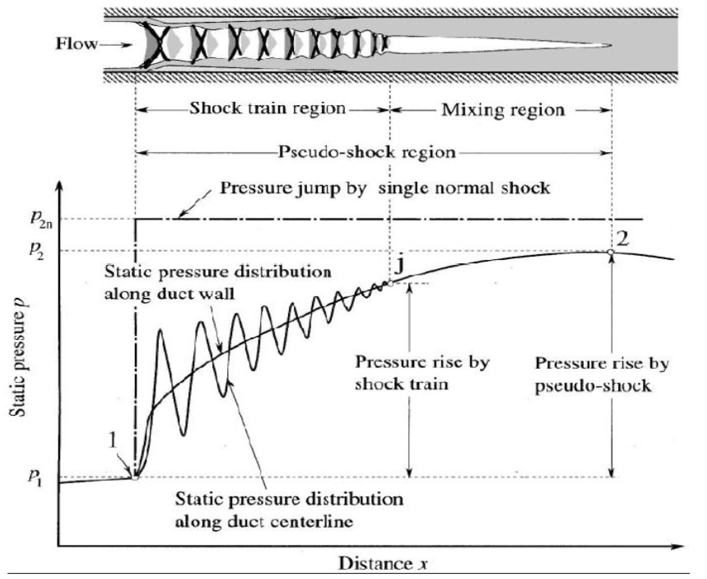
Figure 2.
Computational Domain and Initial Conditions for Sod’s Shock Tube.
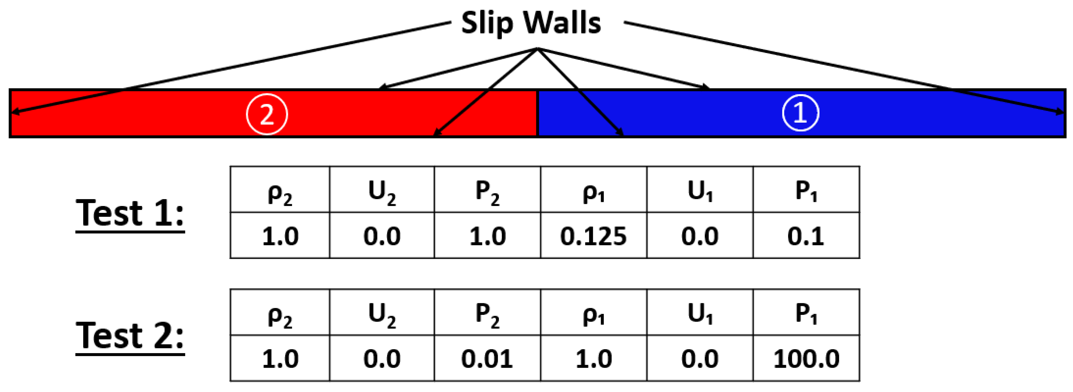
Figure 3.
Code Verification: Comparison of Numerical Results with Exact Solution at t = 0.25 s.
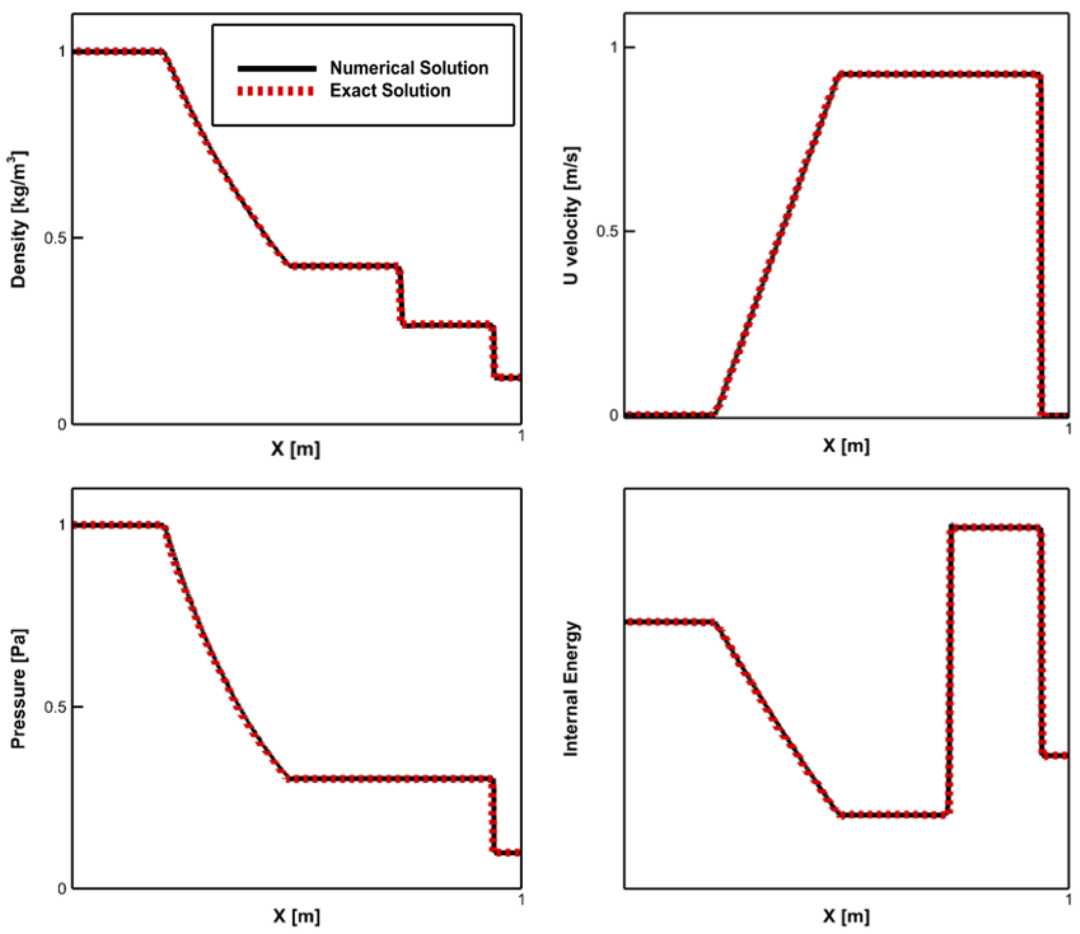
Figure 4.
Code Verification: Comparison of Numerical Results with Exact Solution at t = 0.035 s.
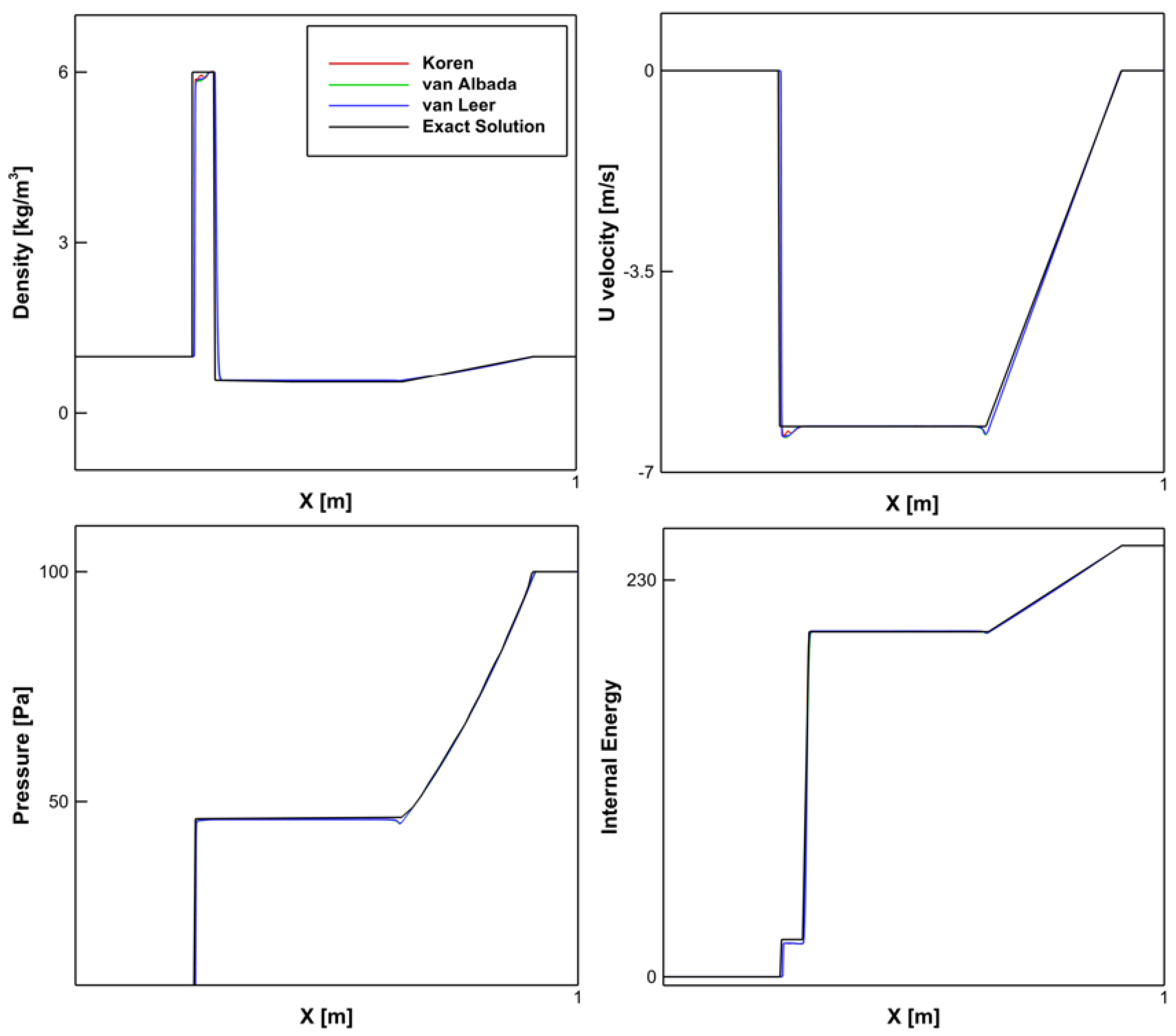
Figure 5.
Computational Domain: Schematic of Quarter Section of the Back-pressured Isolator with Boundary Conditions.
Figure 5.
Computational Domain: Schematic of Quarter Section of the Back-pressured Isolator with Boundary Conditions.
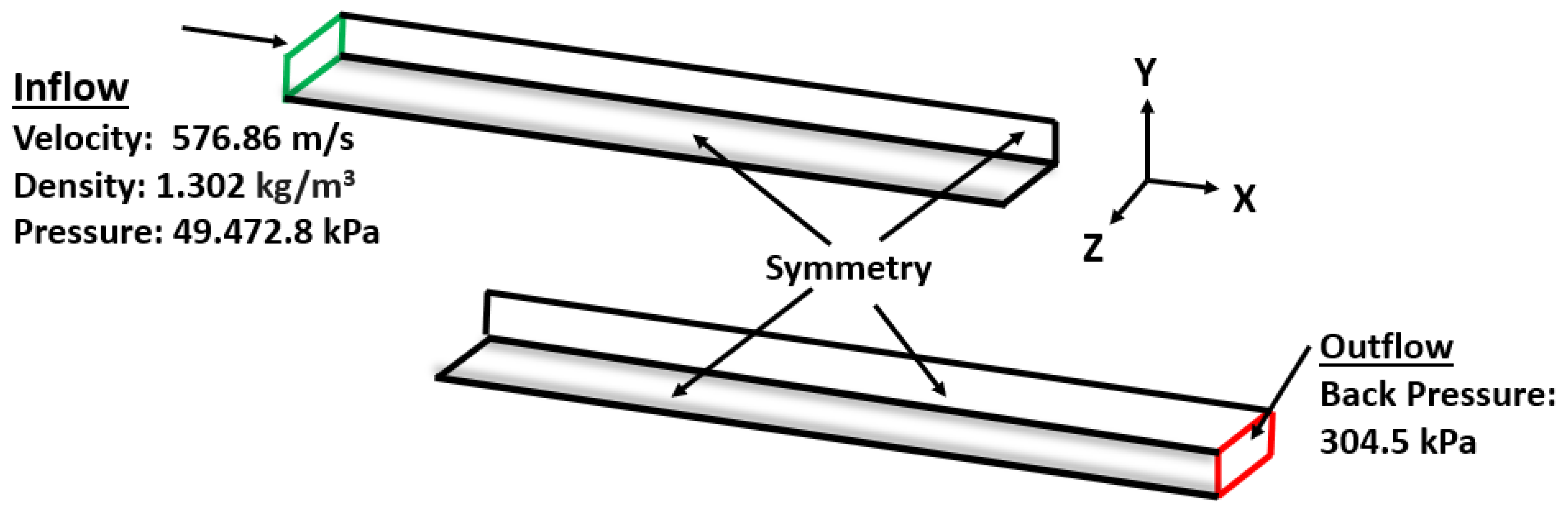
Figure 6.
Model Validation with IDRL Isolator - Static Pressure on Side Wall centerline (left) and Top Wall centerline (right).
Figure 6.
Model Validation with IDRL Isolator - Static Pressure on Side Wall centerline (left) and Top Wall centerline (right).
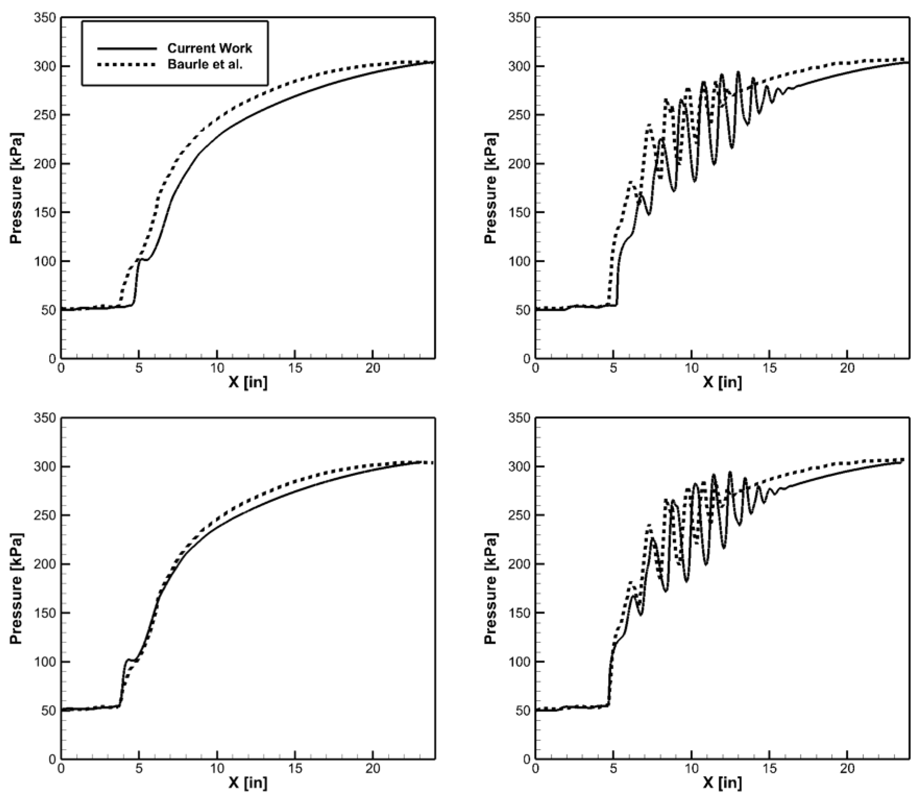
Figure 7.
Isolator Contours: (a) Static Pressure, (b) Eddy Viscosity Ratio, (c) Divergence of Velocity, (d) Axial Velocity.
Figure 7.
Isolator Contours: (a) Static Pressure, (b) Eddy Viscosity Ratio, (c) Divergence of Velocity, (d) Axial Velocity.
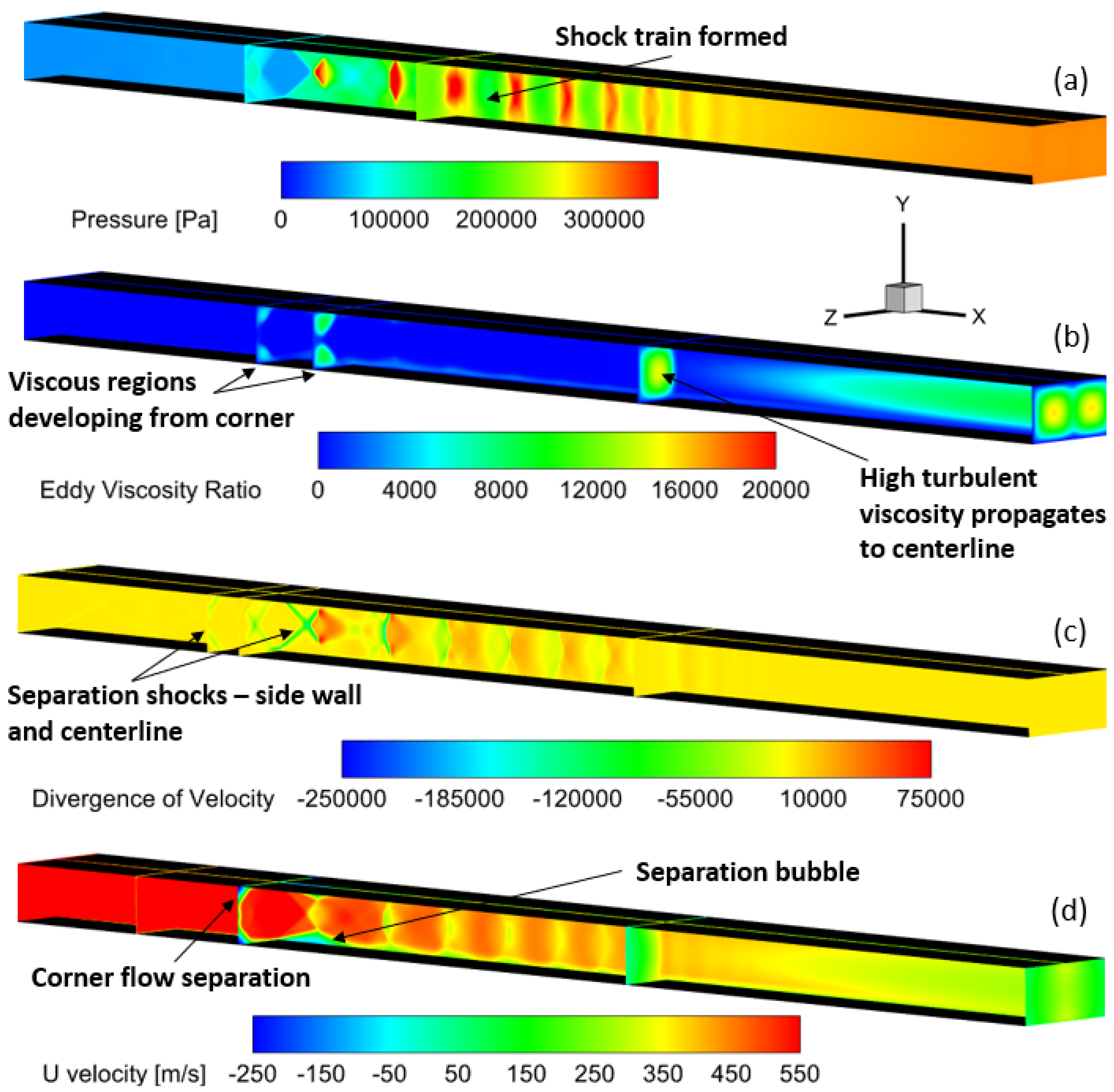
Figure 8.
Isolator Contours with Isothermal Walls: (a) Static Pressure, (b) Eddy Viscosity Ratio, (c) Divergence of Velocity, (d) U Velocity.
Figure 8.
Isolator Contours with Isothermal Walls: (a) Static Pressure, (b) Eddy Viscosity Ratio, (c) Divergence of Velocity, (d) U Velocity.
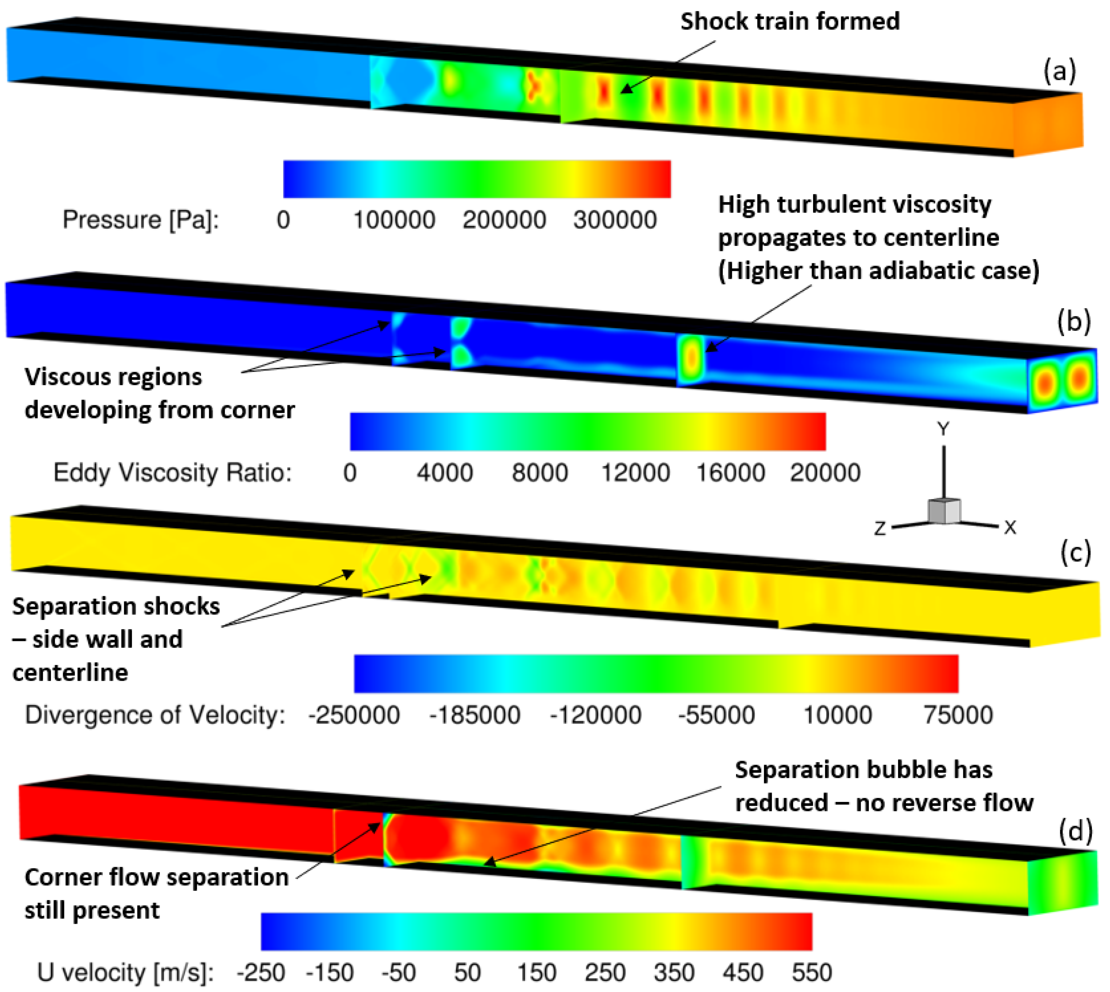
Figure 9.
Effect of Cooled Walls on Static Temperature.
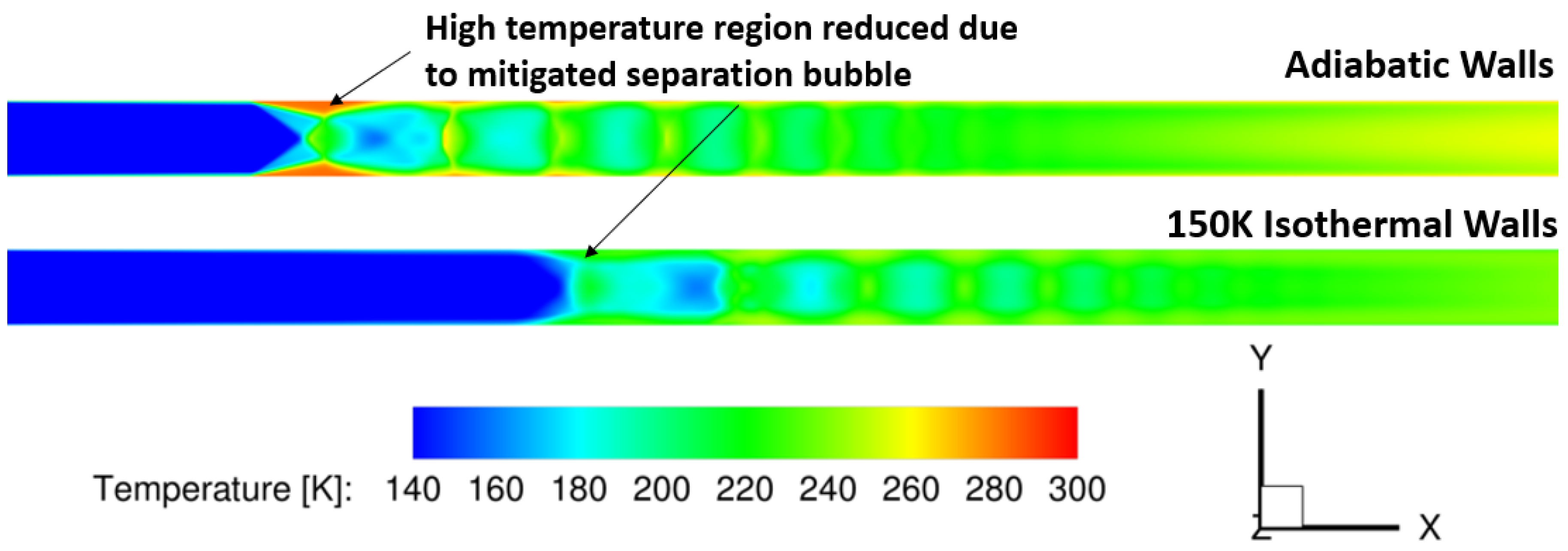
Figure 10.
Effect of Wall Cooling on Divergence of Velocity.
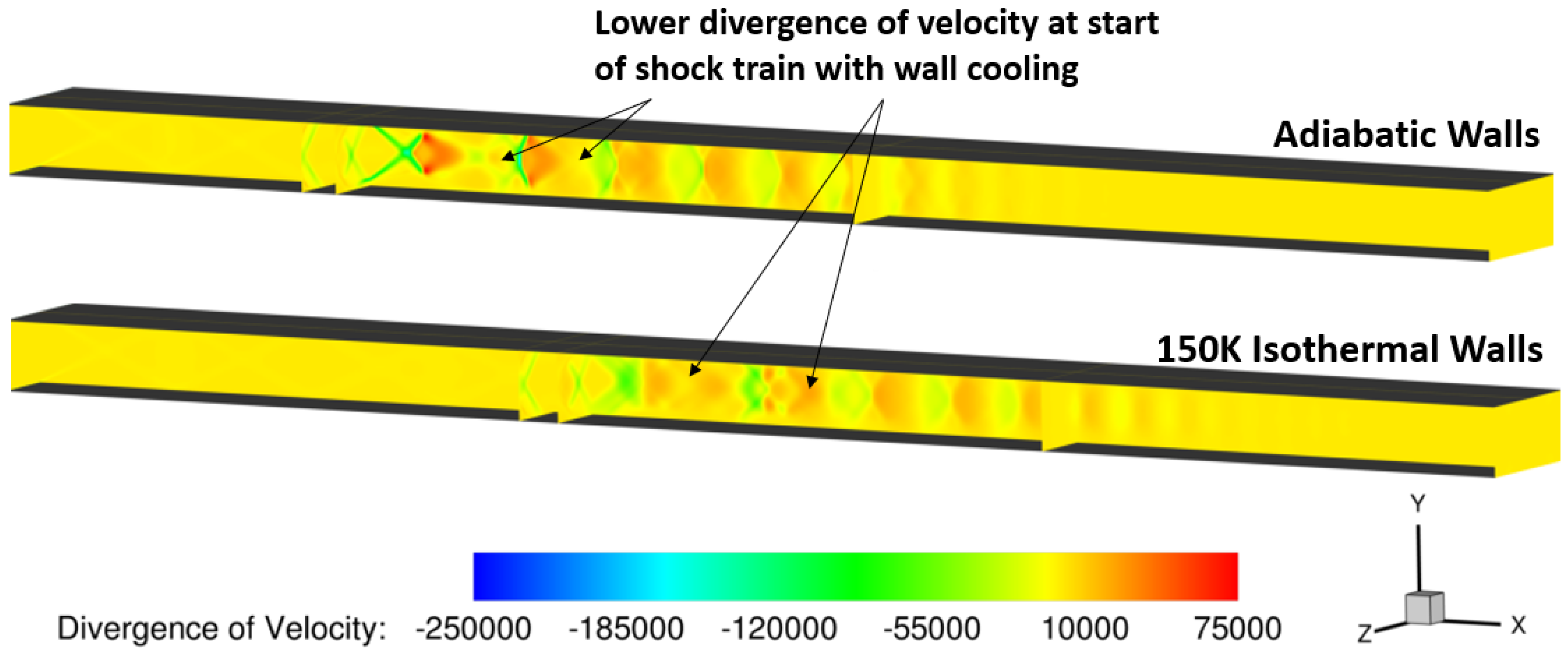
Figure 11.
Effect of Wall Cooling on Mass Flux at Isolator Exit.
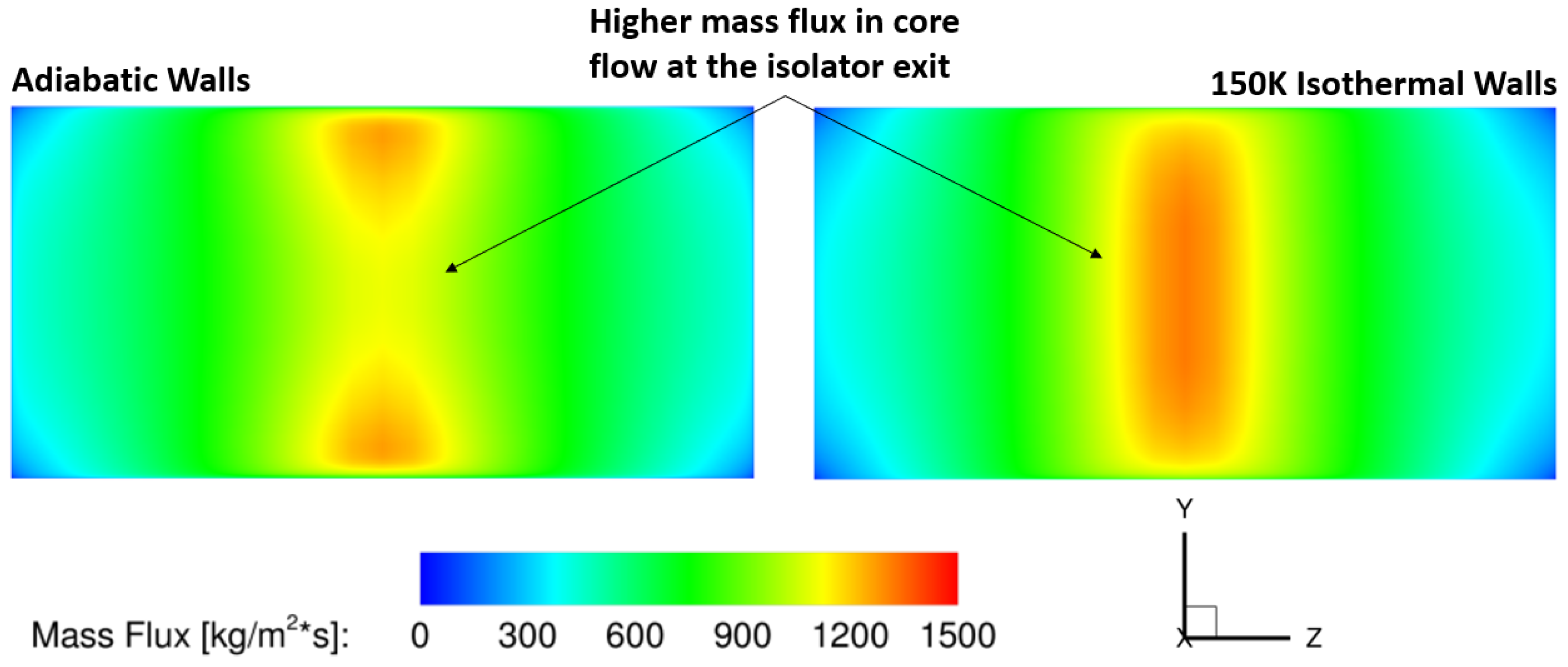
Figure 12.
Effect of Isothermal Cooled Walls on Static Temperature at Isolator Exit.
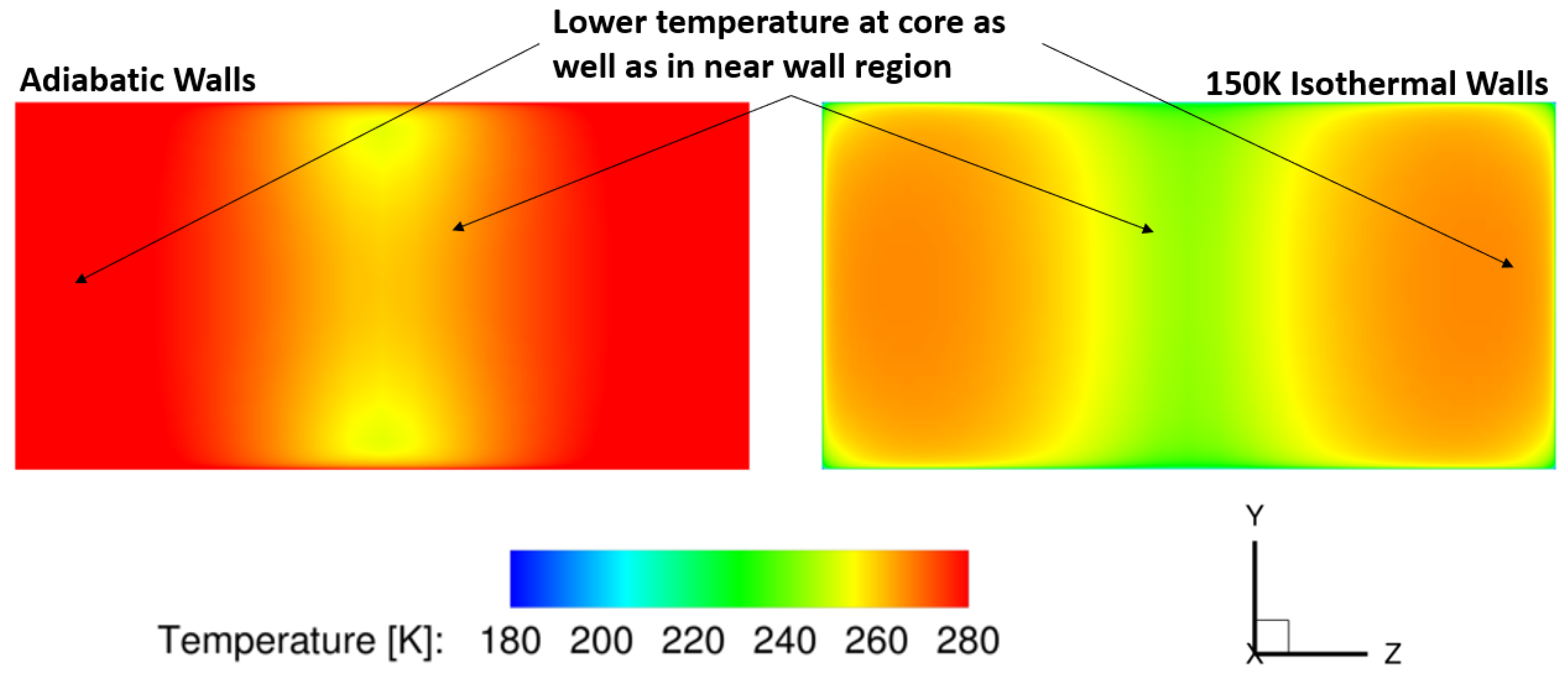
Figure 13.
Effect of Isothermal Cooled Walls Side (left) and Top (right) Centerline Wall Pressure.
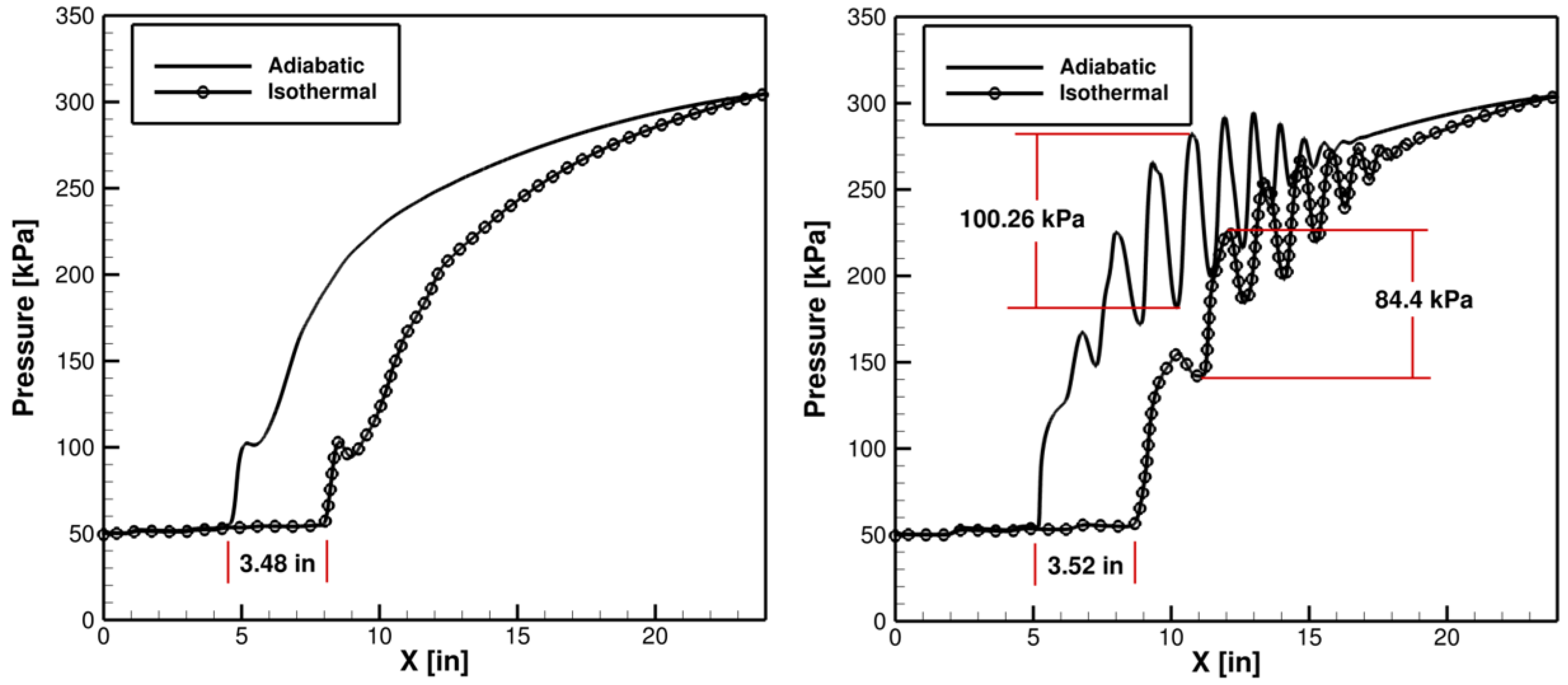
Figure 14.
Computational Domain: Modified Shock Tube with a Velocity Inlet and Pressure Outlet.
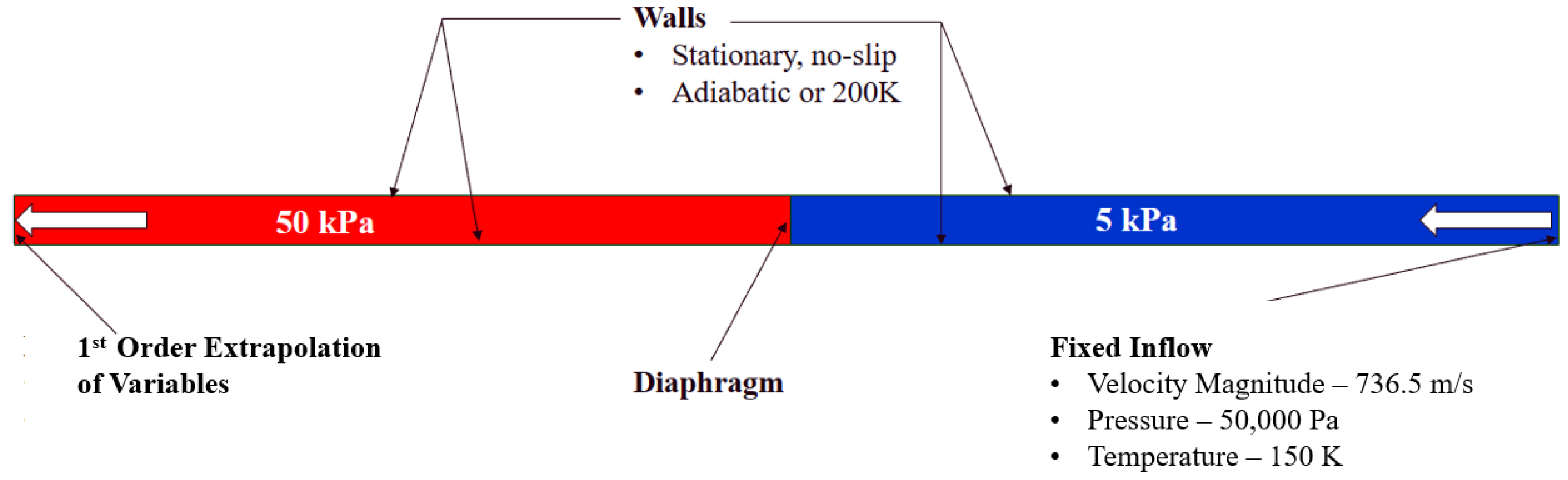
Figure 15.
Static Temperature Contours at Symmetry Plane: Adiabatic Walls with LES.
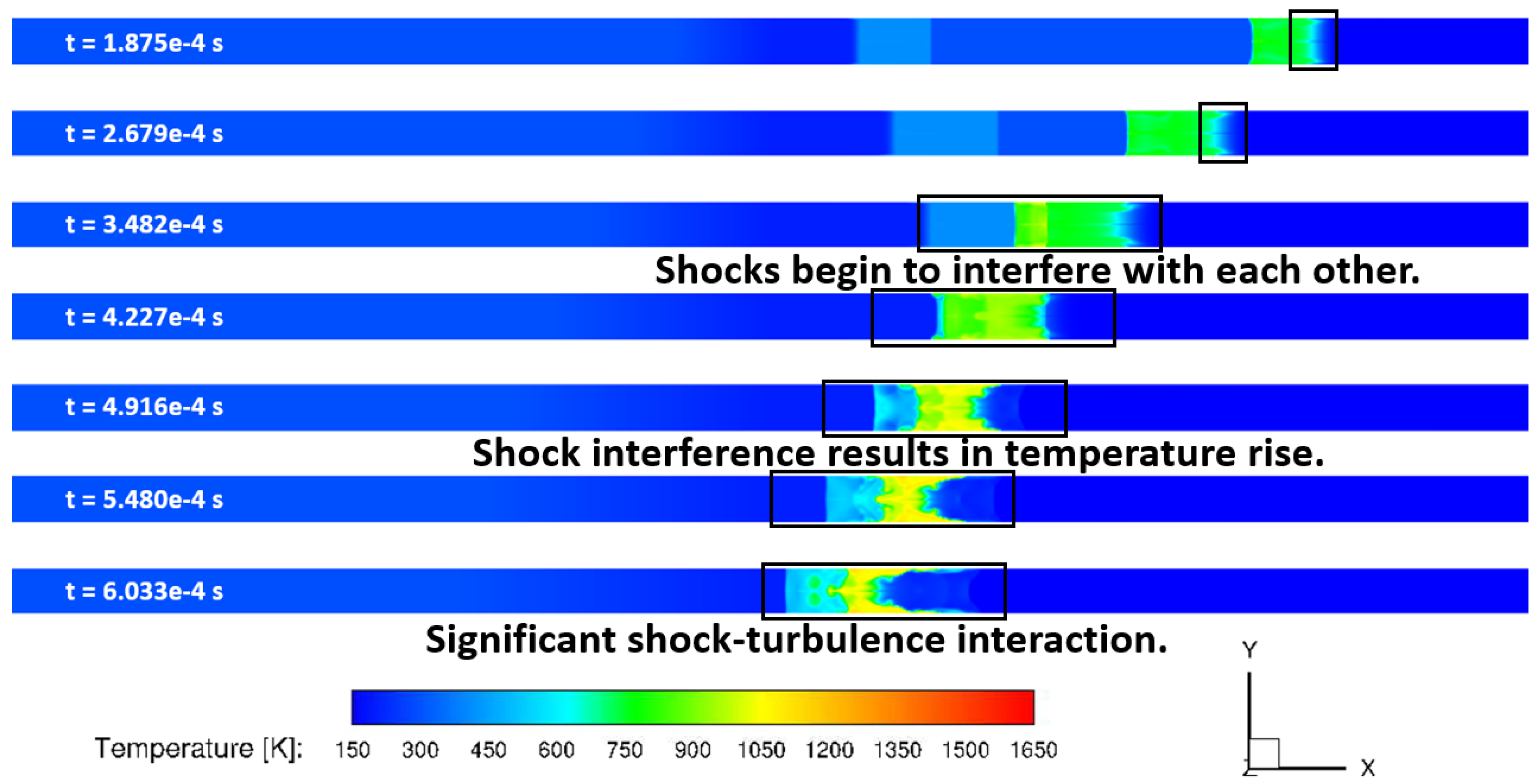
Figure 16.
Static Temperature Contours at Symmetry Plane: Adiabatic Walls with URANS-SA.
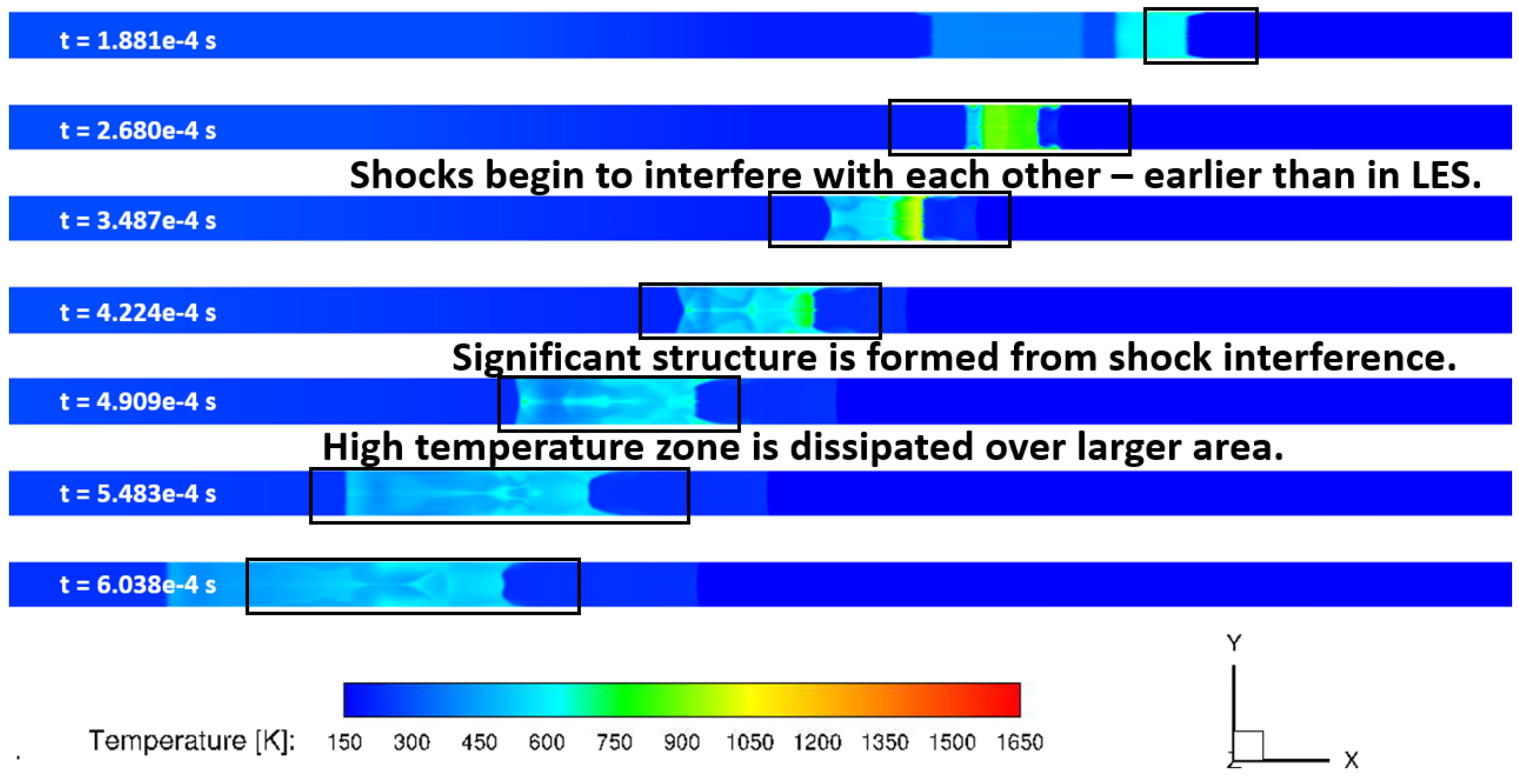
Figure 17.
Density Contours at the Wall: Adiabatic Walls with LES.
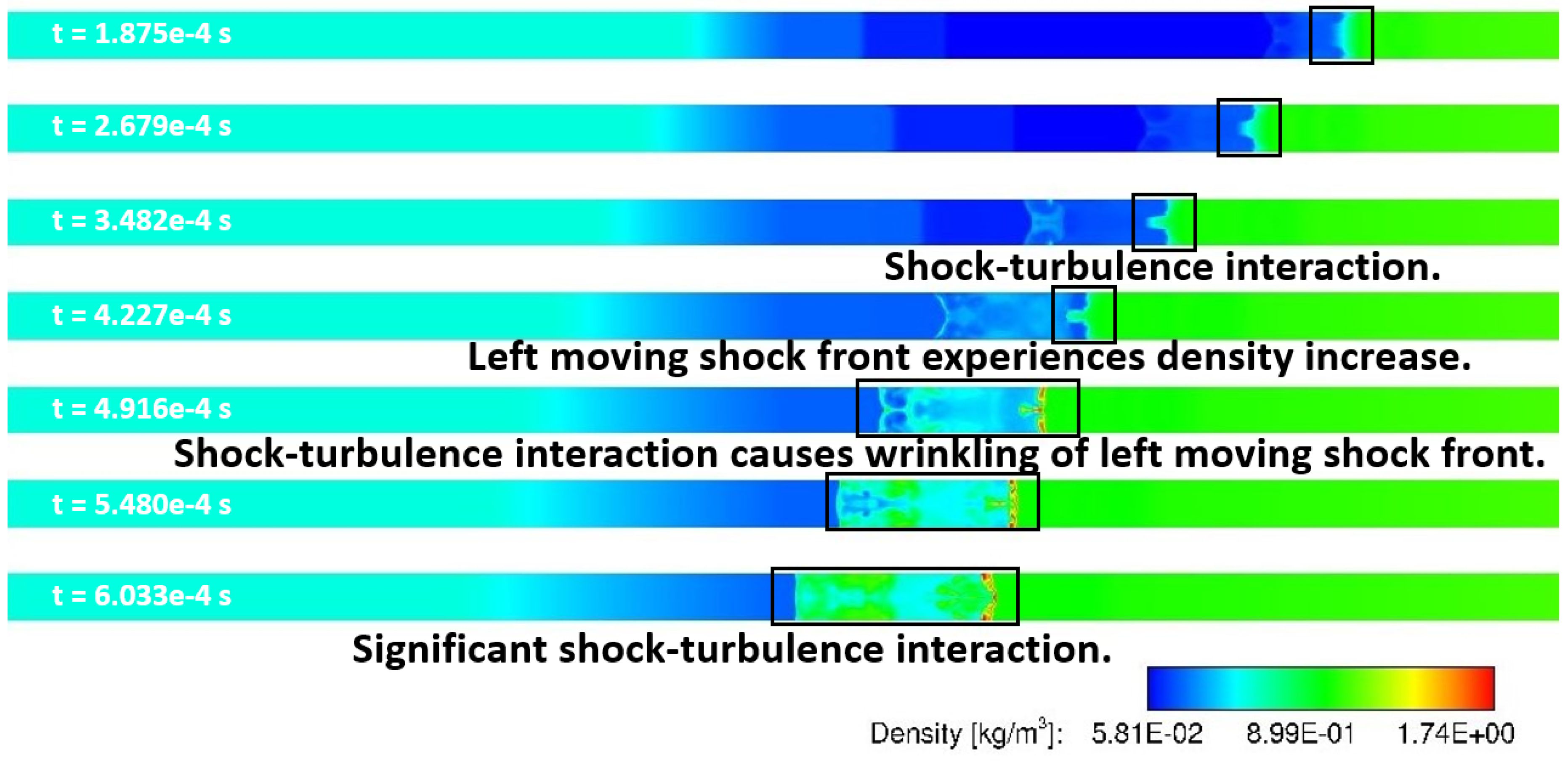
Figure 18.
Density Contours at the Wall: Adiabatic Walls with URANS-SA.
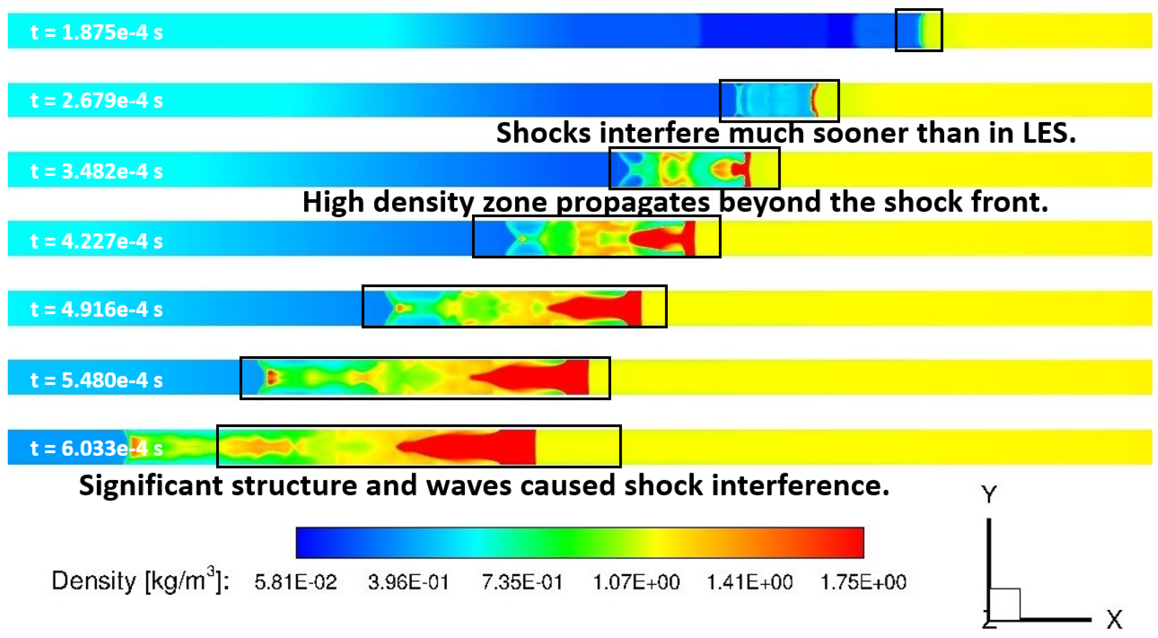
Figure 19.
Static Temperature Contours of Developed Flow: Adiabatic Walls (RANS-SA vs. LES).
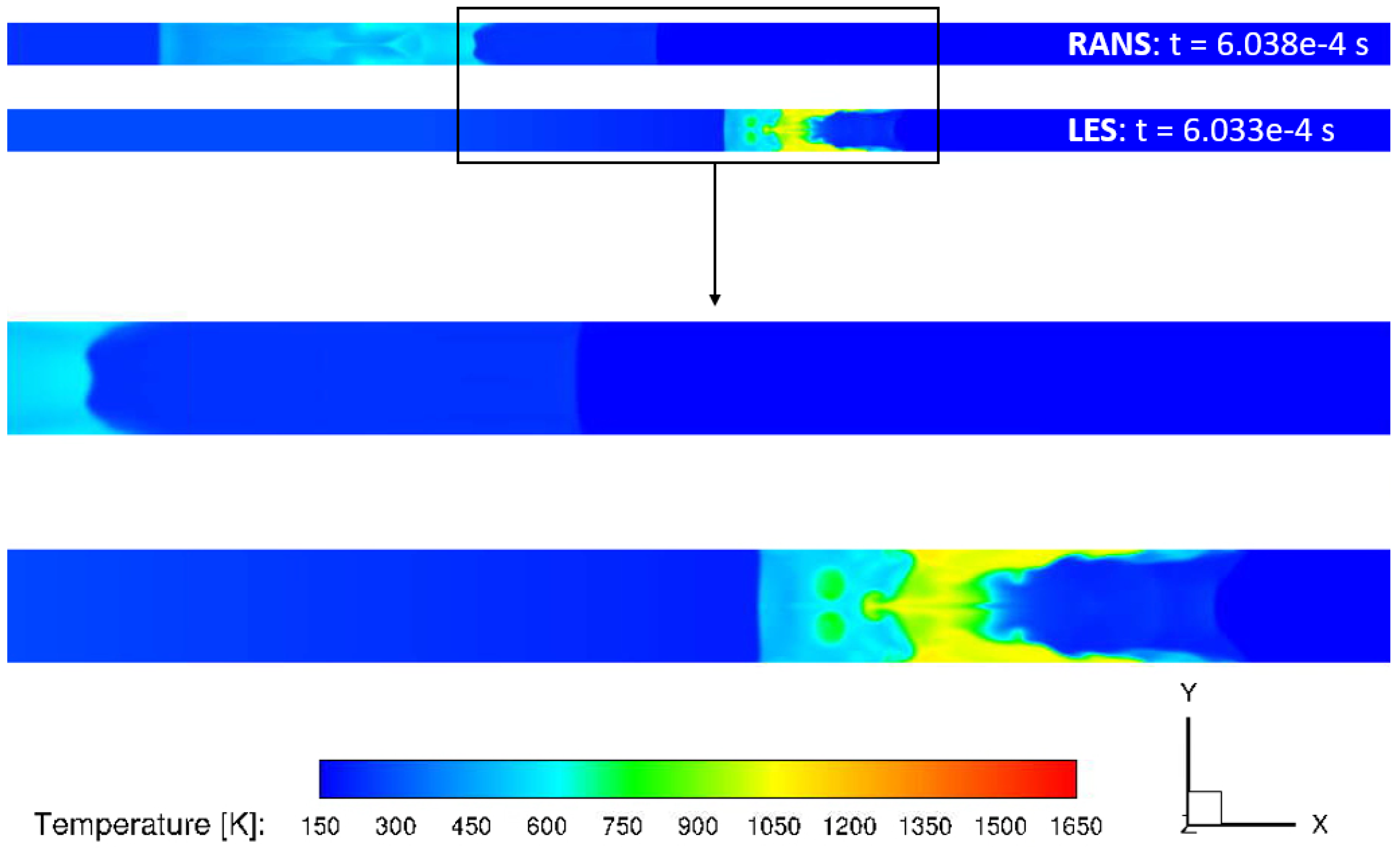
Figure 20.
LES Shadowgraph: Adiabatic Walls.
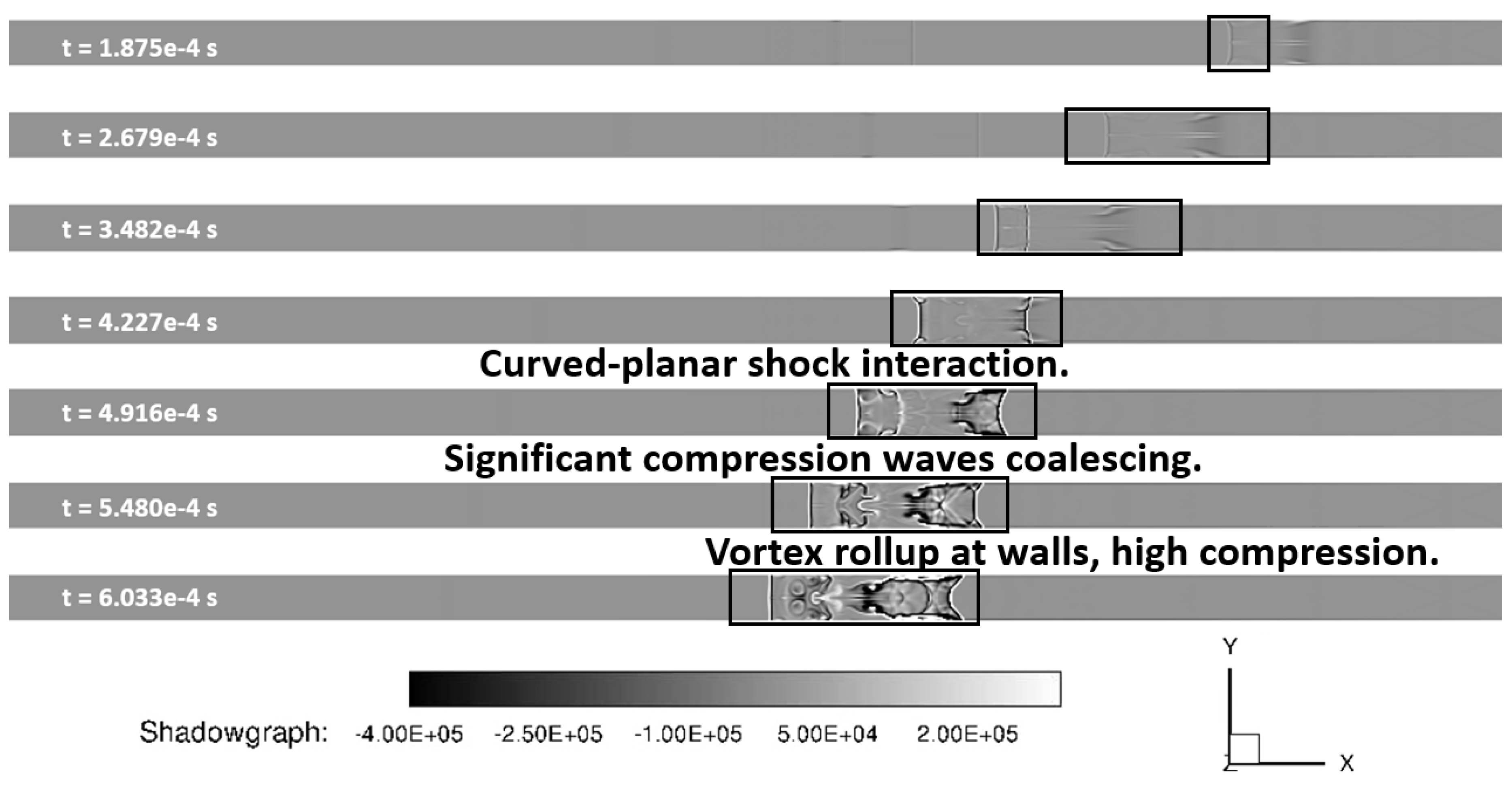
Figure 21.
RANS Shadowgraph: Adiabatic Walls.
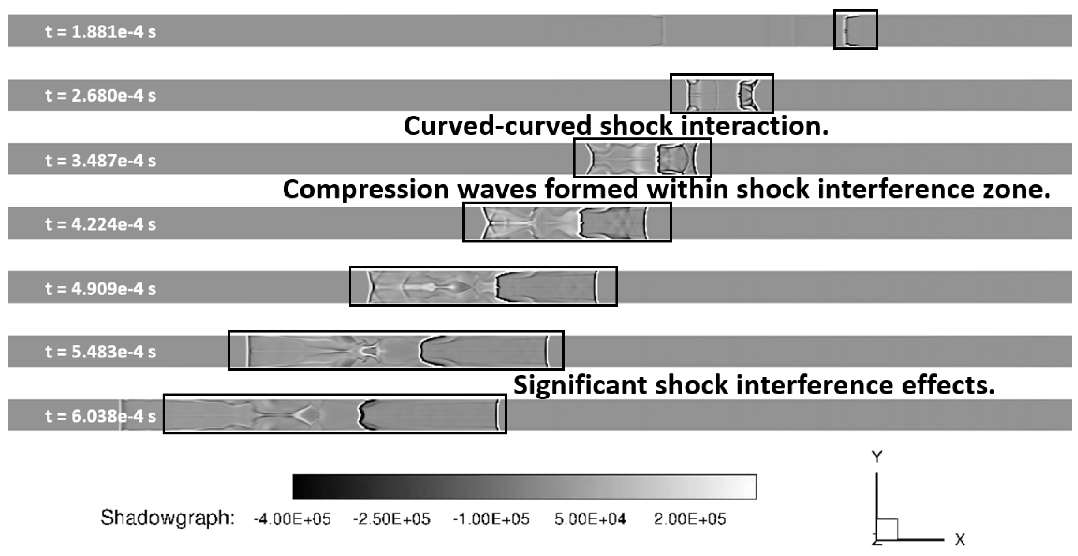
Figure 22.
Mach Number Contours at Symmetry Plane: Adiabatic Walls with LES.
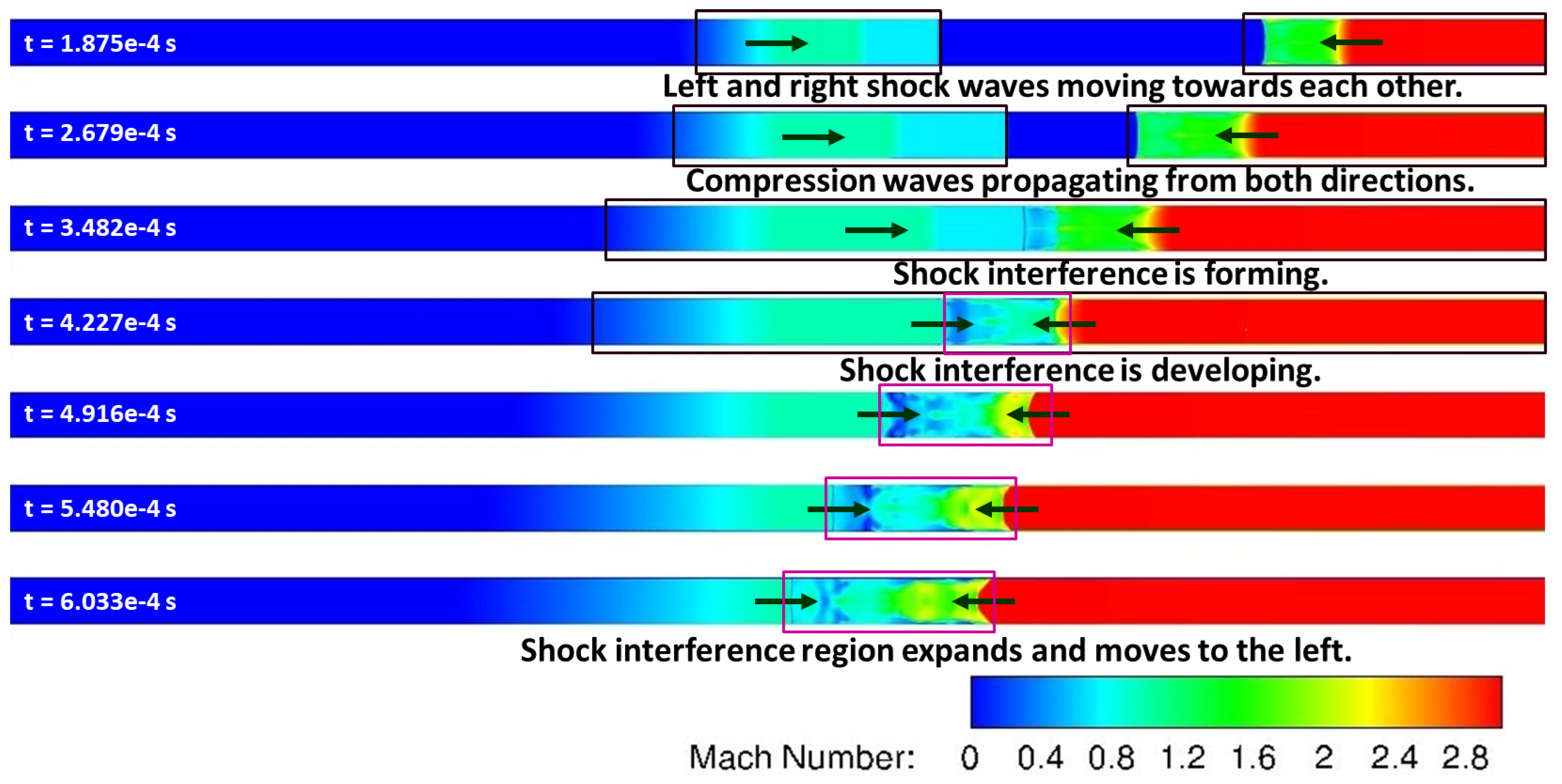
Figure 23.
Pressure Contours at Symmetry Plane: Adiabatic Walls with LES.
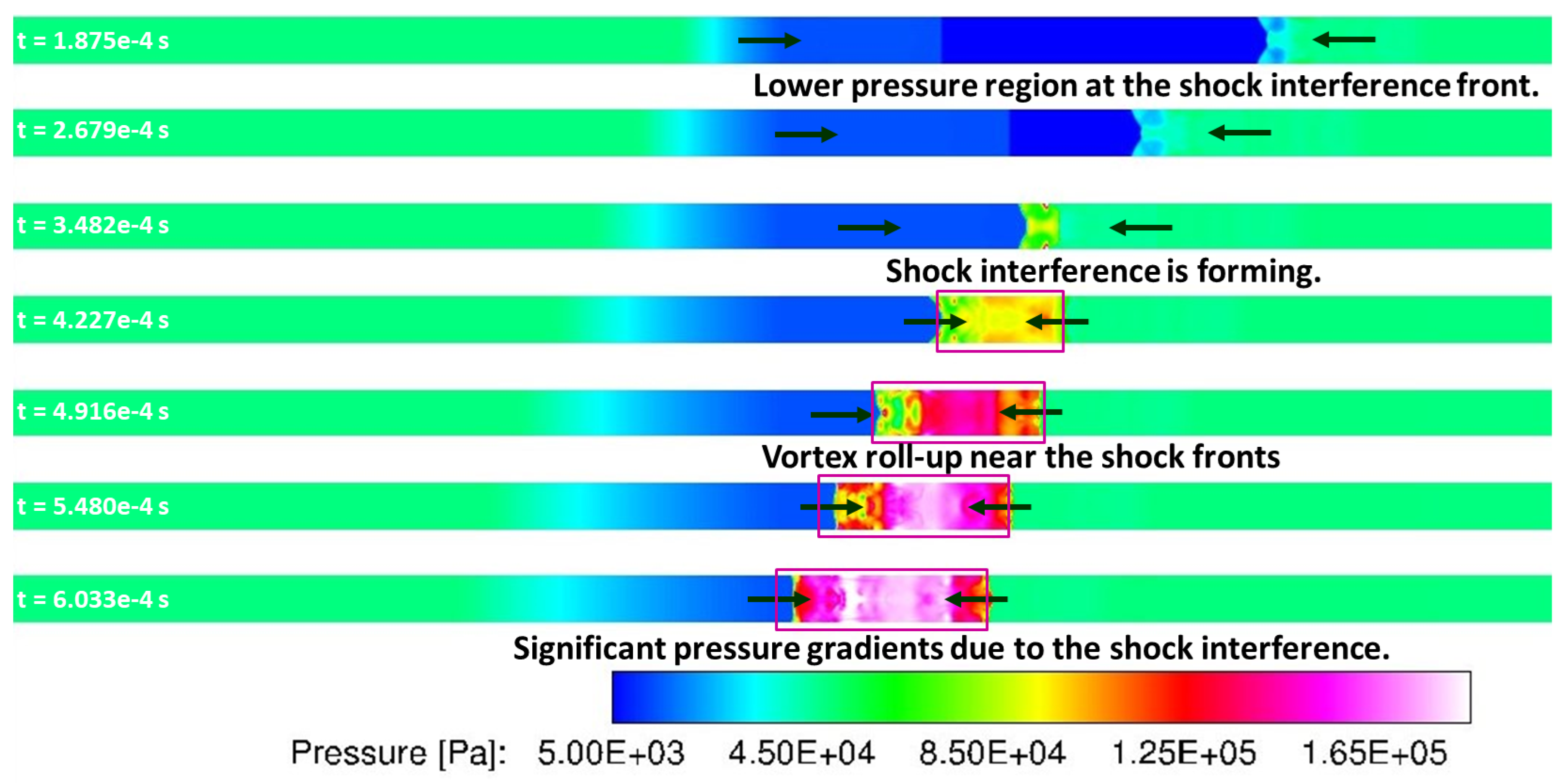
Figure 24.
Eddy Viscosity Ratio Contours at the Wall: Adiabatic Walls with LES.
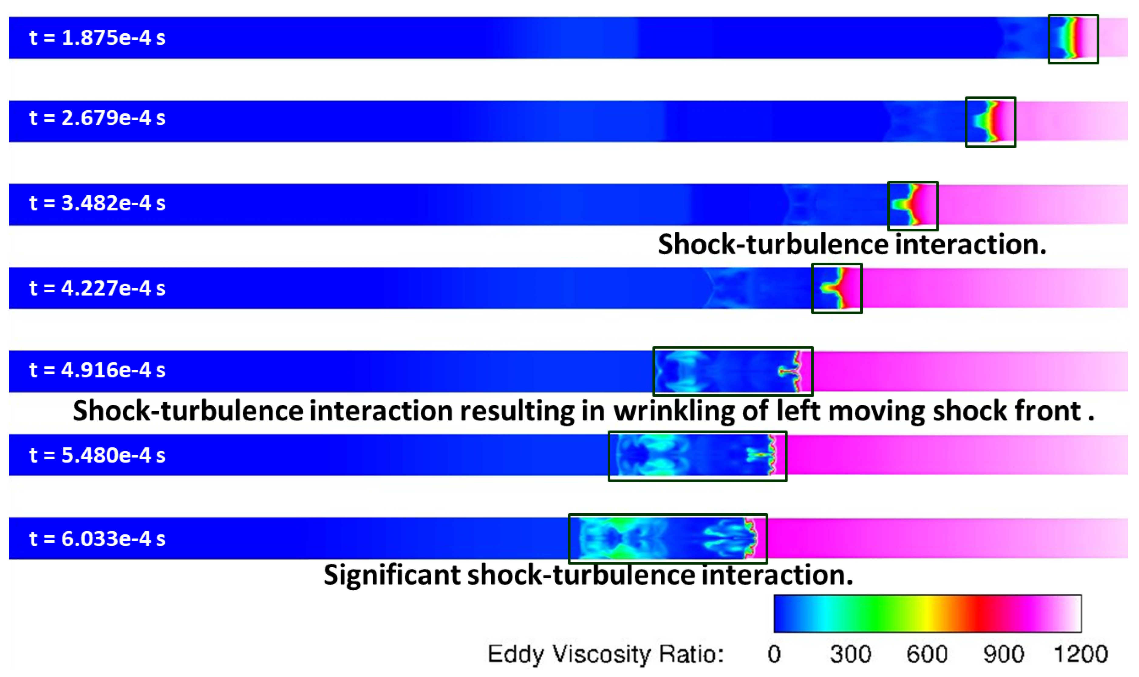
Figure 25.
Wall pressure contours with adiabatic (top) and isothermal (bottom) walls calculated with LES.
Figure 25.
Wall pressure contours with adiabatic (top) and isothermal (bottom) walls calculated with LES.
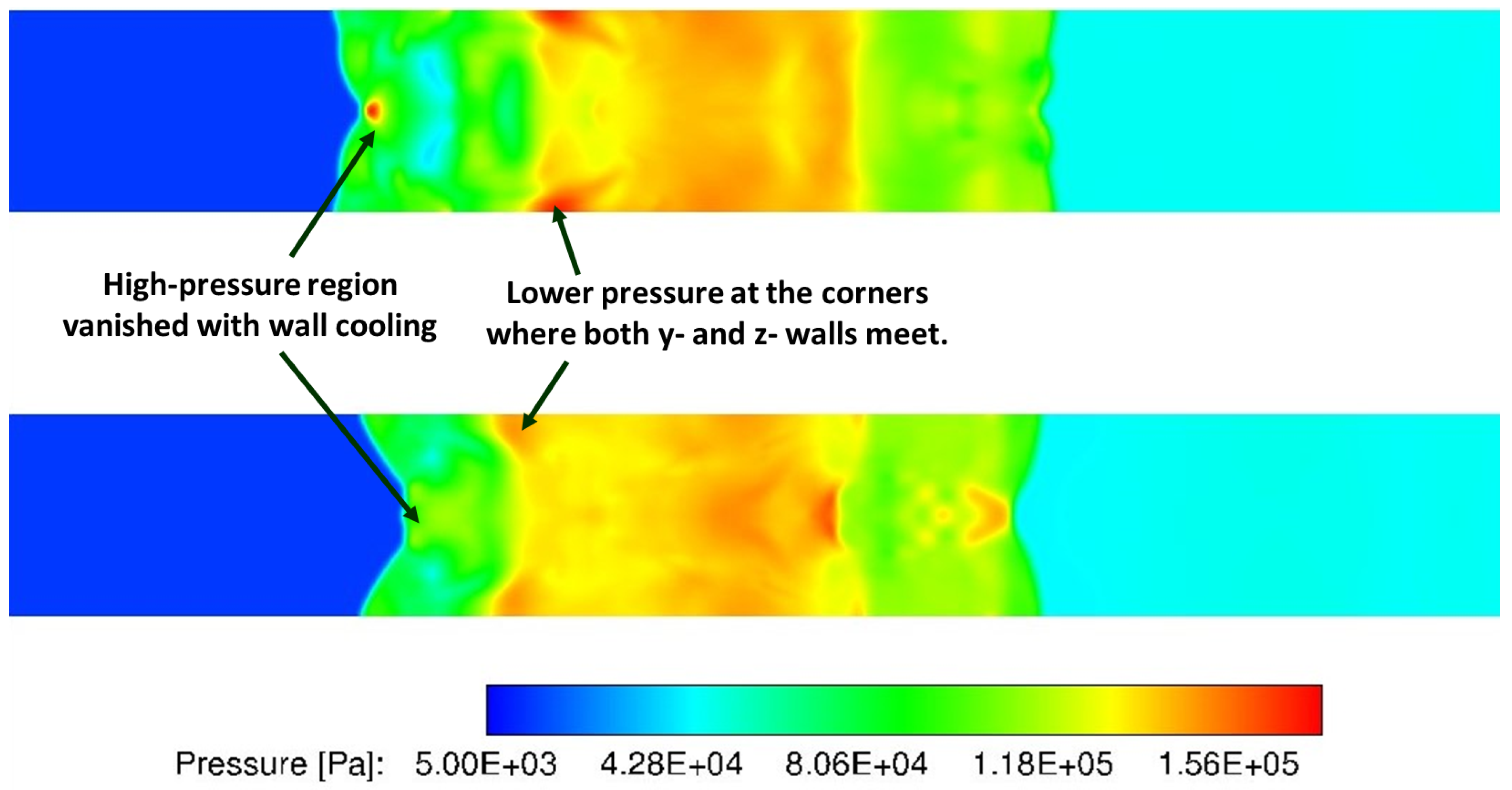
Figure 26.
Static Temperature and Pressure Distribution at t ≈ 4.228e−4 s.
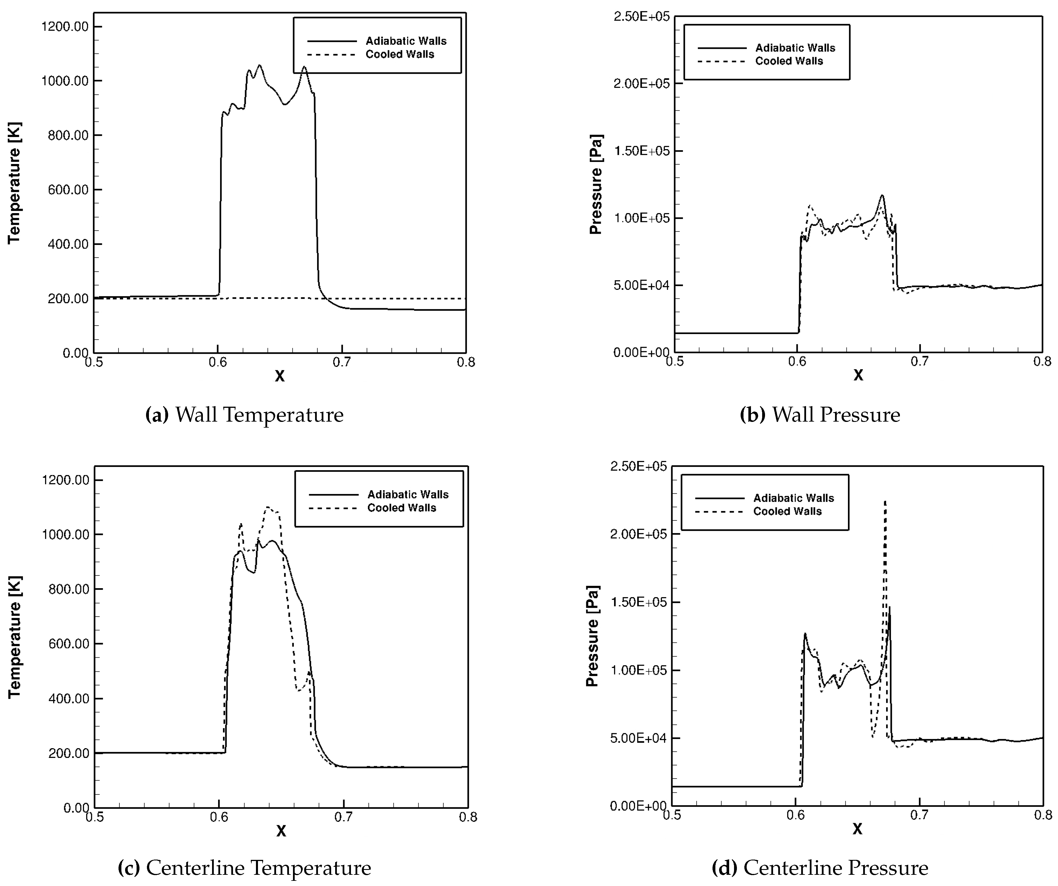
Figure 27.
Static Temperature and Pressure Distribution at t ≈ 4.909e−4 s.
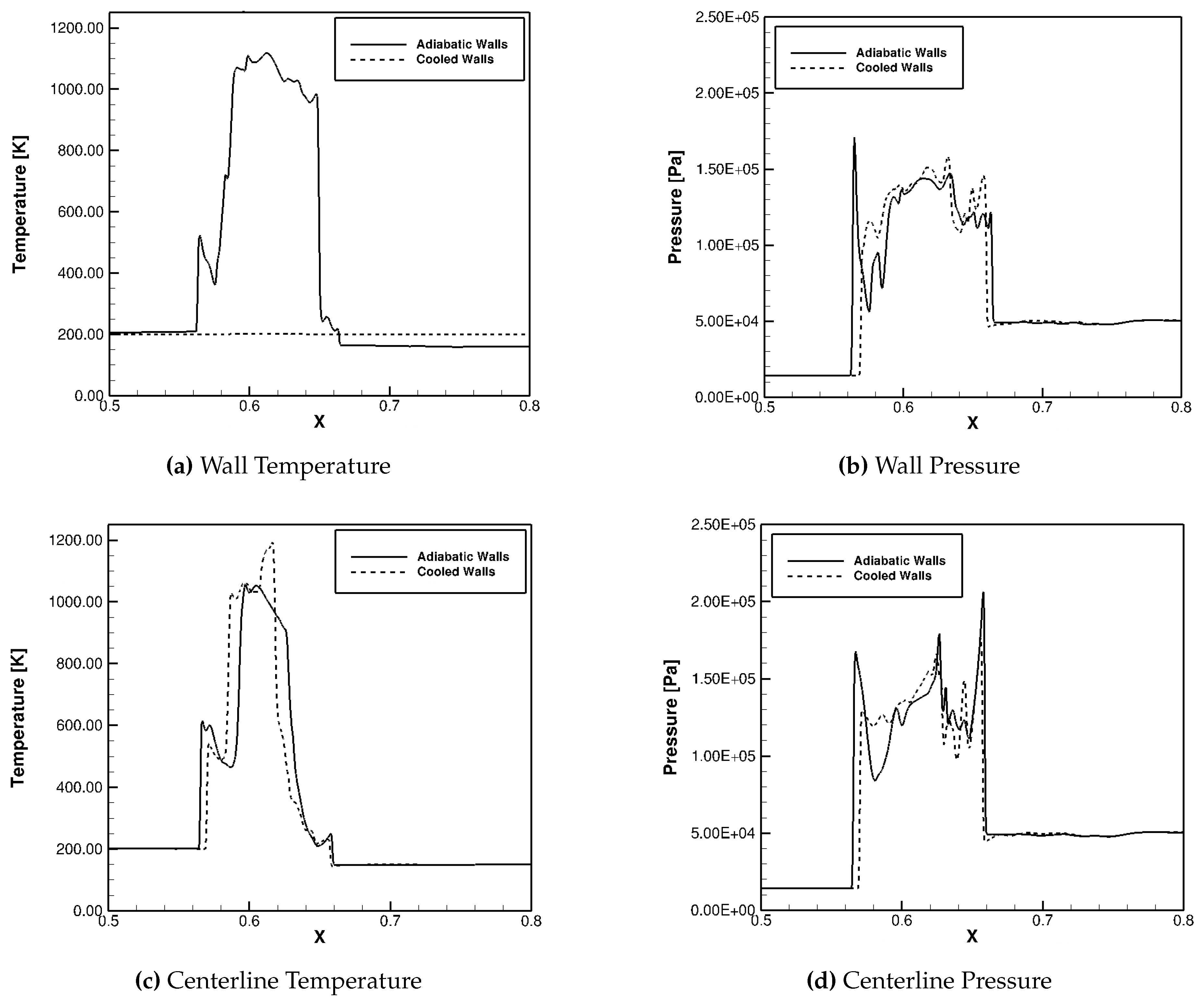
Figure 28.
Displacement Boundary-Layer Thickness with Adiabatic and Cooled Walls.
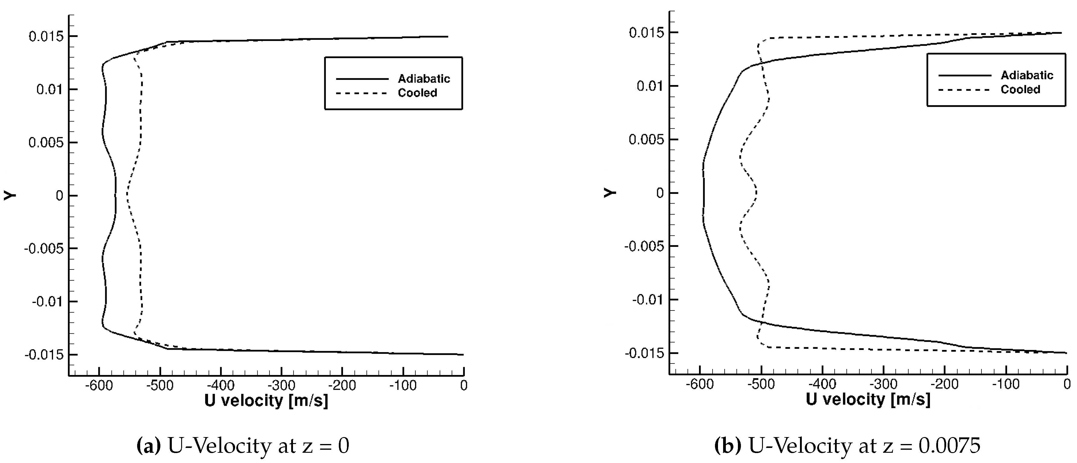
Figure 29.
Static Temperature and Pressure Distribution at t ≈ 4.225e−4 s with 300K Inflow.
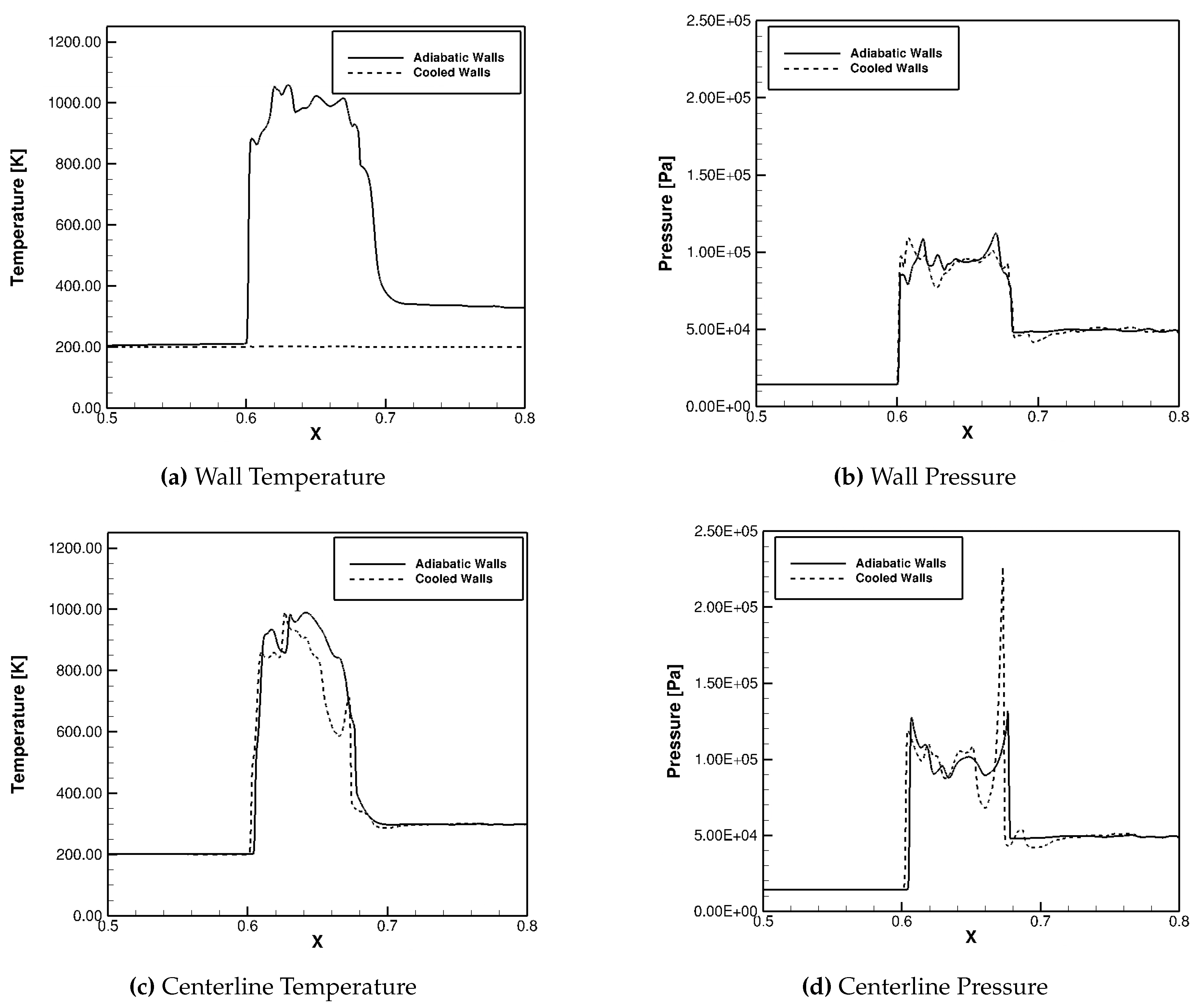
Figure 30.
Static Temperature and Pressure Distribution at t ≈ 4.905e−4 s with 300K Inflow
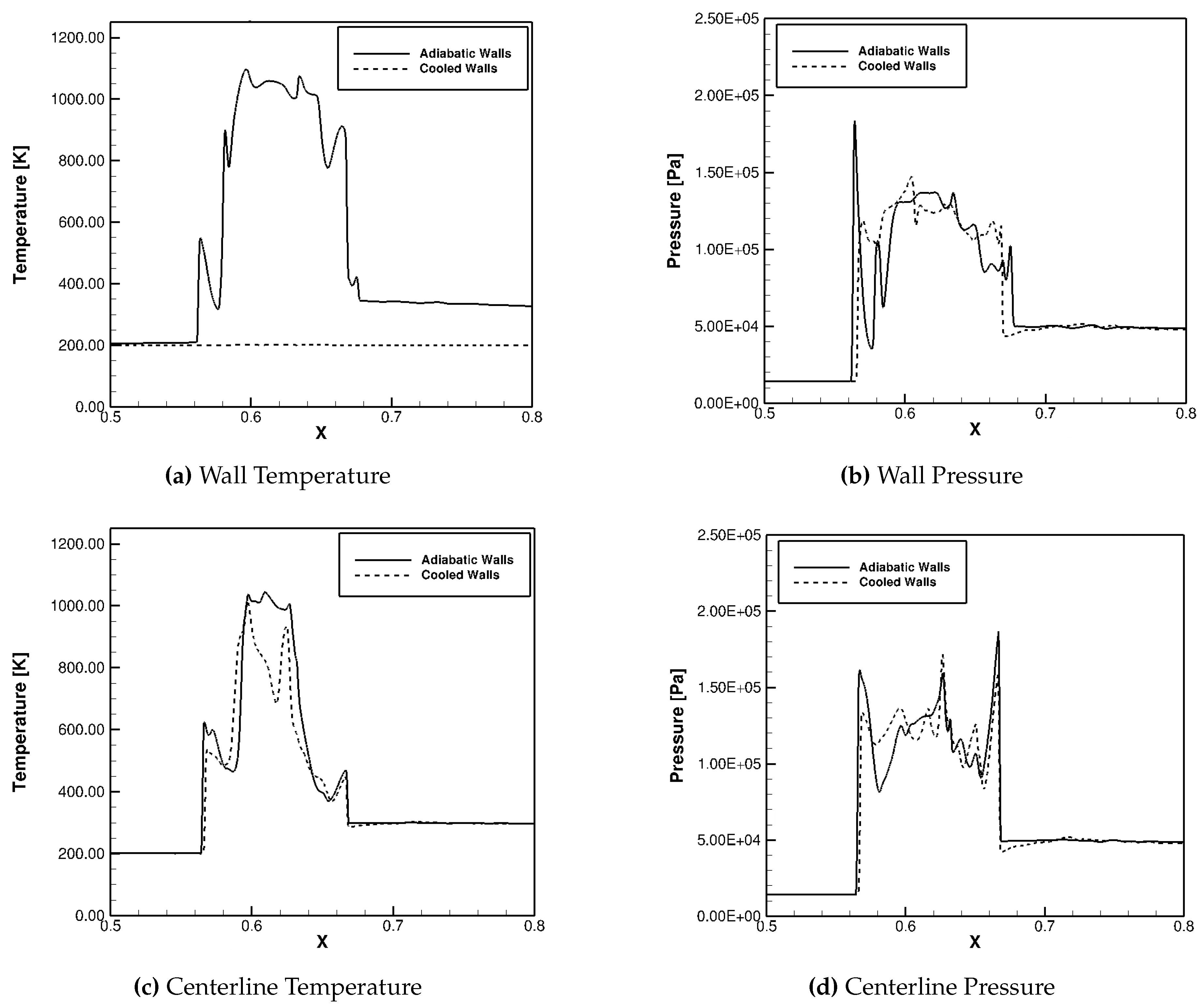

Table 1.
Numerical Methods, Mesh, and Model Specifications Utilized for Model Validation.
| Baurle et al. [15] | Current Work | |
|---|---|---|
| Dimensions | 24x0.5x1 [in] | 0.6096x0.0127x0.0254 [m] |
| Mesh (Isolator) | ||
| Points | 2000x160x208* 1000x80x104 |
1000x80x104 |
| Max. y+ | 1.0 | 1.0 |
| Streamwise spacing in first half of isolator | 0.01 h | 0.02 h |
| Streamwise spacing in second half of isolator | 0.01 h → 0.025 h | 0.02 h → 0.025 h |
| Max. grid spacing in vertical and spanwise directions | 0.01 h | 0.02 h |
| Solution Methodology | ||
| Numerics scheme | Incomplete LU | Incomplete LU |
| CFL number | 100 | 100 |
| Flux scheme | LDFSS | LDFSS |
| Flow variable reconstruction scheme | MUSCL, k= | MUSCL, k= |
| Flux limiter | Koren | Koren |
| Model Specifications | ||
| Turbulence Model | Wilcox 1998 | Wilcox 1998 |
| Molecular and Turbulent Pr | 0.72, 0.9 | 0.72, 0.9 |
| Viscosity model | McBride | Sutherland’s Law |
Table 2.
Flow Variables.
| Baurle et al. [15] | Current Work | |
|---|---|---|
| Total Temperature at Entry [K] | 292.91 | 297.90 |
| Nozzle Plenum Pressure or Isentropic Total Pressure [kPa] | 845.29 | 845.29 |
| Isolator Entry Pressure [kPa] | 49.47 | 49.47 |
| Isolator Back Pressure [kPa] | 304.51 | 304.51 |
| Pressure Ratio | 0.360 | 0.360 |
Table 3.
Quantitative Comparison between Measured and Computational Results.
| Baurle et al. [15] | Current Work | ||
|---|---|---|---|
| Shock Foot Location | Top Wall Centerline | 4.69 inches | 5.21 inches |
| Side Wall Centerline | 3.74 inches | 4.60 inches | |
| Shock-train Length (top-wall centerline) | 8.62 inches | 11.26 inches | |
Disclaimer/Publisher’s Note: The statements, opinions and data contained in all publications are solely those of the individual author(s) and contributor(s) and not of MDPI and/or the editor(s). MDPI and/or the editor(s) disclaim responsibility for any injury to people or property resulting from any ideas, methods, instructions or products referred to in the content. |
© 2025 by the authors. Licensee MDPI, Basel, Switzerland. This article is an open access article distributed under the terms and conditions of the Creative Commons Attribution (CC BY) license (http://creativecommons.org/licenses/by/4.0/).
Copyright: This open access article is published under a Creative Commons CC BY 4.0 license, which permit the free download, distribution, and reuse, provided that the author and preprint are cited in any reuse.


