
Submitted:
23 May 2025
Posted:
26 May 2025
You are already at the latest version
Abstract
This paper proposes an experimental procedure based on Hyperspectral Imaging (HSI) combined with statistical classification for assessing archaeo‐paleoanthropological stratigraphic deposits at the Gran Dolina site (TD10 unit), located in the Sierra de Atapuerca (Burgos, Spain). Representative spectral reflectance signatures were determined and analyzed using HSI measurements and statistical classification methods in natural light conditions across various capture distances. This study aims to characterize and quantify cave sediments by defining spectral models for feature classification and spectral similarity analysis, evaluating the strengths and limitations of spectral captures at this specific site. HSI technology enhances the analysis and identification of materials at an internationally recognized reference site for Human Evolution studies. The hyperspectral imaging assessment of archaeo‐paleoanthropological stratigraphic deposits emerges as an innovative digital tool, revolutionizing the sustainable management of Cultural Heritage and Environmental Sciences by enabling advanced material identification and stratigraphic analysis.
Keywords:
hyperspectral imaging
; statistical classification
; cultural heritage
; endmember extraction
; Spectral Angle Mapper
; stratigraphy
; Paleolithic site
1. Introduction
Spectroscopy has long served as a valuable quantitative tool in laboratory analysis, with various research methods evolving over time [1]. Recently, multiple scientific disciplines have adopted image spectroscopy, which is widely used as both a qualitative and quantitative research tool in mineralogy, agriculture, and environmental resource management. The Hyperspectral Imaging (HSI) system, especially in the Visible Infrared (VIR) and Near Infrared (NIR) ranges, provides extensive electromagnetic spectral data, capturing optical information of investigated samples. By combining high-spectral-range imaging with artificial intelligence analysis, HSI constitutes a non-destructive quality assessment method, enabling the analysis and identification of the spectral-spatial variation in materials or objects [2].
HSI data is derived from airborne, satellite, or near-field sensors. Airborne Imaging Spectroscopy (AIS) has applications in diverse fields such as soil erosion monitoring [3], riverbed morphodynamics [4], and rapid mapping of areas affected by natural disasters [5]. AIS also supports agronomic research, aiding in crop management and variability analysis [6], as well as landscape condition assessments, including changes in vegetation distribution due to climate change and land use shifts, a growing focus in landscape conservation worldwide [7,8,9].
In Cultural Heritage studies, multispectral and HSI techniques have proven effective for material classification [10,11]. MSI has facilitated the study of archaic cultures, where vegetation cover, soil composition, or depth-specific archaeological features pose significant challenges [12]. However, only recent studies have focused on detailed spectral analysis in geoarchaeology [13,14,15]. Hyperspectral imaging applied to sediment cores remains a developing tool, with potential to enhance the understanding of paleo-environmental processes [13]. NIR spectroscopy, for instance, has been useful in stratigraphy studies, complementing wet chemical analyses in archaeological excavations [14]. New methods for analyzing archaeological airborne spectroscopy data, such as red edge inflexion point (REIP) and distribution fittings, further maximize remote-sensing data utilization [15].
While constraints still limit hyperspectral remote sensing in geological applications, prior AIS-based studies have shown promising results using processing techniques like Principal Component Analysis and Vegetation Indices [16]. This technology has the potential to reveal environmental and geological features critical to the mining and environmental geology industries, with one of its significant applications being the production of geological maps that classify surface materials, including minerals and rocks.
The excavation of archaeological sites is key to understanding and disseminating the heritage of past societies, particularly in Paleolithic sites, where human activity left few structural imprints. In these contexts, precise identification and spatial documentation of archaeological elements within their stratigraphic context is essential for interpreting site formation processes.
Presently, excavation monitoring encompasses diverse methods, including detailed photographic documentation, topographic techniques (grids, Total Stations, GNSS), and 3D mapping [17,18,20]. However, traditional techniques lack the capacity to analytically differentiate elements based on physical properties. Advances in image spectrometry, including high-capacity sensors, have enabled new areas of analysis and research [12,13,14,16]. This study applies HSI technology to identify and characterize the spectral response of stratigraphic contexts in the Paleolithic TD10 unit at the Gran Dolina site (Sierra de Atapuerca, Burgos, Spain), enhancing analytical potential by providing complementary information for the identification, classification, and characterization of materials in an archaeo-paleoanthropological context. Previous research explores an emerging scenario in the use of HSI for material analysis, demonstrating its capability to enhance the identification and preservation of historical artifacts. [21].
1.1. Background and Geoarchaeological Characteristics
In the Sierra de Atapuerca (Burgos), Lower Paleolithic sites are preserved within sedimentary fills contained in a multilevel cave system [17,18], associated with Pleistocene fluvial levels imposed by the Arlanzón River [19,20]. The sediments containing archaeological remains were deposited by gravitational and water flow processes, forming breccias (composed of blocks and mud), gravel, sand, silt, and clay [22,23,24]. These sediments contain human fossils, stone tools (made of chert, quartzite, quartz, sandstone, and limestone), and faunal remains, spanning from the Early to the Middle Pleistocene [26,27,28,29].
This study focuses on the Gran Dolina site, a 25-meter-thick cave infilling within the intermediate endokarst level [30], generated by the phreatic level associated with the Arlanzón fluvial terrace T3 during the Early Pleistocene [31,32]. The Gran Dolina sequence is divided into 12 lithostratigraphic units, numbered from bottom to top (TD1-TD11, with a later-defined TD8-9 unit) [22,23,24,35]. Units TD1 and TD2 are classified as cave interior facies, while TD3 to TD11 are categorized as cave entrance facies [23]. From TD4 to TD11, the cave was progressively filled by sediment inflow from a proximal entrance, continuing until complete silting occurred in the TD11 unit. These entrance facies are the result of sedimentary gravity flow processes—including debris fall, debris flow, and mud flow—as well as fluvial processes such as channel deposits, floodplain sediments, and decantation features [23]. The Gran Dolina site contains significant Early and Middle Pleistocene archaeo-paleontological levels [35,36], with documented lithic tools, as well as faunal and human remains [23,26,28,29,35]. Notably, the TD6 unit contains human remains, lithic tools, and fauna dated to approximately 0.8–0.9 million years ago [26,28], while the TD10 unit, interpreted as a human campsite dating back to about 0.35 million years ago, has yielded two important archaeological assemblages with over 30,000 lithic remains and 99,000 faunal remains [28]. The TD10 unit comprises a sequence of debris flow facies deposited from the main western entrance, with limited side entrances and occasional breakdown events [23,24]. This unit is further subdivided into four sub-units, labeled from bottom to top as TD10.4 to TD10.1, each containing six described sedimentary facies (Table 1, Figure 1) [23].
The first entry in this unit, TD10.4, comprises mud and gravel layers that have been interpreted as debris flow facies F, along with mudflows, channels, and floodplains [23]. The channel facies, located centrally within the section, consist of approximately 70% centimeter-sized gravel and 30% mud. Mudflow and floodplain facies occupy the lateral parts of the section, mainly composed of mud with some gravel inclusions. Clasts potentially dislodged from the cave roof are noted near the walls. Visual color assessments, performed according to the Munsell soil color charts, reveal that these facies exhibit a yellowish-red 5YR 5/8 hue, although some layers display a slightly more yellowish tint (Table 2). Additionally, phosphate crusts are present in certain layers of TD10.4, suggesting that the weathering process may be associated with the bat guano deposit found in TD9 [23]. Successive debris flow inputs from the primary western entry, with additional smaller secondary entries, formed sub-units TD10.3, TD10.2, and TD10.1. TD10.3, measuring approximately 80 cm in thickness, contains at least two instances of debris flow facies F (Table 2, Figure 1 and Figure 2). These are grain-supported clasts within a reddish-yellow 5YR 6/8 mud matrix, averaging 15 cm in diameter, with some clasts reaching 35 cm. Near-meter-diameter clasts observed within these layers suggest rockfalls from the cave roof, which may have enlarged existing entries or created new ones, as indicated by debris flow facies F from SE inputs [23]. TD10.2 is a sub-unit approximately 1 m thick, comprising debris flow facies C, D, and F, interspersed with minor layers of channel and decantation facies (Table 2, Figure 1 and Figure 2). The color ranges from strong brown 7.5YR 5/6 in layers with less gravel content to reddish yellow 5YR 6/8 in layers containing more gravel. This sub-unit also exhibits notable lateral facies variation. Channel and decantation facies, about 15 cm thick, are limited to the eastern section where the debris flow facies decrease in thickness, while debris flow facies predominate elsewhere. In TD10.1, the influence of fluvial processes increases, as indicated by thin decantation and channel facies layers found in the central section. However, debris flow facies D and F remain the primary facies in this approximately 1 m thick sub-unit, which represents the final sedimentary layer containing fossil remains at the Gran Dolina site. As with the underlying sub-units, the color varies from reddish-yellow 5YR 6/8 in gravel-rich debris flow facies to yellowish-red 5YR 5/8 in muddier layers. While the color observed in the field and identified via the Munsell soil chart remains relatively uniform, a relationship between the color intensity and the mud content is evident. In general, reddish hues correlate with higher mud content. The debris flow entries in TD10.3, TD10.2, and TD10.1 increase the mud content in the eastern distal section. The sediments in TD10 exhibit similar mineralogical and elemental compositions. The main minerals identified are quartz, calcite, and phyllosilicates, which dominate the sample composition, with smaller amounts of iron oxide, feldspar, rutile, and apatite also present [24].
2. Materials and Methods, Experimental Procedures and Signal Processing
2.1. Experimental Measures, Image Acquisition
HSI was conducted on the upper section of the Gran Dolina site, specifically within the southeastern portion of stratigraphic level TD10. The experimental setup for HSI measurements is illustrated in Figure 3. Measurements under both indirect and direct daylight conditions allowed comparative analysis of near- and far-field imaging.
A hyperspectral imaging system operating in the NIR range (380–1000 nm) was used to capture images of the stratigraphic deposits in reflectance mode. This system included a VNIR A-series hyperspectral camera (Headwall Photonics, Inc., USA) with a 17 mm lens (Schneider Kreuznach Xenoplan 1.4/17-0903) [38]. The camera used for the measurements was a 12-bit model with a recording rate of 17.5 frames per second. The system operates using line scanning, facilitated by a computer-controlled turntable platform, with data acquisition and control managed through Hyperspec III v3.1.5 software (Headwall Photonics, Inc., USA). During a complete rotation (approximately 30 minutes), a series of images were captured using the HSI camera mounted on a tripod behind the starting point, precisely aligned with the sample’s center. The camera’s array detector resolution is 1004 x 810 pixels (spatial x spectral bands) with a spatial resolution of 7.4 μm per pixel and a total of 324 spectral bands.
2.1.1. Indirect and Direct Natural Lighting HSI Measurements
Two HSI measurement series were conducted on the TD10 stratigraphy. The first series, taken from a distance of 6 m, covered an area of 7.5 m in length by 3.5 m in width (Figure 4). The second series, from a closer distance of 2.7 m, captured an area measuring 3.2 m by 1 m. Figure 4(a) presents an aerial view of the archaeological site at Atapuerca (Burgos, Spain), with Gran Dolina cave indicated by a red number 1.
Measurements were performed on-site on June 3 (Figure 4(b)) and August 22 (Figure 4(c)), 2022, under indirect sunlight, as well as on August 22, 2022, under direct sunlight conditions (Figure 4(d)) with partly cloudy skies and temperatures ranging from 20ºC to 28ºC. The solar path diagram is represented in Figure 4 (b, c, d), with a red marker indicating the azimuth and elevation of the sun based on the specific hour, day, and year of the measurements (© 2009-2023 SunEarthTools.com).
2.2. Calculation Procedures, Statistical Classification Methods
The high spectral resolution provided by hyperspectral imaging (HSI) allows for precise characterization of geoarchaeological classes at both spatial and spectral levels. However, the extensive detail in HSI data can result in large datasets, which require significant computational resources. To reduce dataset dimensions and enhance processing speed while maintaining accuracy, specific data processing techniques are implemented [39]. This section details the HSI processing methods used to detect reflectance changes, utilizing Matlab’s Image Processing Toolbox™ Hyperspectral Imaging Library. The primary steps in hyperspectral image analysis include: 1) Preprocessing (calibration and visualization), 2) Processing (endmember detection), 3) Postprocessing (endmember classification), and 4) Exploration (results).
2.2.1. Preprocessing
To calibrate the hyperspectral data cube, we converted image data from raw digital counts to reflectance values (Rs), adjusting for illumination and sensor response [40]. The relative reflectance Rs is defined as:
where Is represents sample image data, Ir is the reference image (Spectralon® White Diffuse Reflectance Standard), Id is the dark current image taken without light, Rr is the reflectance factor (75%) of the white reference board, and λ is the wavelength in the electromagnetic spectrum.
Subsequently, a region of interest (ROI) was selected to focus on areas containing the most relevant data, eliminating non-precise regions. For indirect light measurements, the ROI matched the full image area, while under direct light, it was confined to red-boxed areas. The RGB image displays the main representative bands (R, G, and B channels), corresponding to photopic vision, covering wavelengths from 390 to 760 nm.
2.2.2. Signal Processing, Data Extraction and Treatment
Spectral unmixing was performed to decompose mixed pixel data into constituent endmembers. This process involves two steps: 1) Endmember extraction to identify dominant endmember signatures, and 2) Abundance mapping to estimate the proportion of each component in each pixel. The endmembers represent pure spectral signatures, reflecting the properties of individual surface materials. The number of endmembers was estimated using Virtual Dimensionality (VD), determined via the Noise-Whitened Harsanyi-Farrand-Chang (NWHFC) method [41], based on Neyman–Pearson detection theory. To minimize data loss, the false alarm probability was adjusted to select the optimal number of endmembers.
Endmember signatures were determined using the N-Findr algorithm [42] and the Maximum Noise Fraction (MNF) transformation. The MNF approach optimizes the signal-to-noise ratio in principal component bands rather than maximizing variance. This transformation is effective in isolating primary component bands that are spectrally distinct from noisier images. N-Findr is an efficient spectral feature extraction method, which operates by maximizing the N-dimensional volume formed by the purest pixels. Each pixel’s spectrum replaces an endmember candidate iteratively, recalculating the volume to retain the largest result. After spectral smoothing using Gaussian filtering to reduce noise, the first higher-order derivative endmember spectra were analyzed to distinguish spectrally similar materials [43]. The first derivative calculated the rate of change in reflectance over wavelengths.
2.2.3. Postprocessing, Data Modeling, Image Classification
To assess the similarity between spectra and defined endmembers, we employed the Spectral Angle Mapper (SAM) classification algorithm [44], a validated, automated approach suitable for geological mapping under natural lighting. SAM calculates the angle between spectral signatures, comparing each pixel vector in n-dimensional space to reference spectra based on geometric similarity. The most similar test spectrum is identified by the smallest angle or minimum distance; conversely, the least similar is identified by the largest angle.
The abundance maps of the endmembers were generated using the Full Constrained Least Squares (FCLS) method [45], which applies constraints to the linear least squares solution. Maximum Abundance Classification (MAC) was then used to identify regions within the hyperspectral image, detailing the spatial distribution of each endmember. Visualizing these abundance maps allowed for a clearer interpretation of the dominant sedimentary characteristics of TD10 according to the endmember classification.
3. Results of Hyperspectral Analysis Under Indirect and Direct Natural Lighting Conditions
This section presents the results of the hyperspectral analysis under indirect and direct natural lighting conditions, comparing the corresponding processing outcomes in each case. RGB image processing highlights the most representative bands of the red, green, and blue (R, G, and B) channels within the defined spectral range (see Figure 5(a), Figure 7(a) and Figure 9(a)). The endmember classifications in Figure 5(b), Figure 7(b) and Figure 9(b) and (d) display the most prominent spectral responses of the sedimentary deposits and materials within the study area based on their reflectance. Environmental factors, including lighting conditions, roofing, shadows, and humidity, impact the sensor’s received energy, which can reduce accuracy in measurements taken with low signal intensity.
Additional factors, such as material roughness, porosity, and pixel size, also influence the accuracy of endmember classification [45,46]. The sensor camera's specifications, especially wavelength sensitivity, significantly affect the readings at the spectral range boundaries. Variations in solar lighting intensity and the angle of incident sunlight define the spectrum's characteristics, while the first derivative of endmember spectra identifies minima by setting the derivative to zero at the wavelength where the reflectance is highest (Figure 4(c), Figure 6(c), and Figure 8(c)) [44].
The spectral profiles of each pixel in the reflectance image are compared to endmember signatures using the Spectral Angle Mapper (SAM) classification. SAM calculates the spectral angle error to assess similarity between the spectral profiles, as shown in Figure 5, Figure 7, and Figure 9(d), where each pixel is represented by the endmember signature associated with its maximum abundance value. Unmixing abundance maps, used in hyperspectral classification, address spectral variability and indicate the proportion of each endmember within each pixel’s spectrum (see Figure 6, Figure 8, and Figure 10). Fractional abundance values are normalized along the color bar, ranging from blue (0, indicating absence) to red (1, indicating maximum presence).
Spectral classification provides qualitative differentiation of surface color, texture, morphology, and material distribution, including color homogeneity, size, and spatial distribution of sediments. Table 3 and Table 4 summarize the predominant spectra, homogeneity, and location of sediment and material types derived from the endmember classification.
3.1. Experimental Measurement, Indirect Natural Lighting
This subsection presents results from hyperspectral imaging (HSI) measurements taken at both far and near distances under indirect light conditions (Figure 5(a)).
The Spectral Angle Mapper (SAM) metric analysis revealed that the maximum similarity percentages were 50.26% for S5, 28.14% for S2, and 21.15% for S8. Minimum similarity values were 63.48% for S1, 32.53% for S7, 1.41% for S3, and 1.31% for S9. Figure 6 illustrates the spectral abundance map for each endmember, detailing the spatial distribution of their respective spectral signatures (Figure 5(d)).
Figure 5.
HSI measurements from a distance: (a) RGB image showing detail of the TD10 unit. (b) Spectral reflectance signature determined by each endmember. (c) First derivative of the spectral reflectance for each endmember. (d) Predominant endmember distribution.
Figure 5.
HSI measurements from a distance: (a) RGB image showing detail of the TD10 unit. (b) Spectral reflectance signature determined by each endmember. (c) First derivative of the spectral reflectance for each endmember. (d) Predominant endmember distribution.
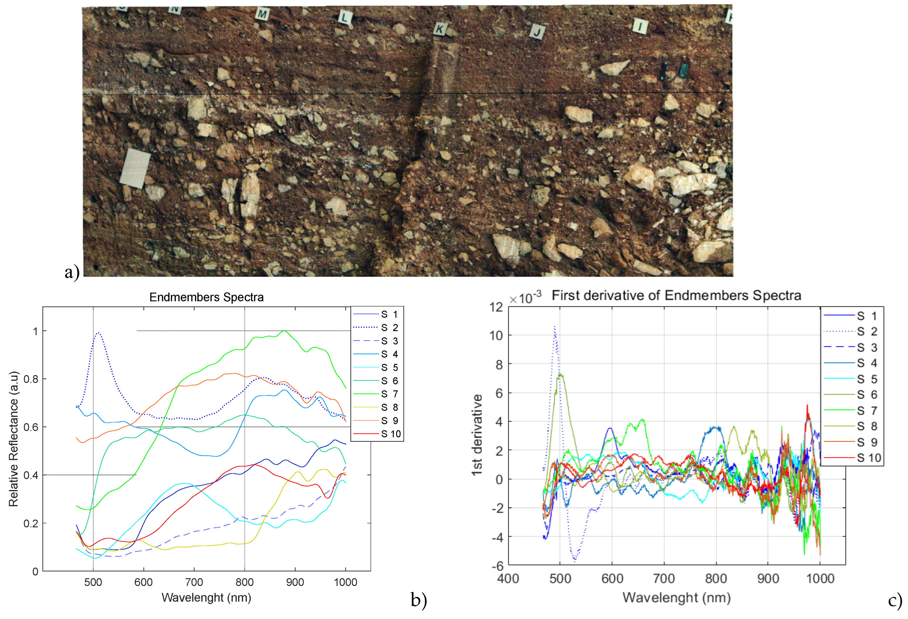
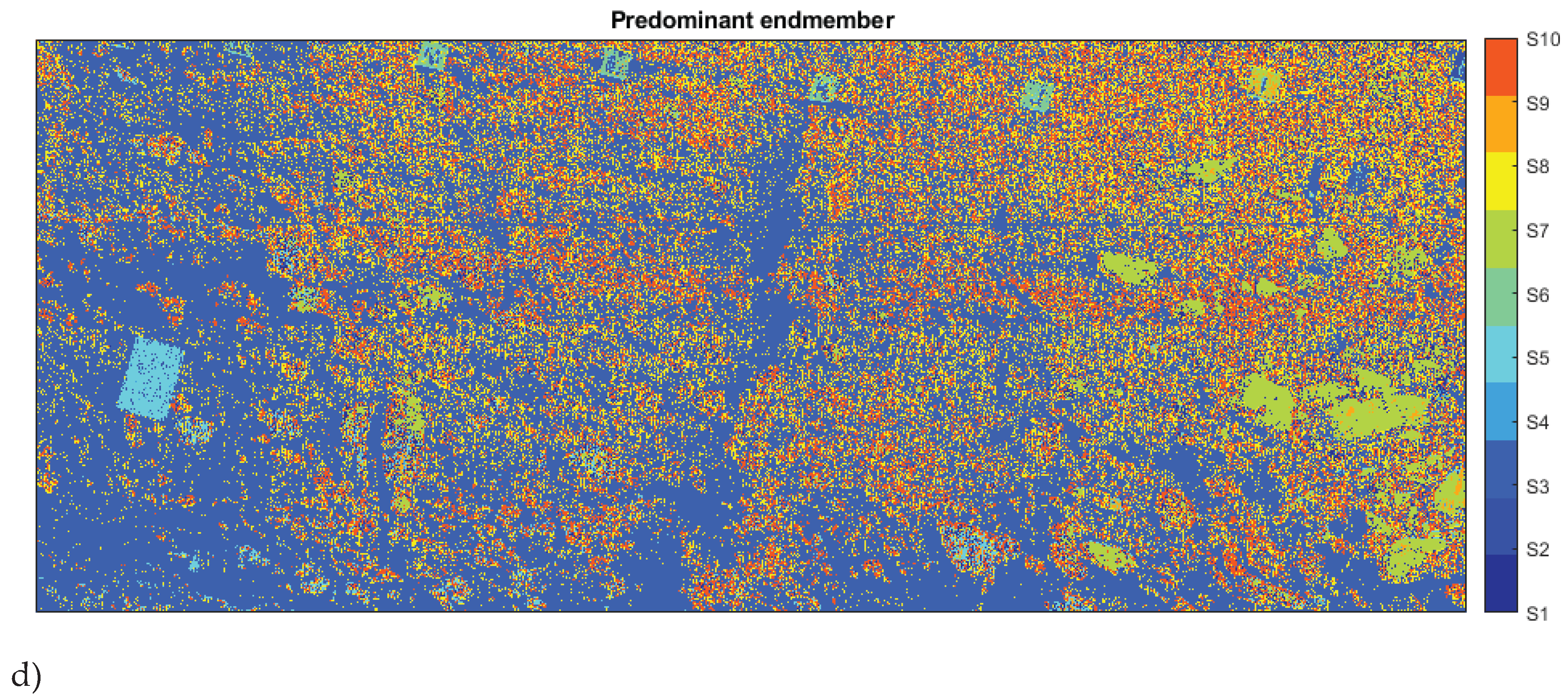
Figure 6.
Spectral abundance map for each endmember (far measurement).
The second column of Table 3 lists the predominant wavelength ranges where spectral peaks are observed, with each peak corresponding to the highest value for each endmember. The third column describes the distribution pattern in the abundance map, which strongly correlates with the surface morphology. Larger materials exhibit greater areas of concentrated abundance (S1, S3, S7), whereas areas with smaller elements demonstrate higher spectral mixing, suggesting a more heterogeneous composition (Figure 5(d)). Notable materials include bones, represented by S2 and S4 in the light blue horizontal lines indicated by arrows. For regions studied, consistent spectral responses were observed, particularly for materials like mud. S8 and S7 show the near-infrared (NIR) response of mud, while S10 reflects an infrared (IR) response. Material degradation varies, influenced by height differences or proximity to more exposed cave surfaces (S10, S3). Additionally, the orientation of the façade impacts material degradation and surface moisture levels (S3). The fourth column lists the primary elements and objects linked to each endmember and their layer and location.
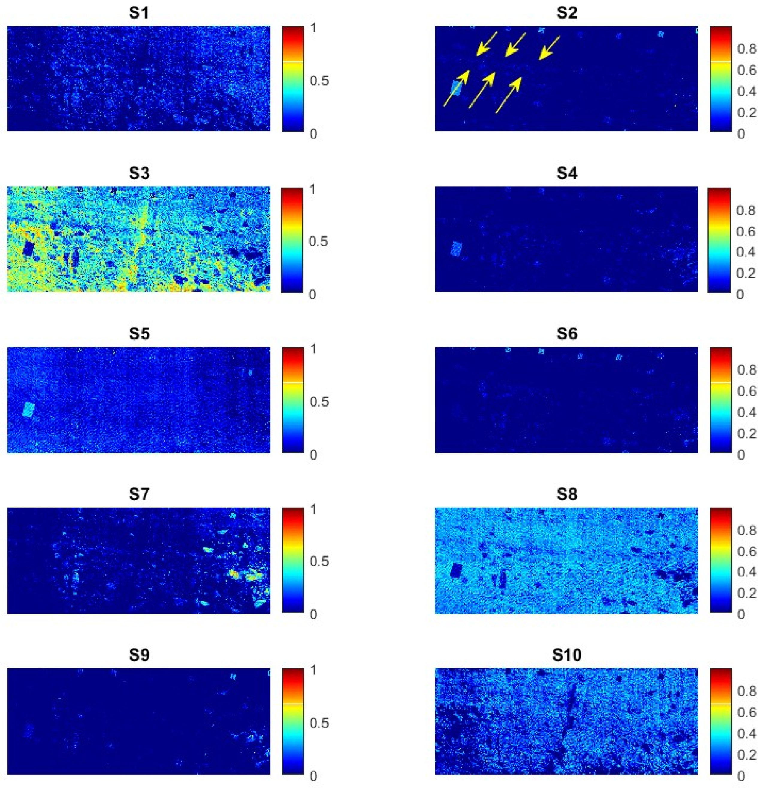
The near HSI response and its processing under indirect lighting conditions are shown in Figure 7 and Figure 8. The highest SAM similarity is observed in Sn7 (91.89%), followed by Sn1 (6.56%) and S3 (1.55%), while the lowest similarity is found in Sn5 (53.90%), Sn6 (22.14%), Sn8 (21.02%), and Sn4 (2.55%) (Figure 7d). Figure 8 illustrates the quantity and spatial distribution of each endmember individually.
Figure 7.
HSI measurements (near). (a) RGB image of the selected study area within the stratigraphic section of the TD10 unit. (b) Spectral signature of each endmember. (c) First derivative of the endmember spectral reflectance. (d) Predominant endmember distribution.
Figure 7.
HSI measurements (near). (a) RGB image of the selected study area within the stratigraphic section of the TD10 unit. (b) Spectral signature of each endmember. (c) First derivative of the endmember spectral reflectance. (d) Predominant endmember distribution.
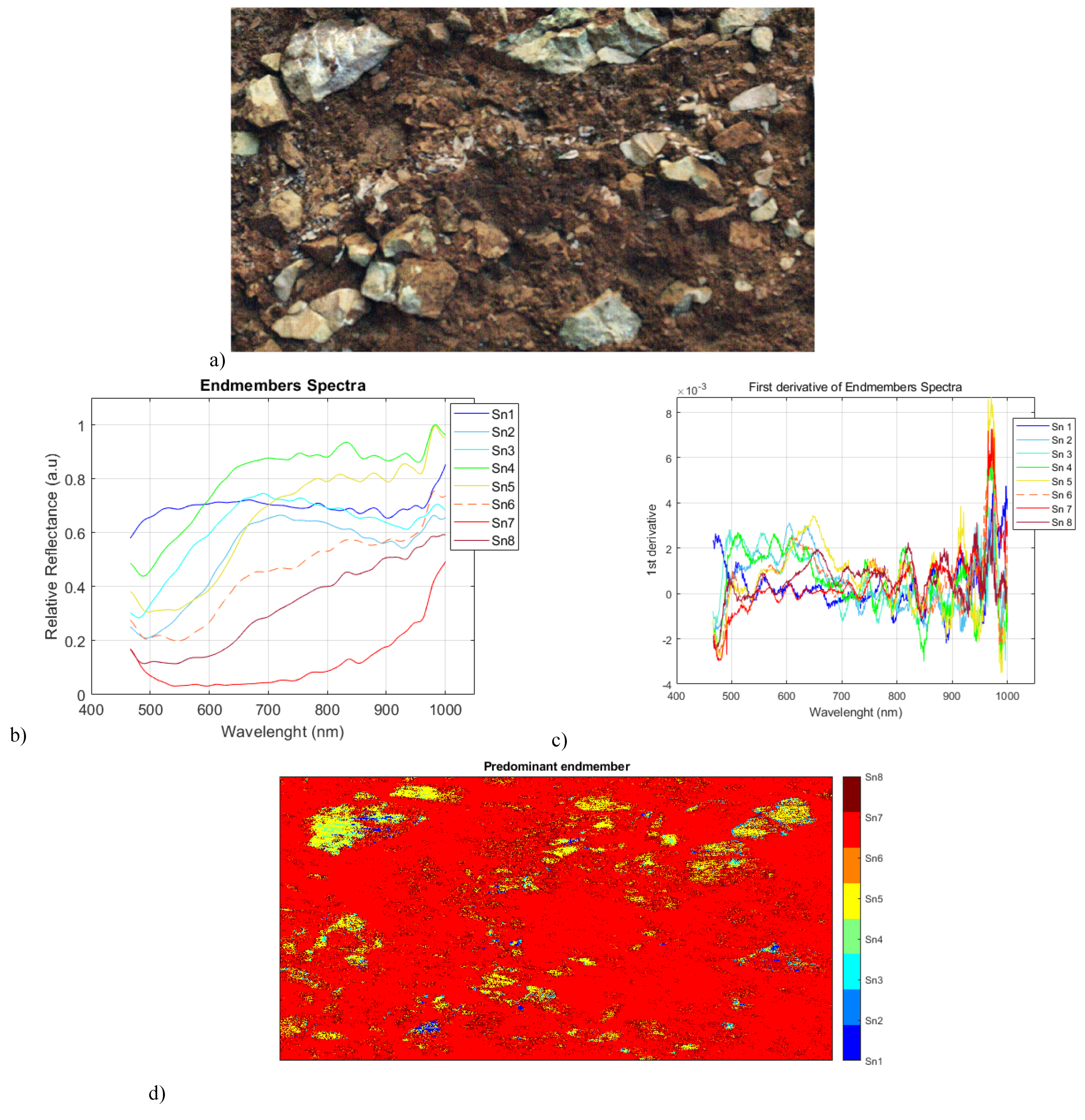
Figure 8.
Spectral abundance maps of each endmember in the near region.
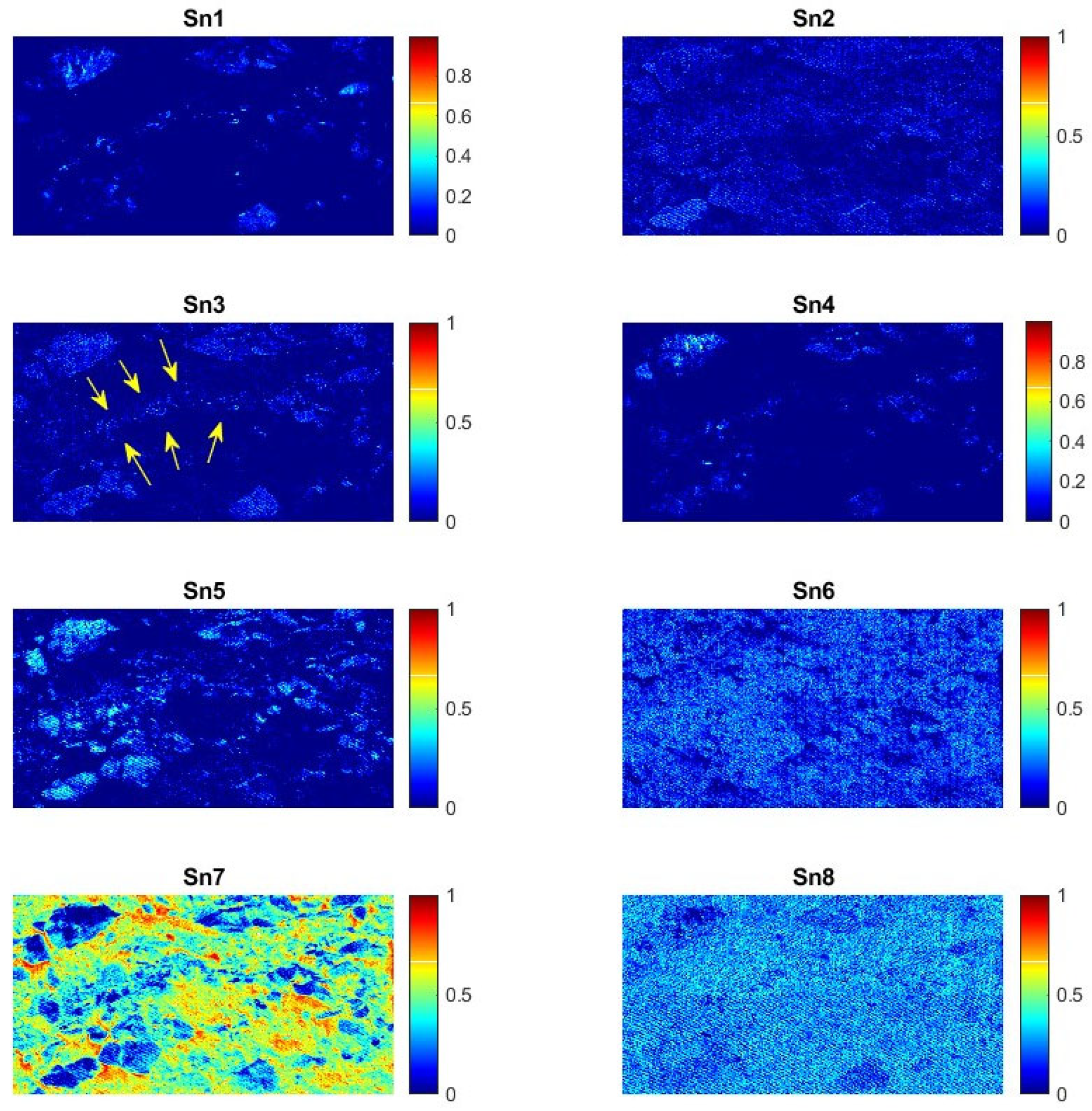
The endmembers detected in the areas containing bones (Sn1, Sn3, and Sn5; see arrows in Figure 8) are mixed with the spectral response of certain stones and limestone. The concentration or dispersion of these endmembers is influenced by the surface's roughness and morphometry. Varying levels of mud detection are observed in Sn2, Sn4, Sn6, and Sn8, while shadows are represented by Sn7 (Table 4).
3.2. Experimental Measurement, Direct Natural Lighting
The analysis under direct natural lighting conditions is performed on two vertical HSI sections of the TD10 unit, labeled A and B (Figure 9a).
Figure 9.
HSI image crop of the stratigraphic section of the TD10 unit, captured under direct natural lighting conditions. (a) RGB image. (b) Spectral signature of each endmember in section A. (c) First derivative of the endmember spectral reflectance in section A. (d) Spectral signature of each endmember in section B. (e) First derivative of the endmember spectral reflectance in section B.
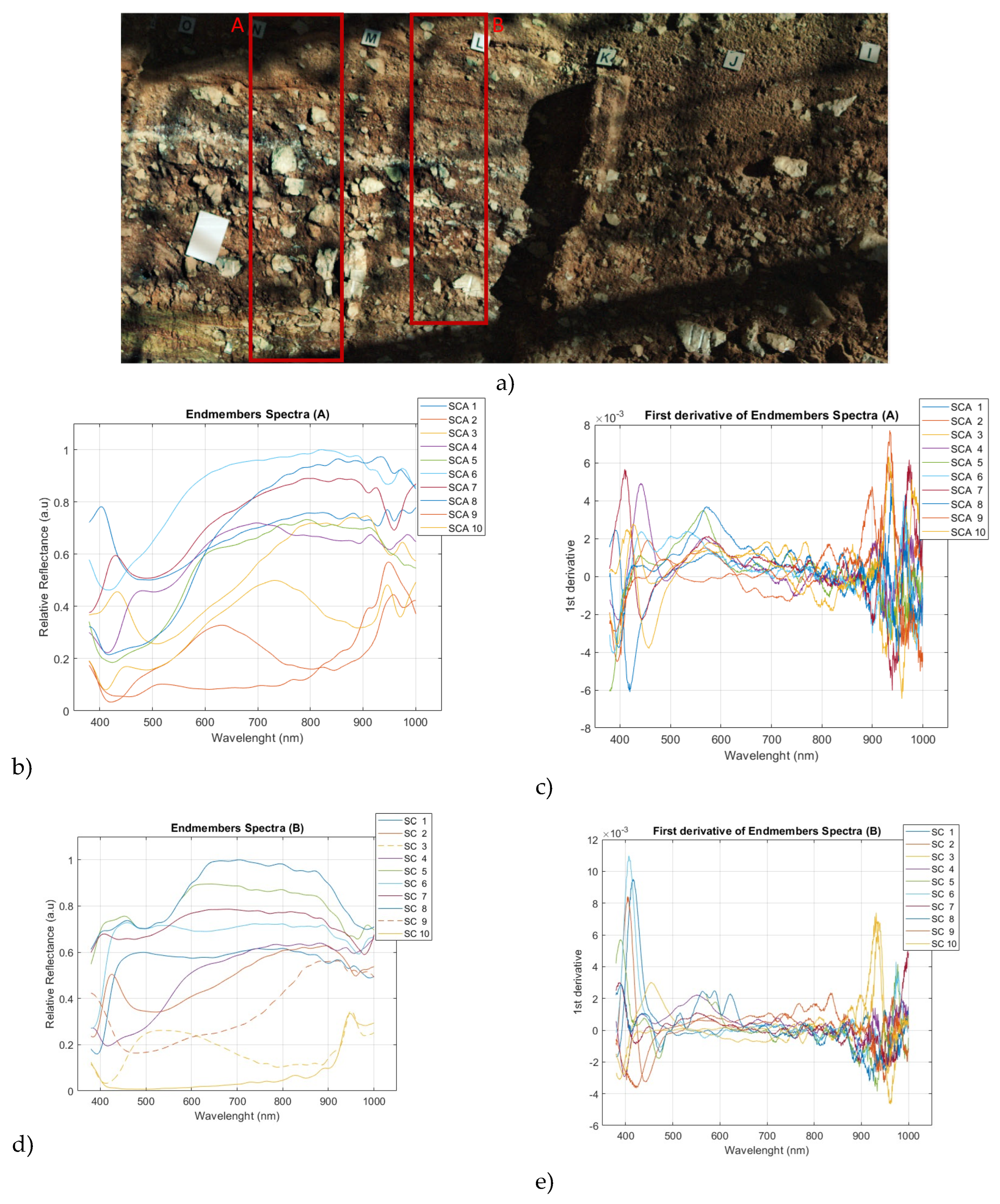
Higher spectral variations are observed in the spectral ranges of 400-500 nm and 850-1000 nm. Additionally, alterations caused by the signal from shadowed areas are detected in the upper left quadrant of Figure 9(d). The abundance map of each endmember is shown in Figure 10, crop A labeled as SCA and crop B labeled as SCB.
Figure 10.
Spectral abundance map of each endmember in the HSI image SCA and SCB (crop A and B), captured under direct natural lighting conditions.
Figure 10.
Spectral abundance map of each endmember in the HSI image SCA and SCB (crop A and B), captured under direct natural lighting conditions.
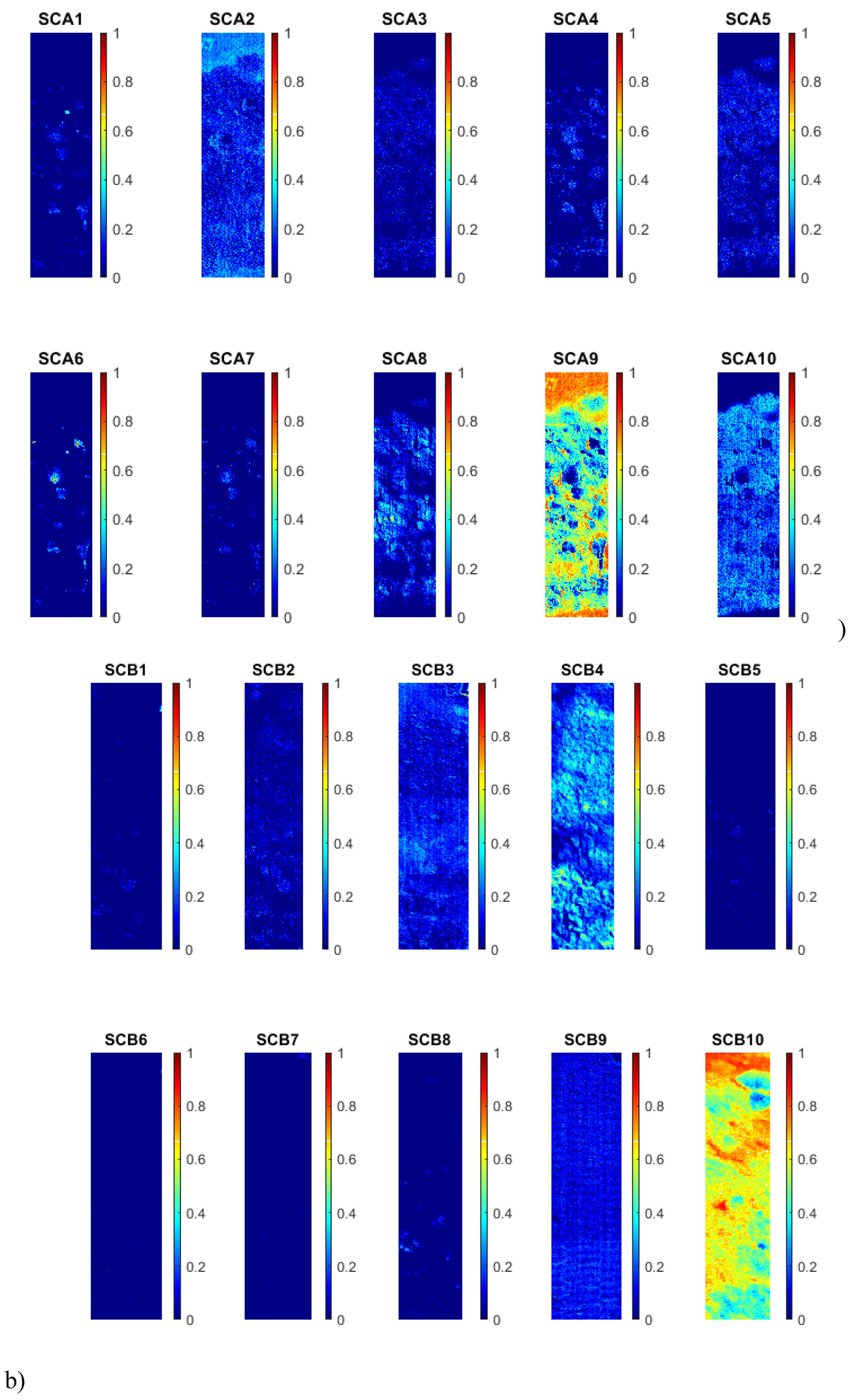
Figure 11 shows the RGB image of crop B (a). The sum of the abundance maps obtained from endmembers SCB4 (brown mud) and SCB10 (dark shadows) allows for the differentiation of the other components and their distribution. This map is presented in a standard color map (b) and a custom color map (c). The custom color map highlights discontinuities and changes in the different layers more distinctly. Two dark, inclined bands with high concentrations are observed, and the arrangement and orientation of the stones are also determined. The abundance map of SCB2 and SCB3 is shown in Figure 11 (d).
4. Discussion and Conclusions
The hyperspectral imaging (HSI) technique has emerged as a powerful analytical tool across various scientific disciplines, enabling the discrimination of distinct quality and spectral attributes. However, its application in the field of geoarchaeology, particularly within Paleolithic sites, has been limited due to specific challenges related to location and environmental conditions. This study presents a straightforward method for measuring and classifying geological and archaeological materials at historic sites, which can facilitate the precise management and characterization of cultural heritage information.
Traditionally, color differences caused by geological changes have been evaluated through visual perception. In contrast, HSI provides more precise data. Previous analyses of the southeast stratigraphic TD10 unit at Gran Dolina, based on the Munsell Soil Color Chart, identified three distinct color varieties within the photopic visual range (380-780 nm): yellowish red 5YR 5/8, reddish yellow 5YR 6/8, and reddish yellow 5YR 7/8, as detailed in Table 2. This work assesses spectral reflectance differences through several predominant spectral endmembers that have been automatically identified. The proportion of each pixel containing these endmembers has been calculated (see Figure 6, Figure 8, and Figure 10), allowing for accurate identification of the spectral concentration and distribution of elements and sediments. While visual evaluation can be influenced by factors such as the characteristics of the observer’s visual system and the illumination used, HSI methodology provides a consistent statistical classification that enhances precision, even in response to variations in the lighting system. This approach enables the differentiation of similar elements that may appear identical or nearly so to the naked eye. Notably, spectral detection in the near-infrared (NIR) range is impossible to achieve without HSI; however, this technique captures spectral responses in the NIR range effectively.
The analysis and processing of HSI data facilitate the spectral characterization of representative elements and their spatial distributions through endmember identification. Additionally, the use of spectral derivatives enhances classification and improves resolution, aiding in the identification and separation of individual spectral contributions. Results indicate that measurements obtained under direct illumination exhibit more stable values in the central part of the spectral range, while extreme ends show high slopes.
The resulting abundance maps reveal discontinuities and accumulations based on spectral and spatial distributions. Utilizing both local and global probabilities for mixed pixel characterization enables qualitative and quantitative evaluations. Results obtained from far-field measurements demonstrate a capacity to discriminate more uniform distributions, aligning well with prior field observations. Conversely, the spectral abundance map derived from close-distance measurements delineates a well-defined zone adjacent to the archaeological and paleoanthropological stratigraphic deposits. Moreover, independent processing of spectral reflectance for each endmember highlights differences, similarities, and material accumulations. A horizontal line visible in the upper center of the image (Figures 6, S2; 8, S1, S3) corresponds to bone remains. Spatial distributions linked to the blue spectral range (Figure 6: S1) and the NIR (Figure 6: S8) are not discernible in the RGB image. Several factors, including humidity and degradation from exposure to the elements (Figure 6: S3), or material displacement due to handling, contribute to blurring in the data.
The close-up images provide a clearer identification of blocks (Sn5), except where stained by the surrounding matrix, which appears relatively uniform (mostly Sn7). Classes Sn1 and Sn3 exhibit a blue tendency associated with stones and bones. Direct natural lighting analysis facilitates the differentiation of smaller areas. Increased light intensity permits the evaluation of minor variations; however, the solar incidence angle can introduce shadows due to surface roughness, inclination, and infrastructural obstructions.
Variations in lighting conditions, image resolution, and area size during far and near-field measurements enable the characterization of different landscape mosaics, revealing principal color textures and material types. HSI analysis opens new avenues for research, enhancing the existing database of archaeological and paleoanthropological stratigraphic deposits. Future studies will provide opportunities for deeper explorations of topographic comparisons.
The hyperspectral analysis reveals significant spectral variations in the 400-500 nm and 850-1000 nm ranges, highlighting key differences in material composition. Shadow-induced alterations affect signal interpretation, emphasizing the need to consider lighting conditions in the analysis. The distribution of different materials is effectively mapped, allowing for a clearer differentiation of components. Additionally, the use of a custom color map enhances the visualization of layer discontinuities and structural patterns, such as the orientation of stones and the presence of high-concentration bands. These findings demonstrate the effectiveness of hyperspectral imaging in improving the characterization of geological and sedimentary structures.
In summary, the experimental HSI measurement procedures conducted at Gran Dolina cave in Atapuerca (Sierra de Atapuerca, Burgos, Spain), coupled with subsequent data processing, have facilitated the hyperspectral characterization of diverse elements and materials from the TD10 sediment. This study outlines a comprehensive exploration method that includes experimental data collection, supervised statistical classification, and spectral derivative processes for both far and near-field analyses.
Overall, the findings highlight the significant characteristics of stratigraphic information derived from endmember extraction techniques applied to hyperspectral data, in accordance with the statistical classification methods used to compare image spectra under varying illumination conditions. Data processing encompasses both global and local classifications within the predominant spectrum, including the NIR spectrum, which is undetectable by human vision or conventional cameras. This spectral classification enables spatial quantification and differentiation of significant responses. The hyperspectral assessment of archaeological and paleoanthropological stratigraphic deposits serves as a potent digital resource, contributing to the sustainable management of Cultural Heritage information and enhancing Environmental Sciences.
The hyperspectral imaging (HSI) assessment of archaeo-paleoanthropological stratigraphic deposits at Atapuerca, as presented in this study, underscores the increasing relevance of HSI in cultural heritage and paleoanthropological research. The proposed methodology, which integrates HSI measurements with statistical classification techniques, aligns with the broader applications of hyperspectral imaging in the cultural heritage field. Furthermore, the Atapuerca study highlights the importance of spectral models for material classification emphasizing the role of machine learning in the study of deposits within cultural heritage research. By leveraging HSI for the digital characterization of stratigraphic deposits, this research not only contributes to human evolution studies but also supports sustainable management practices, reinforcing the potential of HSI as a fundamental tool in both archaeological and heritage science.
Author Contributions
Conceptualization, B.G.-F. and A.B.-C.; data capture and methodology, B.G.-F.; A.B-C.; A.M.-F.; project administration, B.G-F. and A.B-C.; software, B.G.-F and A. B.-C.; validation, B.G.-F., A.B.-C., A.M.-F. and I.C.; formal analysis, B.G.-F.; investigation, B.G.-F., A.B.-C., A.M.-F., I.C.; resources, B.G.-F., A.B.-C., A.M.-F., I.C.; writing—original draft preparation, B.G.-F and I.C.; writing—review and editing, B.G.-F., A.B.-C., A.M.-F., I.C.; A.O., P.S., M.M.-T., M.M.; visualization, B.G.-F., A.B.-C., A.M.-F., I.C.; supervision, A.O., P.S., M.M.-T., M.M.;. All authors have read and agreed to the published version of the manuscript.
Acknowledgments
The authors would like to acknowledge the financial support received from Universidad Politécnica de Madrid, Spain. This study was supported by the project PID2021-122355NB-C33 financed by MCIN/ AEI/10.13039/501100011033/ FEDER, UE. The results of this study are supported by research by Berta García Fernández who carried out a research stay between June and August 2022 (three months) in the Spanish National Research Center for Human Evolution (CENIEH). Hyperspectral capture was carried out with VNIR A Series Headwall Photonics camera, available at the Laboratory of Digital Mapping & 3D Analysis (CENIEH). We thank the EIA, and TD10 excavation team and its coordinators, A. Ollé and P. Saladié.
Conflicts of Interest
The authors declare no conflict of interest.
References
- Pavia, D. L., et al. Introduction to spectroscopy. Cengage Learning, 2014.
- Saha, D., & Manickavasagan, A. (2021). Machine learning techniques for analysis of hyperspectral images to determine quality of food products: A review. Current Research in Food Science, 4, 28-44. [CrossRef]
- d’Oleire-Oltmanns, S., Marzolff, I., Peter, K. D., & Ries, J. B. (2012). Unmanned aerial vehicle (UAV) for monitoring soil erosion in Morocco. Remote Sensing, 4(11), 3390-3416. [CrossRef]
- Miřijovský, J., Langhammer, J. Multitemporal monitoring of the morphodynamics of a mid-mountain stream using UAS photogrammetry. Remote Sensing. 2015;7(7):8586-609. [CrossRef]
- Gomez, C., Purdie, H. UAV-based Photogrammetry and Geocomputing for Hazards and Disaster Risk Monitoring–A Review. Geoenvironmental Disasters. 2016;3(1):23. [CrossRef]
- Adão, T., Hruška, J., Pádua, L., Bessa, J., Peres, E., Morais, R., & Sousa, J. J. (2017). Hyperspectral imaging: A review on UAV-based sensors, data processing and applications for agriculture and forestry. Remote Sensing, 9(11), 1110. [CrossRef]
- Asner, G. P., Wessman, C. A., Bateson, C. A., & Privette, J. L. (2000). Impact of tissue, canopy, and landscape factors on the hyperspectral reflectance variability of arid ecosystems. Remote Sensing of Environment, 74(1), 69-84. [CrossRef]
- Transon, J., d’Andrimont, R., Maugnard, A., & Defourny, P. (2018). Survey of hyperspectral earth observation applications from space in the sentinel-2 context. Remote Sensing, 10(2), 157. [CrossRef]
- Urbanos, G., Martín, A., Vázquez, G., Villanueva, M., Villa, M., Jimenez-Roldan, L., & Sanz, C. (2021). Supervised Machine Learning Methods and Hyperspectral Imaging Techniques Jointly Applied for Brain Cancer Classification. Sensors, 21(11), 3827. [CrossRef]
- Fischer, C., & Kakoulli, I. (2006). Multispectral and hyperspectral imaging technologies in conservation: current research and potential applications. Studies in Conservation, 51(sup1), 3-16. [CrossRef]
- Picollo, M., Cucci, C., Casini, A., & Stefani, L. (2020). Hyper-spectral imaging technique in the cultural heritage field: New possible scenarios. Sensors, 20(10), 2843. [CrossRef]
- Jacq, K., Debret, M., Fanget, B., Coquin, D., Sabatier, P., Pignol, C., ... & Perrette, Y. (2022). Theoretical Principles and Perspectives of Hyperspectral Imaging Applied to Sediment Core Analysis. Quaternary, 5(2), 28. [CrossRef]
- Linderholm, J., Geladi, P., Gorretta, N., Bendoula, R., & Gobrecht, A. (2019). Near infrared and hyperspectral studies of archaeological stratigraphy and statistical considerations. Geoarchaeology, 34(3), 311-321. [CrossRef]
- Doneus, M., Verhoeven, G., Atzberger, C., Wess, M., & Ruš, M. (2014). New ways to extract archaeological information from hyperspectral pixels. Journal of Archaeological Science, 52, 84-96. [CrossRef]
- Guanter, L., Richter, R., & Moreno, J. (2006). Spectral calibration of hyperspectral imagery using atmospheric absorption features. Applied optics, 45(10), 2360-2370. [CrossRef]
- Peyghambari, S., & Zhang, Y. (2021). Hyperspectral remote sensing in lithological mapping, mineral exploration, and environmental geology: an updated review. Journal of Applied Remote Sensing, 15(3), 031501-031501. [CrossRef]
- Ortega, A. I., Benito-Calvo, A., Pérez-González, A., Martín Merino, M. A., Pérez-Martínez, R., Parés, J. M., Aramburu, A., Arsuaga, J. L., Bermúdez de Castro, J. M., & Carbonell, E. (2013). Evolution of multilevel caves in the Sierra de Atapuerca (Burgos, Spain) and its relation to human occupation. Geomorphology, 196, 122–137. [CrossRef]
- Ortega, A. I., Benito-Calvo, A., Martín, M.A., Pérez-González, A., Parés, J. M., Bermúdez de Castro, J. M., Arsuaga, J. L., & Carbonell, E. (2018). Las cuevas de la Sierra de Atapuerca y el uso del paisaje kárstico durante el Pleistoceno (Burgos, España). Boletín Geológico y Minero, 129(1), 083–106. [CrossRef]
- Benito-Calvo, A., & Pérez González, A. (2015). Geomorphology of the Sierra de Atapuerca and the Middle Arlanzón Valley (Burgos, Spain). Journal of Maps, 11(4), 535–544. [CrossRef]
- Benito-Calvo, A., Ortega, A. I., Navazo, M., Moreno, D., Pérez-Gonzalez, A., Parés, J. M., Bermúdez De Castro, J. M., & Carbonell, E. (2018). Pleistocene geodynamic evolution of the Arlanzón valley: Implications for the formation of the endokarst system and the open air archaeological sites of the Sierra de Atapuerca (Burgos, España). Boletín Geológico y Minero, 129(1), 059–082. [CrossRef]
- Picollo, M., Cucci, C., Casini, A., & Stefani, L. (2020). Hyper-spectral imaging technique in the cultural heritage field: New possible scenarios. Sensors, 20(10), 2843. [CrossRef]
- Campaña, I., Benito-Calvo, A., Pérez-González, A., Ortega, A.I., Bermúdez De Castro, J.M., Carbonell, E., 2016. Using 3D models to analyse stratigraphic and sedimentological contexts in archaeo-palaeo-anthropological Pleistocene sites (Gran Dolina site, Sierra de Atapuerca), in: Campana, S., Scopigno, R., Carpentiero, G., Cirillo, M. (Eds.), CAA 2015 KEEP THE REVOLUTION GOING. Proceedings of the 43rd Annual Conference on Computer Applications and Quantitative Methods in Archaeology. Archeopress, Oxford, pp. 337–345.
- Campaña, I., Benito-Calvo, A., Pérez-González, A., Ortega, A. I., Bermúdez de Castro, J. M., & Carbonell, E. (2017). Pleistocene sedimentary facies of the Gran Dolina archaeo-paleoanthropological site (Sierra de Atapuerca, Burgos, Spain). Quaternary International, 433, 68-84. [CrossRef]
- Campaña, I. (2018). Estratigrafía y sedimentología del yacimiento de Gran Dolina (Sierra de Atapuerca, Burgos). Ph.D Thesis. University of Burgos, Spain. [CrossRef]
- Martínez-Fernández, A., Benito-Calvo, A., Campaña, I., Ortega, A. I., Karampaglidis, T., de Castro, J. M. B., & Carbonell, E. (2020). 3D monitoring of Paleolithic archaeological excavations using terrestrial laser scanner systems (Sierra de Atapuerca, Railway Trench sites, Burgos, N Spain). Digital Applications in Archaeology and Cultural Heritage, 19, e00156. [CrossRef]
- Bermúdez de Castro, J.M., Arsuaga, J.L., Carbonell, E., Rosas, A., Martínez, I., Mosquera, M., 1997. A Hominid from the lower Pleistocene of Atapuerta, Spain: possible ancestor to Neandertals and modern humans. Science 276, 1392–1395. . [CrossRef]
- Carbonell, E., Bermúdez de Castro, J.M., Parés, J.M., Pérez-González, A., Cuenca-Bescos, G., Ollé, A., Mosquera, M., Huguet, R., Made, J. van der, Rosas, A., Sala, R., Vallverdú, J., García, N., Granger, D.E., Martinón-Torres, M., Rodríguez, X.P., Stock, G.M., Vergès, J.M., Allué, E., Burjachs, F., Cáceres, I., Canals, A., Benito, A., Díez, C., Lozano, M., Mateos, A., Navazo, M., Rodríguez, J., Rosell, J., Arsuaga, J.L., 2008. The first hominin of Europe. Nature 452, 465–469. [CrossRef]
- Ollé, A., Mosquera, M., Rodríguez, X.P., de Lombera-Hermida, A., García-Antón, M.D., García-Medano, P., Peña, L., Menéndez, L., Navazo, M., Terradillos, M., Bargalló, A., Márquez, B., Sala, R., Carbonell, E., 2013. The Early and Middle Pleistocene technological record from Sierra de Atapuerca (Burgos, Spain). Quaternary International 295, 138–167. [CrossRef]
- Rodríguez, J., Burjachs, F., Cuenca-Bescós, G., García, N., Van der Made, J., Pérez González, A., Blain, H-A., Expósito, I., López-García, J.M., García Antón, M., Allué, E., Cáceres, I., Huguet, R., Mosquera, M., Ollé, A., Rosell, J., Parés, J.M., Rodríguez, X.P., Díez, C., Rofes, J., Sala, R., Saladié, P., Vallverdú, J., Bennasar, M.L., Blasco, R., Bermúdez de Castro, J.M., Carbonell, E., 2011. One million years of cultural evolution in a stable environment at Atapuerca (Burgos, Spain). Quaternary Science Reviews 30 (11-12), 1396-1412. [CrossRef]
- Ortega, A. I., Benito-Calvo, A., Pérez-González, A., Martín Merino, M. A., Pérez-Martínez, R., Parés, J. M., Aramburu, A., Arsuaga, J. L., Bermúdez de Castro, J. M., & Carbonell, E. (2013). Evolution of multilevel caves in the Sierra de Atapuerca (Burgos, Spain) and its relation to human occupation. Geomorphology, 196, 122–137. [CrossRef]
- Benito-Calvo, A., Ortega, A. I., Pérez-González, A., Campaña, I., Bermúdez de Castro, J. M., & Carbonell, E. (2017). Palaeogeographical reconstruction of the Sierra de Atapuerca Pleistocene sites (Burgos, Spain). Quaternary International, 433, 379–392. [CrossRef]
- Moreno, D., Falguères, C., Pérez-González, A., Duval, M., Voinchet, P., Benito-Calvo, A., Ortega, A. I., Bahain, J. J., Sala, R., Carbonell, E., Bermúdez de Castro, J. M., & Arsuaga, J. L. (2012). ESR chronology of alluvial deposits in the Arlanzón valley (Atapuerca, Spain): Contemporaneity with Atapuerca Gran Dolina site. Quaternary Geochronology, 10, 418–423. [CrossRef]
- Gil, E., Aguirre, E., Hoyos, M., 1987. Contexto Estratigráfico. In: Aguirre, E., Carbonell, E., Bermúdez de Castro, J.M. El hombre fósil de Ibeas y el Pleistoceno de la Sierra de Atapuerca. Ed. Junta de Castilla y León.
- Ortega Martínez, A.I., Ruiz García, F., Benito Calvo, A., Martín Merino, M.A., Karampaglidis, T., Campaña Lozano, I., 2014. Escaneado en 3D de las Galerías de las Huellas. Cubía 18, 38–48.
- Pérez-González, A., Parés, J.M., Carbonell, E., Aleixandre, T., Ortega, A.I., Benito, A., Martín, M.A., 2001a. Géologie de la Sierra de Atapuerca et stratigraphie des remplissages karstiques de Galería et Dolina (Burgos, Espagne). L ́Anthropologie 105, 27–43. [CrossRef]
- Parés, J.M., Arnold, L., Duval, M., Demuro, M., Pérez-González, A., Bermúdez de Castro, J.M., Carbonell, E., Arsuaga, J.L., 2013. Reassessing the age of Atapuerca-TD6 (Spain): New paleomagnetic results. Journal of Archaeological Science 40, 4586–4595. [CrossRef]
- Moreno, D., Falguères, C., Pérez-González, A., Voinchet, P., Ghaleb, B., Despriée, J., Bahain, J.-J., Sala, R., Carbonell, E., Bermúdez de Castro, J.M., Arsuaga, J.L., 2015. New radiometric dates on the lowest stratigraphical section (TD1 to TD6) of Gran Dolina site (Atapuerca, Spain). Quaternary Geochronology 30, 535–540. [CrossRef]
- HEADWALL PHOTONICS, Inc. Hyperspectral Imaging Sensors: Hyperspec VNIR [online 01/11/2022]. Available from: https://www.headwallphotonics.com/products/vnir-400-1000nm.
- Kale, K. V., Solankar, M. M., Nalawade, D. B., Dhumal, R. K., & Gite, H. R. (2017). A research review on hyperspectral data processing and analysis algorithms. Proceedings of the national academy of sciences, India section a: physical sciences, 87(4), 541-555. [CrossRef]
- Polder, G., van der Heijden, G. W., Keizer, L. P., & Young, I. T. (2003). Calibration and characterisation of imaging spectrographs. Journal of Near Infrared Spectroscopy, 11(3), 193-210. [CrossRef]
- Chang, Chein-I., and Qian Du. "Estimation of number of spectrally distinct signal sources in hyperspectral imagery." IEEE Transactions on geoscience and remote sensing 42, no. 3 (2004): 608-619. [CrossRef]
- M.E. Winter, N-FINDR: an algorithm for fast autonomous spectral end-member determination in hyperspectral data, Proc. SPIE 3753, Imaging Spectrometry V, 1999. [CrossRef]
- Debba, P., Carranza, E. J., van der Meer, F. D., & Stein, A. (2006). Abundance estimation of spectrally similar minerals by using derivative spectra in simulated annealing. IEEE transactions on geoscience and remote sensing, 44(12), 3649-3658. [CrossRef]
- F. A. Kruse, A. B. Lefkoff, J. W. Boardman, K. B. Heidebrecht, A. T. Shapiro, P. J. Barloon, and A. F. H. Goetz, "The Spectral Image Processing System (SIPS) Interactive Visualization and Analysis of Imaging Spectrometer Data," Remote Sens. Environ., vol. 44, no. 2-3, pp. 145-163, May-Jun. 1993. [CrossRef]
- Kay, S. M. (1993). Fundamentals of statistical signal processing: estimation theory. Prentice-Hall, Inc.
- Somers, B., Asner, G. P., Tits, L., & Coppin, P. (2011). Endmember variability in spectral mixture analysis: A review. Remote Sensing of Environment, 115(7), 1603-1616. [CrossRef]
Figure 1.
Sedimentary facies of Gran Dolina southeast Stratigraphic TD10 level [23].
Figure 1.
Sedimentary facies of Gran Dolina southeast Stratigraphic TD10 level [23].
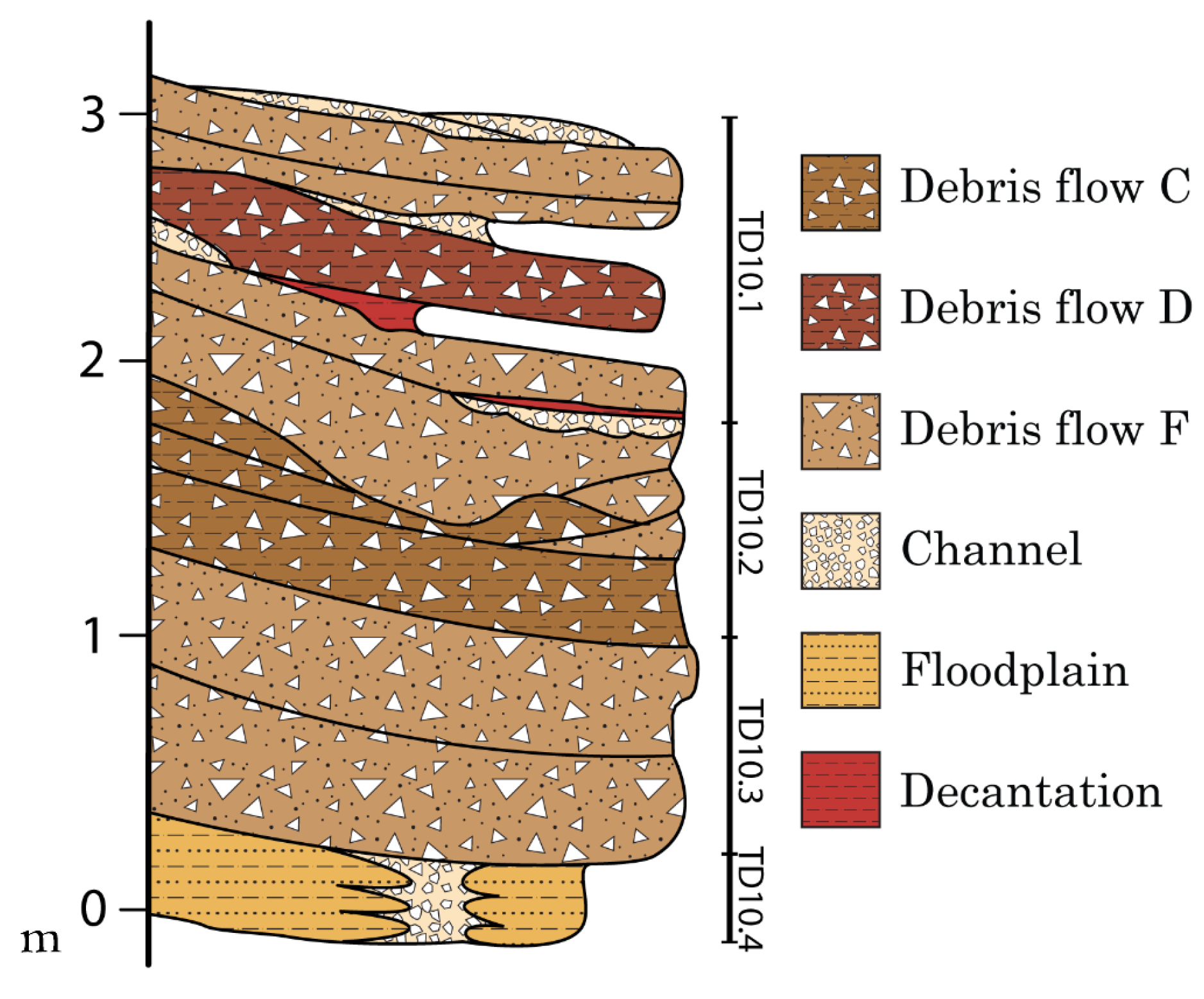
Figure 2.
a) Measurement area location of experimental setup carried out in Gran Dolina cave on Atapuerca (Sierra de Atapuerca. b) Sedimentary facies described in TD10. Black lines indicate stratigraphic limits [24].
Figure 2.
a) Measurement area location of experimental setup carried out in Gran Dolina cave on Atapuerca (Sierra de Atapuerca. b) Sedimentary facies described in TD10. Black lines indicate stratigraphic limits [24].
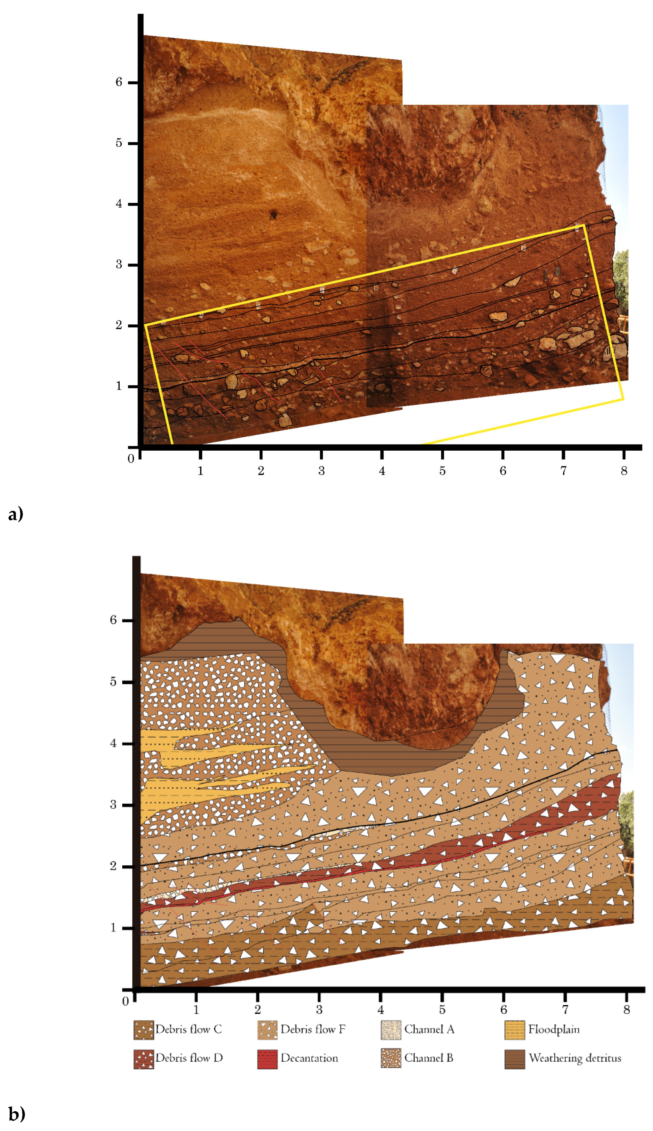
Figure 3.
(a) The Gran Dolina cave at Atapuerca (Sierra de Atapuerca, Burgos, Spain), experimental setup.
Figure 3.
(a) The Gran Dolina cave at Atapuerca (Sierra de Atapuerca, Burgos, Spain), experimental setup.
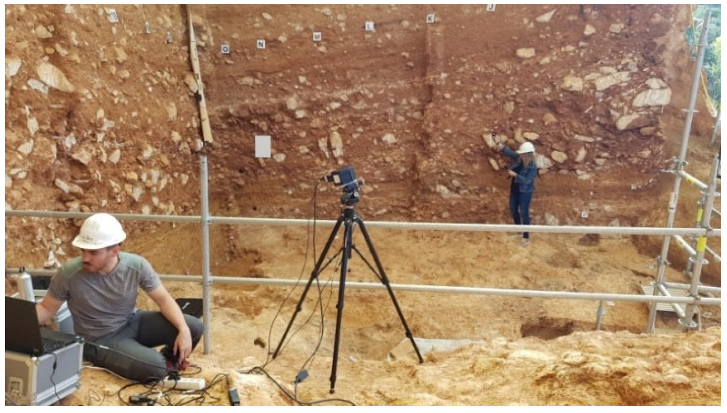
Figure 4.
(a) Aerial view of Atapuerca sites, (Sierra de Atapuerca, Burgos, Spain): Gran Dolina cave, marked with the number 1 in red color. Satellite view: Sun path diagram of the site (b) June and (c) August 22. (d) Sun path diagram of the site on August 22 2022.
Figure 4.
(a) Aerial view of Atapuerca sites, (Sierra de Atapuerca, Burgos, Spain): Gran Dolina cave, marked with the number 1 in red color. Satellite view: Sun path diagram of the site (b) June and (c) August 22. (d) Sun path diagram of the site on August 22 2022.
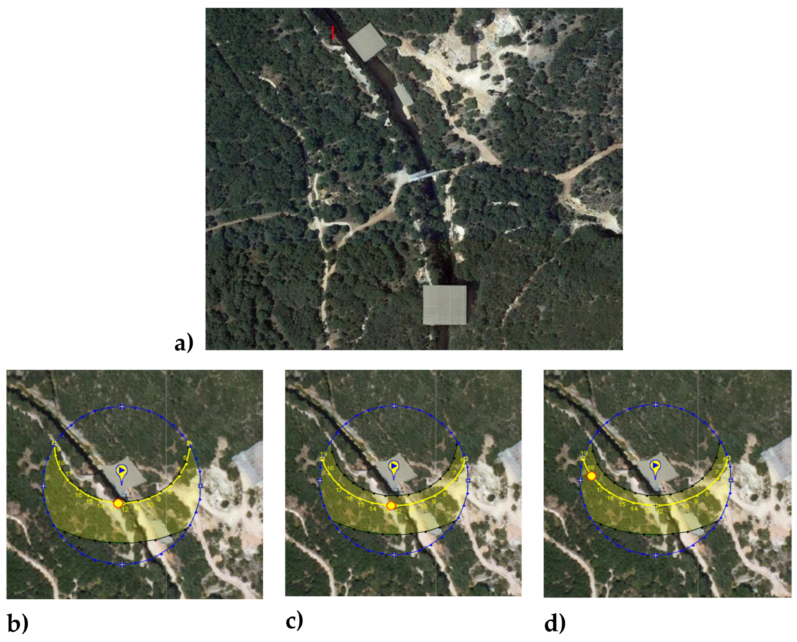
Figure 11.
(a) The RGB image of B (b) SCB4 plus SCB10, (c) SCB4 plus SCB10, (d) SCB2 plus SCB3.
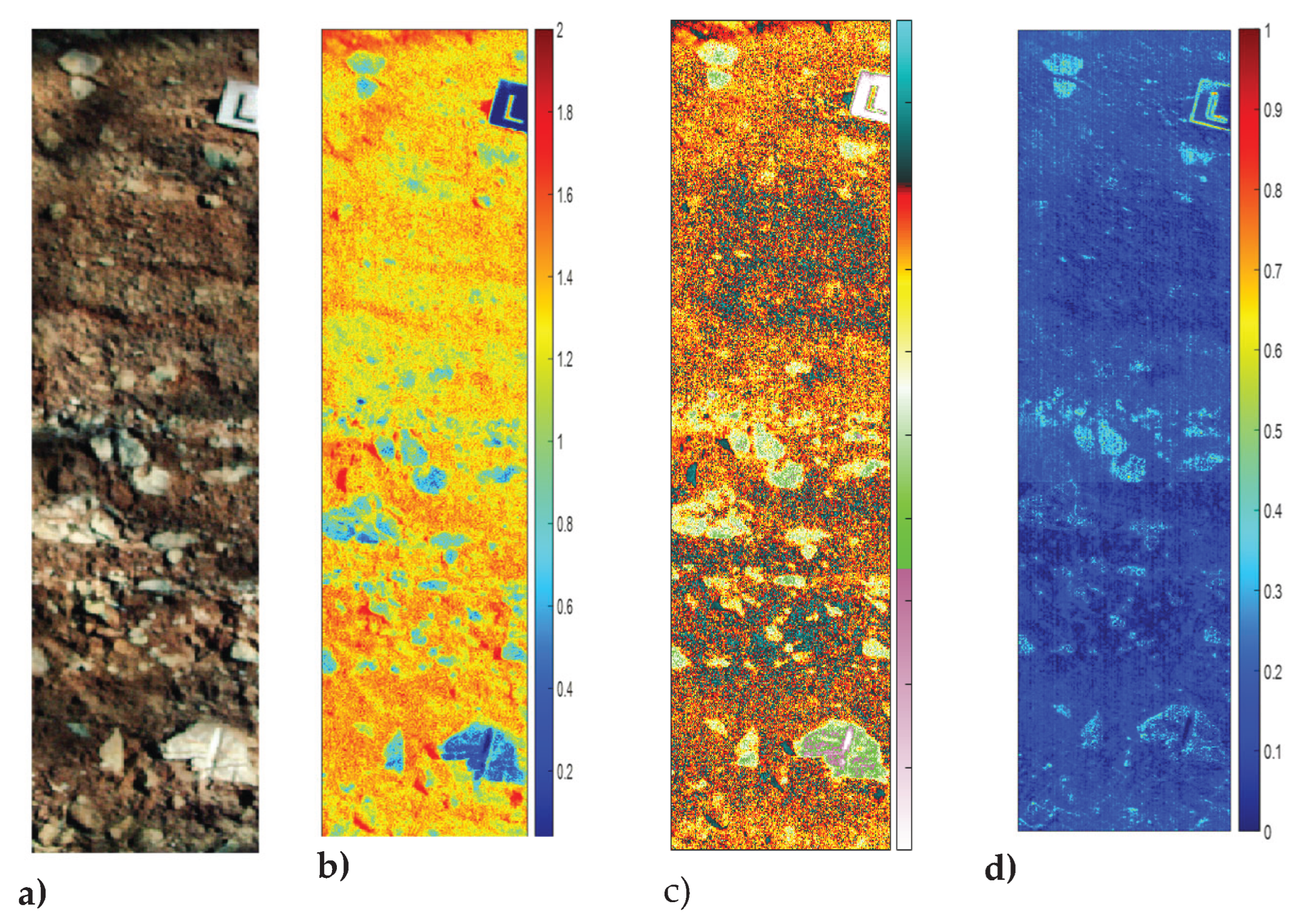

Table 1.
Brief description of the sedimentary facies of TD10 [22].
Table 1.
Brief description of the sedimentary facies of TD10 [22].
| Facies | Brief description |
|---|---|
| Debris flow C | Clast‐supported boulders with muddy matrix |
| Debris flow D | Matrix-supported boulders and gravels with muddy matrix |
| Debris flow F | Grain-supported boulders |
| Channel | Grain-size decreasing gravels |
| Floodplain | Silts and clays |
| Decantation | Clayey silts |
Table 2.
Sedimentary facies of TD10 according to the Munsell soil color chart.
| Sub-unit | Layer | Thick (cm) | Facies | Color |
| TD10.1 | 1 | 18 | Channel | Yellowish red 5YR 5/8 |
| 2 | 25 | Debris flow F | Reddish yellow 5YR 6/8 | |
| 3 | 20 | Debris flow F | Reddish yellow 5YR 6/8 | |
| 4 | 15 | Channel | Reddish yellow 5YR 6/8 | |
| 5 | 30 | Debris flow D | Yellowish red 5YR 5/8 | |
| 6 | 25 | Decantation | Yellowish red 5YR 5/6 | |
| 7 | 25 | Debris flow F | Reddish yellow 5YR 6/8 | |
| TD10.2 | 1 | 15 | Channel / Decantation | Reddish yellow 5YR 6/8 |
| 2 | 45 | Debris flow F | Reddish yellow 5YR 6/8 | |
| 3 | 35 | Debris flow C | Yellowish red 5YR 5/8 | |
| 4 | 20 | Debris flow F | Reddish yellow 5YR 6/8 | |
| 5 | 30 | Debris flow F | Reddish yellow 5YR 6/8 | |
| 6 | 50 | Debris flow C | Strong brown 7.5YR 5/6 | |
| TD10.3 | 1 | 35 | Debris flow F | Reddish yellow 5YR 6/8 |
| 2 | 45 | Debris flow F | Reddish yellow 5YR 6/8 | |
| TD10.4 | 1 | 30 | Channel / Floodplain / Decantation | Yellowish red 5YR 5/8 |
Table 3.
Sedimentary characteristics of TD10 based on endmember classification (far region).
| Endmember | Predominant Spectrum- (Spectral peak) |
Surface Morphology | Sediment/object | Main location |
|---|---|---|---|---|
| S1 | Orange-Red+IR (Peak 950 nm) |
Uniform, Irregular, decreasing, |
Mud | TD10 Higher in upper right |
| S2 | Bluish-Red+IR (Peak 510 nm) |
Scattered | Bones, Small stones, gravels, reference targets |
TD10 Middle & bottom |
| S3 | Reddish-brown (Peak 1000 nm) |
Uniform, increasing | Mud | TD10, higher in lower left & central vertical line |
| S4 | Bluish-white-NIR (Peak 950 nm) |
Scattered | Bones & limestone | TD10 central |
| S5 | White-Red (Peak 880 nm) |
Uniform, Irregular, increasing |
Reference targets, granite stones |
TD10 in left, upper & lower zone |
| S6 | White (Peak 800 nm) |
Scattered | Reference target | TD10 |
| S7 | White reddish (Peak 880 nm) |
Scattered | Stones | TD10, higher in left |
| S8 | NIR (Peak 900 nm) |
Uniform irregular | Mud | TD10 |
| S9 | White (Peak 780 nm) |
Scattered | Limestone | TD10 Right & left |
| S10 | Red- NIR (Peak 800 nm) |
Uniform irregular, decreasing |
Mud | Entire, higher in upper right corner |
Table 4.
Sedimentary characteristics of TD10 based on endmember classification (near region).
| Endmember | Predominant Spectrum- (Spectral peak) |
Surface Morphology | Sediment/Object | Main location | |
|---|---|---|---|---|---|
| Sn1 | White-Bluish +NIR (Peak 1000 nm) |
Scattered | Bones, stones | TD10.1, Upper right area | |
| Sn2 | Reddish-brown (Peak 720 nm) |
Scattered | Limestone | TD10.1 | |
| Sn3 | White+NIR (Peak 690 nm) |
Scattered | Bones & limestone |
TD10.1 | |
| Sn4 | Bluish white (980 nm) |
Scattered | Limestone | TD10.1 | |
| Sn5 | White peak in Red (680 nm) |
Scattered | Bones, stones | TD10.1 | |
| Sn6 | Brown-Reddish-NIR (Peak 990 nm) |
Uniform | Mud | TD10.1 | |
| Sn7 | Brown-Reddish-NIR (Peak 1000 nm) |
Scattered | Mud | TD10.1 | |
| Sn8 | Brown-Reddish-NIR (Peak 1000 nm) |
Irregular Uniform | Mud | TD10.1 | |
Disclaimer/Publisher’s Note: The statements, opinions and data contained in all publications are solely those of the individual author(s) and contributor(s) and not of MDPI and/or the editor(s). MDPI and/or the editor(s) disclaim responsibility for any injury to people or property resulting from any ideas, methods, instructions or products referred to in the content. |
© 2025 by the authors. Licensee MDPI, Basel, Switzerland. This article is an open access article distributed under the terms and conditions of the Creative Commons Attribution (CC BY) license (http://creativecommons.org/licenses/by/4.0/).
Copyright: This open access article is published under a Creative Commons CC BY 4.0 license, which permit the free download, distribution, and reuse, provided that the author and preprint are cited in any reuse.


