
Submitted:
22 May 2025
Posted:
26 May 2025
You are already at the latest version
Abstract
Do evolution and selection inevitably increase complexity? Most of this debate focusses on biological evolution, origins of life, cosmology, and theoretical physics, but here the emphasis is on evolution of Earth surface systems (ESS)—for which, unlike Earth’s biosphere and the cosmos, N > 1. Using several approaches in entropy, information theory, and algebraic graph theory, this study addresses complexity of the overall pattern or network of historical evolutionary sequences, the variety of outcomes of evolution, and the number of selected possible states relative to the total number of potential states (functional information). Complexity of the networks of historical changes varies greatly, but the lengthening of sequences over time (or their elaboration by additional information) can only increase embedded complexity. The variety of potential outcomes and variability at the landscape scale may undergo convergent, decreasing-complexity or divergent, increasing-complexity evolution, and switches between them. Functional information may also decrease or increase over time. Changes in ESS complexity vary with the type of system considered, spatial and temporal scale, the aspect of complexity considered, and the geographical and historical context. Rather than attempting to make statements about changes in complexity of all evolving systems, it is more appropriate to address changes in complexity case-by-case.
Keywords:
evolution
; complexity
; selection
; historical sequence
; state changes
; functional information
; Kolmogorov entropy
1. Introduction
The best-known example of evolution by selection, that of Earth’s biota by Darwinian natural selection, has produced increasing complexity over time in terms of the intricacy of individual organisms and the richness of biological species. But as [1] points out, natural selection alone does preordain an increase in complexity. A traditional and persisting question is whether evolution inevitably results in increased complexity, or if the N = 1 example of Earth’s biosphere is not necessarily representative of a deterministic law or general tendency [2]. A recent overview by a science journalist was titled “Why Everything in the Universe Turns More Complex” [3]. But a broader view of evolution incorporating conceptual frameworks and studies of development of landforms, soils, and ecological systems turns up many examples where indicators of complexity such as richness, spatial variability, and entropy decrease (as well as increase) [4]. Most of the speculation and debate on this question has focused on biological evolution, origins of life, cosmology, and theoretical physics. Here, by contrast, we focus on the question of complexity changes over time in in the concrete, protean context of the evolution of a variety of Earth surface systems—an urgent topic in the context of ongoing climate and other environmental changes.
Darwinian natural selection is just one, albeit the best known, example of a more general selection principle summarized in three basic steps: Variations occur; some variations are more favorable for survival, stability, persistence, or reproduction and are therefore preferentially selected; and these selected phenomena are more likely to be retained and to recur e.g., [4,5,6,7,8,9]. The general concept of selection as described above was summarized as the VSR logic (variation, selection, retention/recurrence) by [10].
Doménech et al. (2022), from a thermodynamics perspective, argued that systems evolve to increase complexity and effectiveness with the fewest elements. Wong et al. (2023) proposed an increase in functional information as a general law for evolving systems, and Phillips (2024) proposed that the embedded complexity of environmental system evolutionary sequences increases over time. These are discussed in more detail below. In this study changes in complexity will be examined using several entropy and algebraic graph theory indicators of complexity, and from the perspectives of complexity of the pattern (network) of evolutionary changes and that of the results or outcomes of evolution. Because evolution must usually be conceived as ongoing, “outcomes” as used in this paper refers to what exists or is observed as a given point and does not imply a terminus for evolutionary histories.
Earth surface systems (ESS) is an umbrella term for environmental systems at or near the planetary surface, including ecosystems and climate, geomorphic, hydrological, and soil systems. Evolution is used here to refer to systematic non-deterministic development over time, guided by various types of selection. This concept includes, but is not limited to, biological evolution by Darwinian natural selection. Hereafter, natural selection will be used to refer to the latter, while other or broader manifestations of the VSR logic are simply called selection.
1.1. Entropy and Complexity
Rather than engage the extensive debate over definitions and measures of complexity, it is assumed that complexity is related to uncertainty and information—i.e., entropy. Boltzmann’s concept of thermodynamic entropy in statistical mechanics measures entropy (S) as a function of the number of possible microstates W associated with a given macrostate:
where k defines the units for S (i.e. the Boltzmann constant). The greater the number of possible microstates, the higher the entropy.
Decades later an analogous version of entropy was developed by Shannon [14] in the context of information theory. Given i = 1, 2, . . . , N microstates, the average uncertainty per microstate h is
where pi is the proportional occurrence of microstates such that Shannon entropy H = Nh. Shannon entropy is maximum when all states are equally possible and minimum when when all but one microstate have a single occurrence. For instance, for 100 pedons of 10 soil types, H is maximum when there are 10 of each and minimum when there are 91 pedons of one soil type and one each of the others. Thus, predicting the taxonomy of an individual chosen at random has only a 10 percent chance of success in the first case vs. 91 percent in the second.
Environmental change and evolutionary sequences are often represented as networks of changes among system states or system entities. These networks can be analyzed using graph theory, including measures of, or related to, network entropy and information. A graph or network G has N nodes, vertices, or components. These are connected by m links or edges. We will consider here connected (i.e., all nodes are linked to at least one other), unweighted, directed graphs where the links represent flows, transfers, and in the context of this paper, transformations or successions from one component to another. A graph has an N x N adjacency matrix A, and entries of 0,1 (for unweighted graphs) depending on whether the row is linked to the column component. A has N eigenvalues λι ,
The largest eigenvalue λι is the graph spectral radius, which is sensitive to N, m, and the number of cycles in the graph. It is a common measure of network complexity and is positively related to various measures of graph entropy [15,16,17,18]. Here we use connectance entropy, based on the number of links emanating from each node mi, which is directly related to graph spectral radius :
We now turn to various conceptual frameworks of complexity changes in evolving systems.
1.2. Generation of Complexity
In a study of structure, thermodynamics, and information in complex systems, Doménech et al. [11] stated: “The basic principle of all evolution lies in the configuration of new structures with a greater degree of complexity and maximum effectiveness with the minimum elements.” They defined the complex system generating energy:
In each complex system there is a generation of complexity , which is the sum of the complexities within the system. The number of different occurrences of element δ (frequency) in the complex system Σ is fδ. The sum of fδ (= ) is equal to n(M), the objects in the system. E(δ) is the complexity generated by element δ of set M. E(Σ) is therefore expected to increase with sequence length, as extension cannot decrease embedded information.
They also argued that the interaction of two complex systems (which is common in ESS), the information increases more in the one that has a more complex structure [11].
1.3. Functional Information
In DNA sequences, Szostak (2003) argued [19], traditional indices of information content should be modified to account for the probability that a random sequence will encode a molecule with greater than some given degree of function. This functional information is the -log2 of that probability, ranging (for a sequence of length n) from 4-n if only one RNA sequence makes the grade, to 1 they all do. Wong et al. [12] generalized this concept to evolution more broadly. In a case where development continues to produce new possibilities (microstates), Boltzmann entropy must continually increase. But consider evolution subject to selection, where microstates vary with respect to effects on fitness or providing some function. Wong et al. (2023) envisioned functional information in terms of specified degree of function (Ex)
with F(Ex) representing the fraction of all possible configurations that achieve a given function—i.e., are selected. Functional information is therefore context specific with respect to a particular function. For a system with multiple possible configurations M, among which some subset M(Ex) adequately serves some specified function, functional information in bits is
I(Ex) ranges from 0 when all possible configurations have the minimum degree of function (Ex > Emin) and M(Ex) = N to a maximum (in bits) when only one configuration satisfies the specified function of
Wong et al. [12] hypothesized that selection causes I(Ex) increases over time as the number of potential configurations expands more rapidly than M(Ex), or as selection processes prune functional configurations, thereby reducing M(Ex) relative to M and increasing functional information. Hazen and Wong [20] showed that this is the case with respect to evolution of Earth minerals. From a geochemical perspective, the number of observed mineral species represents a tiny fraction of the combinatorial possibilities. The existing minerals are selected for persistence. Hazen and Wong argue that planetary evolution constantly increases the possibility space for mineral evolution, with the stable minerals representing an increasingly small fraction of the possibility space.
1.4. Instability, Chaos, and Entropy
In dynamical systems, Kolomogorov (K-) entropy can be measured by the change in Shannon entropy over time:
K-entropy is treated in detail by [21], and in the context of soils and landforms by [22]. In an abstract world where every system is either deterministic and nonchaotic, chaotic, or random (white noise), the K-entropy = 0 in the deterministic non-chaotic case, and infinite in a random dynamical system. Positive, finite K-entropy indicates deterministic chaos. K-entropy is linked to Lyapunov exponents of a dynamical system in that the sum of the positive exponents equals the K-entropy. The Lyapunov exponents are the real parts of the complex eigenvalues of the system, which obey eq. (3).
In many cases KE decreases in ESS, indicating convergent evolution, decreasing uncertainty, and increasing information. In other cases, however, K-entropy has been shown to increase. This includes studies of tidal creek network development [23], soil and weathering profile evolution [24], soil landscape evolution [25,26,27], and evolution of fluviokarst topography [28].
1.5. Embedded Complexity
An evolutionary path is often represented as a historical sequence. Evolutionary change may be gradual and incremental, or episodic, with periods of stasis punctuated by periods of large, rapid change. Even when change is continuous, however, historical evidence is usually in serial terms. This may be an unavoidable trait of the available evidence, such as, e.g., stratigraphic sequences, historical imagery, or layers in ice cores; or data collection strategies such as repeat sampling of long-term research sites, or sampling at fixed depth intervals of ocean drilling cores. In yet other cases serial representation is linked to convenience or necessity of categorizing often complex and subtle histories into stages or states.
Representing historical development as a linear sequence of stages or state changes produces a path type graph of N stages linked by the transitions from one state to the next. In this context the graph is treated as undirected—though historical development is one-way, scientific inference is bidirectional.
S(t) is an ESS stage or system state at time t of a historical sequence of length N defined by qualitative changes, so that S(t-1) ≠ S(t) ≠ S(t+1). Any connected graph G with N > 2 contains two or more subgraphs G’, defined as connected sets of nodes within G. Each subgraph G’ contains information about transformations between two or more states. The sum of the spectral radii of the subgraphs () must be greater than or equal to the spectral radius of the parent graph:
For a linear sequential graph of overall length N,
where λ1,i is the largest eigenvalue of a linear sequential subgraph of length i. The embedded complexity index is the ratio (N)/λ1,N.
For a linear sequential graph,
[13] showed that as the length of a historical sequence is increased (e.g., by elapsed time or by acquisition of new evidence), embedded complexity, graph structural information (using a measure developed by [29]), and graph energy all increase, with embedded complexity increasing most rapidly, as approximately the 2.6 power of N. Graph energy E(G) is
λι are the N eigenvalues of the graph. E(G) increases linearly with N and is a key basis for the calculation of structural entropy [13,29].
Thus, in this context evolution results in greater complexity, entropy, and embedded information as evolutionary sequences get longer, though there is often a degree of redundancy, as discussed in section 3.4.
2. Evolution as State Changes
The representation of historical sequences in section 1.4 is amenable to an expression analogous to Eq. (7) for functional information. If S’ indicates selected states and N’ the number of states that meet the selection criterion,
The state of a system is a set of quantities that describe the system’s condition at a particular time. Here we are concerned with qualitative state changes, as conceived in state-and-transition models (STMs) [30,31,32]. For example, quantitative changes in, e.g., ecosystem primary productivity or the rate of erosion or deposition do not necessarily constitute a state change. A qualitative change, for example from freshwater swamp to brackish marsh or from grassland to shrubland, or from an eroding to an aggrading condition is a state change. What constitutes a state change is specific to problems and subdisciplines [32].
Evolution of an ESS can be considered as a series of state changes. For future states, if there are q state changes and k possible transitions at each, the number of possible states after q state transitions, as mentioned above, is
For instance, for a bifurcating system (k = 2), after four transitions nq=4 = 24 = 16. This highlights differences in assessing evolution in a step-by-step manner, as opposed to a starting point vs. some future point more than one state change in the future. In the step-by-step case, N’/N = ½, so that I(S’) = -log2 (0.5) = 1. In other cases,
so that I(S’) > 2, increasing with q.
The sequence of state transitions can be treated as a mathematical graph, with the system states as nodes and the transitions between them as the links or graph edges. These can be conceived as a historical sequence, or as a STM where various transitions among the states are possible (a historical sequence is a special case of an STM).
In historical analyses aiming to explain or describe the evolution of the current state (or other known state of interest) there is a single sequence of state changes that led to the observed state. But due to uncertainty about past states, there are often multiple possible sequences that could have produced the observed outcome. In predicting future states there typically exist multiple possible pathways. Past and future states of evolving ESS are characterized by elements of geographical/environmental and historical contingency. Therefore, along with general principles and laws (independent of time and location), place and history matter.
2.1. The Perfect Earth Surface System
The pervasive historical and geographical contingency of ESS is conceptualized in the LPH (laws, place, history) framework [4,33]. Formally, the probability of the existence of the state of an Earth system at given time is a function of the combined probabilities of the applicable laws, place factors, and historical factors:
Laws (L) are laws per se, and general principles that are applicable regardless of place or time on an other-things-being-equal (ceteris paribus) basis. Place (P) factors represent the environmental context and boundary conditions in a location or region. These define the resource constraints and opportunities, and the context for operation and effects of the applicable laws. History (H) factors are time-dependent and historically contingent factors such as disturbances, time available for system development, age of the system, changes in boundary conditions or environmental context, etc. Laws are the immanent factors, and the place and history components are configurational, as identified by Simpson (1963) [34].
The joint probabilities of a specific combination of L, P, H factors are often sufficiently low that the likelihood of duplication at another time or place is vanishingly small. This leads to the “perfect landscape” concept, so named because the probability of existence of a particular landscape, each with their own singularities and idiosyncrasies, is perfect (as in the perfect storm metaphor) [4,33].
Given the endless combinations and permutations of L, P, H on the evolving planet, the global number of possibilities continually rises, offsetting the occasional loss by extinction of some factors. However, selection processes—including natural selection, ecological filtering, and abiotic selection [10]—prune the number of possibilities that provide functions such as stability, resistance, resilience, and efficiency. Thus, while it is an overreach to state categorically that functional information must increase over time, this is undoubtedly case for the Earth system as a whole, as shown below.
2.2. Hierarchy of Evolutionary Possibilities
The perfect landscape concept indicates that each system is unique at some level, typically well above that of minute detail. Between these singular outcomes and the multiple possible pathways and outcomes possible when considering possible futures, there exists a hierarchy of scales. Each scale or level has multiple possible states. Denote the number of potential states at each level as N, and the potential transitions between states as m, using the same notation as the number of nodes or components or a graph and the links or edges connecting them. At the broadest u level any state and any transition that does not violate the fundamental principle of mass and energy conservation is possible. Thus, Nu and mu are infinite (Figure 1). In Earth and environmental sciences, however, we are in the realm of classical physics (which includes Newtonian physics, thermodynamics, wave theory, and electrodynamics) as well as Earth-bound laws and principles of biology, ecology, geography, geology, etc. The potential number of states and transitions allowed by classical physics (Ncl, mcl) is still infinite but less than Nu, mu (i.e., the cardinalities are lower). Consider, however, that classical physics allows for the possibility of balancing two vertically oriented coins on their edges, or for ripples in a pond converging and ejecting a pebble. Mathematical solutions for both phenomena exist, but they never happen and are for all intents and purposes impossible. Thus, Ncl includes many theoretically possible states that are not actually achievable in Earth systems.
Ncl is further constrained by the evolution space, where place and history factors as well as laws come into play. This is a multidimensional space defined by applicable laws and general principles (while laws are immutable, not all are applicable and relevant in any given setting), and available resources of energy, matter, geographical space, and time. Constraints are provided by limiting factors and by minimum and maximum process rates. NES, mES may be quite large, but are finite. An additional level of constraint within evolution spaces can be provided by historical considerations. Some state changes must occur in specific temporal orders. Weathering of bedrock must occur before regolith and soil is formed; erosion and sediment transport must precede sediment deposition; and specific precursor conditions must occur before cyclonic storms are formed, for example. Thus, existence of a given state may exclude certain prior or future states. For example, an intertidal mudflat can be formed from or transition to tidal marsh or open water, but not a swamp forest or sand dune. This is trajectory space, with NTr, mTr < NES, mES.
Transitions and trajectories constrained by observations represents the finest level, a state transition space where NST, mST < NTr, mTr. A state transition space incorporates not only the evolution space and the historical possibilities, but is further constrained by observations, defined broadly to include direct measurements or observations, indirect or inferred evidence of states and transitions, and theoretically predicted states and transitions arising from direct observations.
In terms of functional information (Equations 7,14) we could consider Ncl, NES, NTr, NST as the set of potential functional states for the level above. For example,
In this context functional information increases as selection, influenced by circumstance (place and history factors) constrains the possibilities along the hierarchy.
3. Key Variations in Evolution
Evolution by selection, summarized by VSR, is common to many, if not all, ESS and constituent entities. However, key differences exist.
3.1. Memory and Extinction
In natural selection, genetic codes provide a heritable memory between generations. While abiotic phenomena include various forms of system memory [4], adaptive traits cannot be passed along as with DNA. Biota can undergo extinction as well as speciation, and ESS can also go extinct—for example, there exist paleosols with no modern analogs because the paleosols coevolved with, e.g., organisms or atmospheric contributions that no longer exist [35]. However, there is at least one example of entities not vulnerable to extinction-- minerals apparently do not go extinct [36,37]. Therefore, as environmental changes occur new minerals are created without replacing existing ones, increasing the total number of Earth minerals. Hazen and Wong [20] applied their functional information model to this example. Even where extinction does occur, however, some entities are more stable, resistant, and durable in general and are therefore lost to extinction less frequently.
3.2. Adaptation
Biota, it has been claimed, are characterized by adaptive complexity, while the abiotic world is non-adaptive, though it is sometimes recognized that non-adaptive abiotic complexity is a necessary precursor to the adaptive complexity of biology [38]. It seems obvious that biota are more adaptive than abiotic phenomena, with more degrees of freedom, generally more rapid adaptation, and genetic mechanisms for transferring adaptive memory. But abiotic phenomena can exhibit evolutionary creativity and hybrid biotic/abiotic systems (that is, most ESS) can show adaptive evolution independently of adaptations by the biota within them. This involves the creation of novel entities that improve adaptive functions. This has been demonstrated for stream channel dynamics, evolution of hydrological flow systems, and geomorphic landscape evolution [8,10,39,40,41,42,43,44].
Genetic memory allows biological adaptations to be passed along via heredity. Abiotic adaptation, however, requires constant reinvention. For example, a branching dendritic network is the optimum way to gather fluids from an area and deliver them to a central point (e.g., the outlet of a watershed), or to distribute fluids from a central point (e.g., a heart). In organisms, circulatory systems with this topology are genetically inherited, while fluvial systems must reinvent this type of network at each place and time.
3.3. Canalization and Reversibility
In addition to extinctions, the number of potential states or configurations produced by evolution may decrease over time due to canalization. Canalization in evolution occurs when, once an evolutionary path is established, other previously possible pathways are eliminated, and the evolutionary trajectory is channeled, or canalized. Waddington [45] coined the term in 1942 in the context of biological evolution, and the term is commonly used in evolutionary genetics. Canalization has also been recognized in ecological and geophysical systems [46,47,48,49], and canalized landscape and landform evolution has been described by other authors who did not use the term (e.g., [50,51,52,53]). Canalization is a form of path dependency and historical contingency that reduces the number of possible states or configurations (i.e., N in equations 7, 14).
Evolution of ESS includes many irreversible processes—e.g., weathering, organic decomposition, combustion, gravity-driven mass fluxes, etc. However, there also exist a number of reversible processes, such as state changes of water, redox chemistry, dissolution and precipitation of carbonates, sediment deposition and remobilization, and progressive and regressive pedogenetic pathways. Evolutionary sequences therefore vary in their degree of reversibility.
3.4. Redundancy
Evolutionary sequences are sometimes characterized by redundancy—that is, the same state can occur multiple times. This is often evident, for instance, in ESS characterized by recurring disturbances, such as ecosystems disturbed by fire, and coastal and fluvial systems disturbed by storm overwash and floods. These disturbances may reset the system, allowing previous system states to re-emerge. A simple measure of redundancy R in graphs is R = m – (N-1), which relates the number of links in the graph m to the minimum value for a connected graph. This measure is not useful, however, in a historical sequence where a given state occurs more than once. A more helpful treatment of redundancy in this case is to translate the linear sequential graph into a STM. By collapsing a paleoenvironmental sequence with recurring states into an STM, [13] showed that the STM version has lower spectral radius, graph energy, and embedded complexity. Structural information, which is less sensitive than the other measures, changed only slightly.
A linear sequence can be considered a special case of a STM; other patterns have other graph structures. Graph maturation—the addition of nodes and/or links as they evolve, or as more information becomes available—cannot decrease, and usually increases, graph complexity [54]. However, in this case complexity refers to the network of historical changes, which may or may not result in more diverse outcomes. For instance, radiation-type graphs of the same N have the same spectral radius whether they are convergent (all starting points lead to a single outcome) or divergent (a single origin state evolves to multiple outcomes).
4. Interacting Selections
ESS are characterized by multiple interacting components and processes undergoing simultaneous or contemporaneous selection. In an ecosystem, for instance, selection is ongoing in the hydrology subsystem and water dynamics, in geomorphological and pedological processes, in ecological filtering determining resource availability and habitat suitability for organisms, and in natural selection for the component biota [4,10].
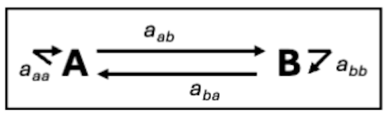
Consider a highly simplified case of two processes, both subject to selection, which may have mutually reinforcing or mutually limiting (competing) effects on each other, or where selection for one process supports or reinforces the other, which in turn limits it. Figure 2 shows the relationships between two components A, B which can be treated as a signed digraph by assigning positive or negative values to the axx links. We assume here that all links are nonzero, and that aaa, abb are both negative due to being subject to some limitations on their development. We consider first the case where aab and aba dominate the behavior (that is, neither component is near its limiting threshold).
If both links are negative, the system is dynamically unstable by the Routh-Hurwitz criteria [55] and a small perturbation will shift it to a new state. An example is the relationship between Earth’s ice cover and temperature. More ice cover increases albedo, reflecting more solar radiation and lowering temperatures (negative feedback). Temperature has a negative link to ice cover, as higher temperatures reduce ice and albedo. While these simple interactions are embedded within a vast network of climate feedbacks, they place a key role in transitions among global climate modes (e.g., [56,57]).
Mutual reinforcement occurs when aab, aba > 0. In this case increasing function or fitness of both components reinforces the other. One example is the relationship between erosion and weathering in geomorphological denudation. Weathering is a necessary precursor to erosion and provides transportable debris. Erosion promotes weathering via exposure of weatherable minerals. This configuration is also dynamically unstable, producing topographic dissection and other manifestations of divergent development as the reinforcing gradient and resistance selection processes push the landscape toward increasing spatial variability.
In some cases, aab > 0 and aba < 0 (or vice versa). These are dynamically stable, tending to maintain the system state except in the case of large changes and disturbances. The state of soil organic matter is the outcome of interactions between organic matter production (e.g., litterfall) and decomposition. Organic matter additions increase decay rates in most terrestrial environments, and higher decomposition rates in turn limit organic matter accumulation.
The three examples above all assume that aab, aba are stronger than the self-links. This assumption is violated when thresholds are approached and aaa or abb becomes dominant. In topographic evolution, for instance, depletion of weatherable minerals in weathering or incision to base level in erosion eventually limit divergent evolution, producing a mode shift to convergent development. In the soil organic matter example, if either vegetation production or decomposition becomes more limited (for instance by drought, temperature, or increased wetness), the dynamic steady-state is pushed to a new state.
These simplified binary dynamics can be generalized to larger-N cases, the key factor being whether there is net positive or negative feedback. Positive feedback and instability produces a positive largest Lyapunov exponent, indicating positive K-entropy, while net negative feedback and stability lead to the opposite. Therefore, ESS complexity as reflected in K-entropy may increase or decrease during evolution. Divergent, complexity-increasing evolution is common in ESS, but is generally inherently constrained by threshold limits. These commonly occur in the form of fundamental limits on key processes (e.g., maximum photosynthetic efficiency of plants or rates of chemical reactions), relative rates of linked processes (e.g., precipitation and evapotranspiration, uplift vs. denudation), storage capacities (e.g., sedimentary accommodation space, soil moisture storage capacity), and saturation-and-depletion phenomena, where resources have a positive or neutral effect up to some threshold, beyond which they have negative impacts (e.g., nutrients in ecosystems; moisture and redox reactions). Increases in complexity and diversity in ESS are therefore not open-ended. Similar suggestions have been made in a global context: Conway Morris [58] argued that biological systems are at or near their limits of complexity, and Hazen and Wong [20] speculated that Earth may be approaching the maximum limit of functional information for mineral genesis.
5. Discussion
Changes in complexity in evolving ESS are considered here in three ways—the complexity of the pattern of state changes represented by historical sequences and STMs, the number of different variations (richness) produced by evolution, and the number of actual or potential functional, fit, or adapted outcomes relative to the total possible.
5.1. Networks or Patterns of Evolutionary Change
Depending on how evolutionary sequences are understood or represented—and more importantly, on the nature of the sequences themselves—the pattern may range (in graph terms) from simple linear paths or convergence/divergence patterns to highly complicated networks of state transitions. In this context, complexity can only increase as the length or size of the sequence increases. However, both real and apparent changes in complexity may depend on whether evolution is considered step-by-step or as the starting point vs. the end point in a sequence of evolutionary state changes.
5.2. Richness and Variability
Evolutionary development can increase or decrease the richness of potential outcomes or the variability of ESS. The number of possible system states is a function of the available space and time for them to evolve and exist, “vergence”(the net effects of divergent and convergent development), the balance between creation or importation of new variants and loss of existing ones (IO), and canalization. Symbolically,
This is shown in discrete form due to the frequently episodic nature of changes, and the often-necessary study and representation of evolution in discrete terms, but an analog of eq. (19) in continuous form is possible.
Other things being equal (which is never the case in real ESS), the more space for different states to exist and the more time for states to develop, the more states there will be (time is incorporated in the Δt terms). This richness may be increased or decreased by the relative amounts of divergent and convergent evolution and will be decreased by canalization. S can be increased by influx of new variants from external sources, or the loss to extinction or outflux. Various combinations of the factors in eq. (19) occur in different Earth systems, at different spatial or temporal scales, and at different locations and times.
Earth systems are characterized by selection for multiple processes and components. The net negative and positive feedbacks lead to convergent or divergent evolution. Limiting thresholds keep either convergent or divergent modes from continuing indefinitely, resulting in mode switches, so that the same system may either increase or decrease in complexity during different periods of its evolution.
5.3. Functional Information
Viewed as a hierarchy of possibilities or microstates (section 3.2), constraining possibilities from the family of all quantum states to all laws applicable to ESS to evolution spaces, trajectory spaces, and finally to state transition spaces indicates an increase in functional information as different levels of selection come into play. That is because each additionally constrained level of selection reduces the possible functional solutions relative to the possibilities of the level above. Thus, functional information, as in the example of eq. (18), must increase.
However, within any but the top hierarchical level, the factors shown in eq. (19) and multiple simultaneous selection may result in increasing and/or decreasing complexity and functional information. Climate and other environmental changes may therefore result in greater or lesser complexity of landscapes, ecosystems, and other environmental systems. This in turn may have implications for the stability of ESS and for bio-, geo-, and pedodiversity. Stability is not always to be desired; for example, a hillside in the southeastern U.S. choked with the invasive kudzu vine (Pueria Montania) is very stable, but provides few ecosystem services. Instability can be problematic, of course, but in some ESS instability is necessary for adaptation, such as to droughts and sea-level rise [e.g., 4,10,25,28,43].
6. Conclusions
Is the universe becoming more complex? Perhaps. Are all constituents of the universe becoming more complex? No. Are Earth surface systems becoming more complex? Yes, no, and maybe.
Globally, biological and mineral evolution have increased their complexity, at least as indicated by functional information. However, there are suggestions that this is not open-ended and cannot continue indefinitely. More to the point of this study, functional information of ESS will increase if new possible states or configurations are spawned in greater numbers than the subset of states that are selected for some function (or if selection processes continue to prune less-fit options). Convergent evolution within a system and canalization can be viewed as reducing the functional options relative to what was previously possible, but they also reduce the future possibilities. Functional information may thus not inevitably increase, depending on the foreclosure rates of evolving functional states and potential future states—or on whether evolution is viewed as a step-by-step sequential process or as one or more starting states and a population of future possibilities.
Actual historical evolutionary sequences of state changes represent a linear path, regardless of other possible pathways and states. The embedded complexity of these sequences increases as they get longer. Similarly, historical sequences represented by other network structures can only get more complex as the graphs representing those networks are elaborated. These cases, however, deal with the complexity of the historical pattern of change, and do not bear on the richness or diversity of evolutionary outcomes. Other things being equal, the number of potential states is positively related to the amount of space and time for them to evolve, either of which may decrease as well as increase in ESS. Richness may also be increased by divergent evolution or decreased by convergent evolution and by canalization. The population of potential states may be increased by influx of new variants from external sources or reduced due to losses to extinction or outflux. Numerous combinations of these factors are found in different Earth systems, at different scales, and at different locations and times.
The ideas of function, fitness and adaptation and positive selection are complicated by the fact that ESS contain multiple components undergoing selection that may offset or reinforce each other. A simple model shows that such dynamics may produce dynamically stable, convergent, entropy-decreasing evolution that reduces variation within the system, or dynamically unstable, divergent, entropy-increasing evolution that increases variation. Numerous real-world examples of both phenomena (as well as steady states) exist.
Overall, it seems more fruitful to ask whether selection and evolution increase complexity in a specific system rather than to attempt to make statements about all systems.
Funding
This research received no external funding.
Data Availability Statement
All data used in this study are included in the text.
Acknowledgments
(to be added following review).
Conflicts of Interest
The author declares no conflicts of interest.
References
- Wolpert, D.H. Information width: A way for the second law to increase complexity. In Lineweaver, C.H., Davies, P.C.W., Ruse, M. (eds.) Complexity and the Arrow of Time, 2013. Cambridge University Press, p. 246-276.
- Lineweaver, C.H.; Davies, P.C.W.; Ruse, M. (eds.). Complexity and the Arrow of Time. Cambridge University Press, 2013, 357 p.
- Ball, P. Why everything in the universe turns more complex. Quanta Mag., 2025. https://www.quantamagazine.org/why-everything-in-the-universe-turns-more-complex 20250402/?mc_cid=a45a088c44, accessed 12 May 2025.
- Phillips, J.D. Landscape Evolution. Landforms, Ecosystems, and Soils. Elsevier, Amsterdam, 2021.
- Dennett, D.C. Darwin’s Dangerous Idea. Simon and Schuster, New York, 1995.
- Kaila, V.R.I.; Annila, A. Natural selection for least action. Proceedings of the Royal Society A 2008, 44, 3055–3070. [Google Scholar] [CrossRef]
- Sharma, V.; Annila, A. Natural process – Natural selection. Biophysical Chemistry 2007, 127, 123–128. [Google Scholar] [CrossRef] [PubMed]
- Nanson, G.C.; Huang, H.Q. Least action principle, equilibrium states, iterative adjustment and the stability of alluvial channels. Earth Surface Processes and Landforms 2008, 33, 923–942. [Google Scholar] [CrossRef]
- Phillips, J.D. Emergence and pseudo-equilibrium in geomorphology. Geomorphology 2011, 132, 319–326. [Google Scholar] [CrossRef]
- Phillips, J.D. Abiotic Selection in Earth Surface Systems. Geophysics and the Environment Series, Springer, 2025.
- Doménech, J.L.U.; Nescolarde-Selva, J.A.; Lloret-Climent, M. Structure, thermodynamics and information in complex systems. Kybernetes 2022, 52, 5307–5328. [Google Scholar] [CrossRef]
- Wong, M.L.; Cleland, C.E.; Arend, D., Jr.; et al. On the roles of function and selection in evolving systems. Proc. Natl. Acad. Sci. USA 2023, 102, e2320223120. [Google Scholar] [CrossRef]
- Phillips, J.D. Embedded complexity of evolutionary sequences. Entropy 2024, 26, 458. [Google Scholar] [CrossRef]
- Shannon, C.E. A mathematical theory of communication. Bell Syst. Tech. J. 1948, 27, 379–423, 623-656. [Google Scholar] [CrossRef]
- Dehmer, M.; Mowshowitz, A. A history of graph entropy measures. Inf. Sci. 2011, 181, 57–78. [Google Scholar] [CrossRef]
- Dehmer, M.; Mowshowitz, A. Generalized graph entropies. Complexity 2011, 17, 45–50. [Google Scholar] [CrossRef]
- Geller, W.; Kitchens, B.; Misiurewicz, M.; Rams, M. A spectral radius estimate and entropy of hypercubes. Int. J. Bifurc. Chaos 2012, 22, 1250096. [Google Scholar] [CrossRef]
- Mowshowitz, A.; Dehmer, M. Entropy and the complexity of graphs revisited. Entropy 2012, 14, 559–570. [Google Scholar] [CrossRef]
- Szostak, J.W. Molecular messages. Nature 2003, 423, 689. [Google Scholar] [CrossRef]
- Hazen, R.M.; Wong, M.L. Open-ended versus bounded evolution: Mineral evolution as a case study. PNAS Nexus 2024, 3, 248. [Google Scholar] [CrossRef]
- Kapitaniak, T. 1988. Chaos in Systems with Noise. Singapore: World Scientific.
- Culling, W.E.H. Dimension and entropy in the soil-covered landscape. Earth Surf. Process. Landf. 1988, 13, 619–648. [Google Scholar] [CrossRef]
- Rankey, E.C. 2003. Carbonate coasts as complex systems: A case study from Andros Island, Bahamas. Coastal Sediments 2003. American Society of Civil Engineers, New York, pp. 1–9.
- Phillips, J.D. Signatures of divergence and self-organization in soils and weathering profiles. J. Geol. 2000, 108, 91–102. [Google Scholar] [CrossRef]
- Ibanez, J.J. Evolution of fluvial dissection landscapes in Mediterranean environments: Quantitative estimates and geomorphic, pedologic, and phytocenotic repercussions. Z. Geomorph. 1994, 38, 105–119. [Google Scholar]
- Phillips, J.D.; Gares, P.A.; Slattery, M.C. Agricultural soil redistribution and landscape complexity. Landscape Ecol. 1999, 14, 197–211. [Google Scholar] [CrossRef]
- Toomanian, N.; Jalalian, A.; Khamedi, H.; Eghbal, M.K.; Papritz, A. Pedodiversity and pedogenesis in Zayandeh-red Valley, central Iran. Geomorphology 2006, 81, 376–393. [Google Scholar] [CrossRef]
- Phillips, J.D.; Walls, M.D. Flow partitioning and unstable divergence in fluviokarst evolution in central Kentucky. Nonlinear Processes in Geophysics 2004, 11, 371–381. [Google Scholar] [CrossRef]
- Dehmer, M.; Emmert-Streib, F.; Shi, Y. Interrelations of graph distance measures based on topological indices. PLoS ONE 2014, 9, e94985. [Google Scholar] [CrossRef] [PubMed]
- Briske, D.D.; Fulendor, S.D.; Smeins, F.E. State-and-transition models, thresholds, and rangeland health: A synthesis of ecological concepts and perspectives. Range. Ecol. Manag. 2005, 58, 1–10. [Google Scholar] [CrossRef]
- Bestelmeyer, B.T.; Tugel, A.J.; Peacock, D.G.; Robinett, D.G.; Shaver, P.L.; Brown, J.R.; Herrick, J.E.; Sanchez, H.; Havstad, K.M. State-and-transition models for heterogeneous landscapes: A strategy for development and application. Range. Ecol. Manag. 2009, 62, 1–15. [Google Scholar] [CrossRef]
- Phillips, J.D.; Van Dyke, C. Geomorphological state-and-transition models. Catena 2017, 153, 168–181. [Google Scholar] [CrossRef]
- Phillips, J.D. Laws, place, history and the interpretation of landforms. Earth Surface Processes & Landforms 2017, 42, 347–354. [Google Scholar] [CrossRef]
- Simpson, G.G. 1963. Historical science. In: Albritton, C.C. (Ed.), The Fabric of Geology. Freeman, Cooper & Co., Stanford, CA, pp. 24–48.
- Retallack, G.J. 2001. Soils of the Past. An Introduction to Palaeopedology, 2nd ed. Blackwell, Chichester, UK.
- Krivovichev, S.V.; Krivovichev, V.G.; Hazen, R.M. Structural and chemical complexity of minerals: Correlations and time evolution. Eur. J. Mineral. 2018, 30, 231–236. [Google Scholar] [CrossRef]
- Hazen, R.M.; Downs, R.T.; Eleish, A.; et al. Data-driven discovery in mineralogy: Recent advances in data resources, analysis, and visualization. Engineering 2019, 5, 397–405. [Google Scholar] [CrossRef]
- Lineweaver, C.H. A simple treatment of complexity: Cosmological entropic boundary conditions on increasing complexity. In Lineweaver, C.H., Davies, P.C.W., Ruse, M. (eds.) Complexity and the Arrow of Time, 2013. Cambridge University Press, p. 42-67.
- Nanson, G.C.; Huang, H.Q. Self-adjustment in rivers: Evidence for least action as the primary control of alluvial-channel form and process. Earth Surface Processes and Landforms 2017, 42, 575–594. [Google Scholar] [CrossRef]
- Nanson, G.C.; Huang, H.Q. A philosophy of rivers: Equilibrium states, channel evolution, teleomatic change and the least action principle. Geomorphology 2018, 302, 3–19. [Google Scholar] [CrossRef]
- Phillips, J.D. Evolutionary creativity in landscapes. Earth Surface Processes and Landforms 2020, 45, 109–120. [Google Scholar] [CrossRef]
- Hunt, A.G.; Faybishenko, B.; Ghanbarian, B. Non-linear hydrologic organization. Nonlinear Processes in Geophysics 2021, 28, 599–614. [Google Scholar] [CrossRef]
- Phillips, J.D. Contingent partitioning and adaptation in hydrological systems. Ecohydrology 2023, 16, e2567. [Google Scholar] [CrossRef]
- Wang, Q.; Zhang, Y.; Cheng, Z.; et al. Formation mechanisms of Qiaoba-Zhongdu Danxia landforms in southwestern Sichuan Province, China. Open Geosciences 2024, 16, 20220709. [Google Scholar] [CrossRef]
- Waddington, C.H. Canalization of development and the inheritance of acquired characteristics. Nature 1942, 150, 563–565. [Google Scholar] [CrossRef]
- Caloi, P. On the canalization of seismic energy. Ann. Geophys. 1964, 17, 513–522. [Google Scholar]
- Berlow, E.L. From canalization to contingency: Historical effects in a successional rocky intertidal community. Ecol. Monogr. 1997, 67, 435–460. [Google Scholar] [CrossRef]
- Levchenko, V.F.; Starobogatov, Y.I. Evolution of life as improvement of management by energy flows. Int. J. Comp. Anticipat. Syst. 1999, 5, 199–220. [Google Scholar]
- Stallins, J.A. Geomorphology and ecology: Unifying themes for complex systems in biogeomorphology. Geomorphology 2006, 77, 207–216. [Google Scholar] [CrossRef]
- Naylor, L.A.; Stephenson, W.J. On the role of discontinuities in mediating shore platform erosion. Geomorphology 2010, 114, 89–100. [Google Scholar] [CrossRef]
- Verleysdonk, S.; Krautblatter, M.; Dikau, R. Sensitivity and path dependence of mountain permafrost systems. Geogr. Ann. Phys. Geogr. 2011, 93, 113–135. [Google Scholar] [CrossRef]
- Wainwright, J.; Turnbull, L.; Ibrahim, T.G.; Lexartza-Artza, I.; Thornton, S.F.; Brazier, R.E. Linking environmental regimes, space and time: Interpretations of structural and functional connectivity. Geomorphology 2011, 126, 387–404. [Google Scholar] [CrossRef]
- Perron, T.; Fagherrazi, S. The legacy of initial conditions in landscape evolution. Earth Surf. Process. Landforms 2012, 37, 52–63. [Google Scholar] [CrossRef]
- Phillips, J.D. Complexity of Earth surface system evolutionary pathways. Mathematical Geosciences 2016, 48, 743–765. [Google Scholar] [CrossRef]
- Cesari, L. Asymptotic Behavior and Stability Problems in Ordinary Differential Equations. Springer, New York, 1971.
- Pedro, J.B.; Jochum, M.; Buizert, C.; et al. Beyond the bipolar seesaw: Toward a process understanding of interhemispheric cooling. Quat. Sci. Rev. 2018, 192, 27–46. [Google Scholar] [CrossRef]
- Wunderling, N.; von der Heydt, A.S.; Akseny, Y.; et al. Climate tipping point interactions and cascades: A review. Earth Syst. Dyn. 2024, 15, 41–74. [Google Scholar] [CrossRef]
- Conway Morris, S. Life: The final frontier for complexity? In Lineweaver, C.H., Davies, P.C.W., Ruse, M. (eds.) Complexity and the Arrow of Time. 2013. Cambridge University Press, p. 135-161.
Figure 1.
Summary of the hierarchy of possible landscape states and transitions. N = number of potential states, m = number of possible transitions among states; n( ) indicates cardinality.
Figure 1.
Summary of the hierarchy of possible landscape states and transitions. N = number of potential states, m = number of possible transitions among states; n( ) indicates cardinality.
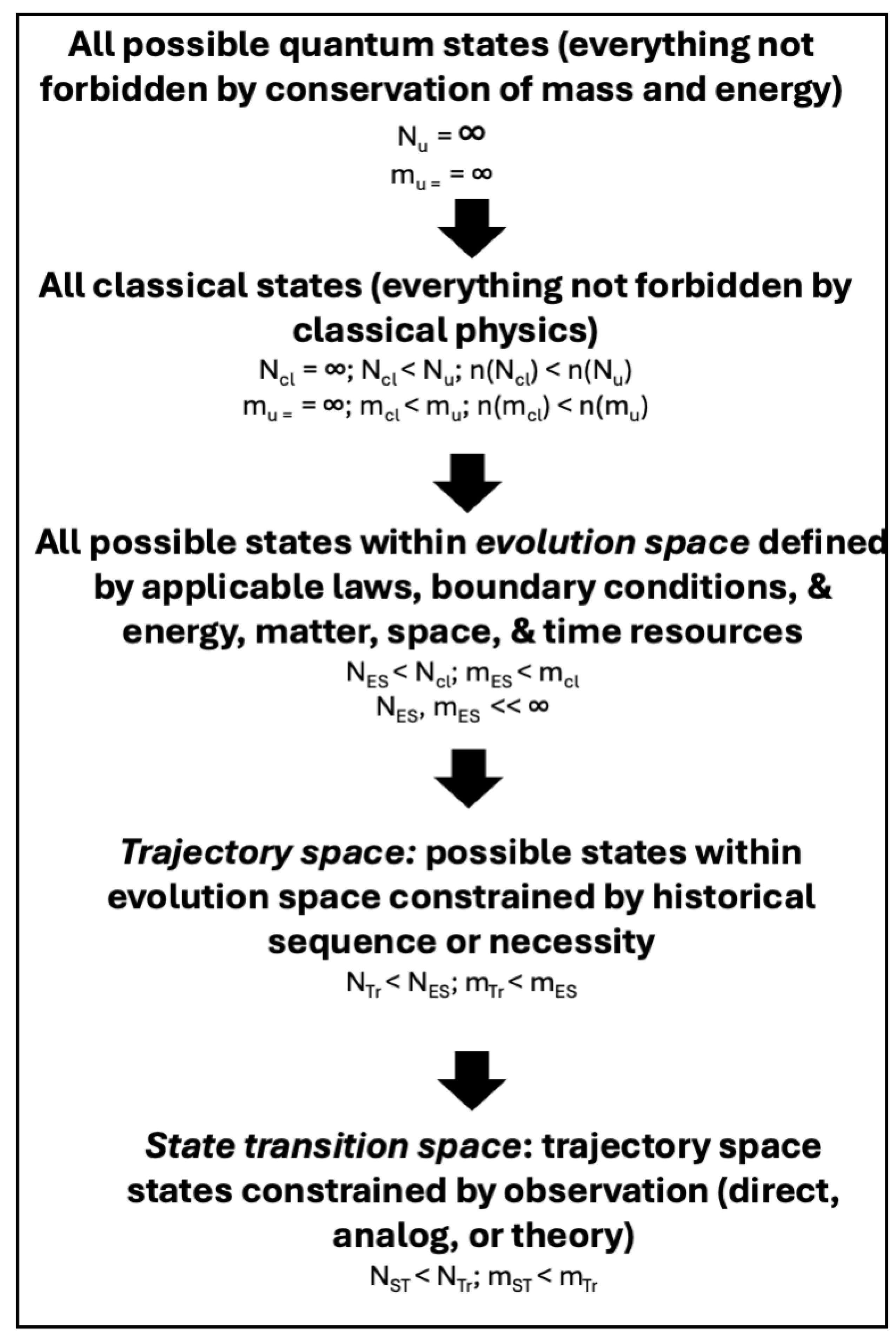
Figure 2.
Feedbacks in a simplified two-component ESS.
Disclaimer/Publisher’s Note: The statements, opinions and data contained in all publications are solely those of the individual author(s) and contributor(s) and not of MDPI and/or the editor(s). MDPI and/or the editor(s) disclaim responsibility for any injury to people or property resulting from any ideas, methods, instructions or products referred to in the content. |
© 2025 by the authors. Licensee MDPI, Basel, Switzerland. This article is an open access article distributed under the terms and conditions of the Creative Commons Attribution (CC BY) license (http://creativecommons.org/licenses/by/4.0/).
Copyright: This open access article is published under a Creative Commons CC BY 4.0 license, which permit the free download, distribution, and reuse, provided that the author and preprint are cited in any reuse.


