
Submitted:
22 May 2025
Posted:
23 May 2025
You are already at the latest version
Abstract
In this study, we aim to control several customer characteristics by leveraging the properties of upstream manufacturing processes. We introduce an innovative approach that marries an enhanced Partial Least Squares (PLS) regression technique, tailored to output vectors, with Hotelling's T2 control chart. The fusion of these methods allows for the simultaneous control and regulation of all upstream factors influencing multiple outcomes, distilled into a single control chart for streamlined monitoring. Our method advances the current frontier of predictive Statistical Process Control (SPC), facilitating a multi-objective governance of manufacturing operations. This strategy notably simplifies the task of concurrently tracking numerous end-user attributes and their corresponding upstream factors. Empirical evidence underlines the prowess of our methodology in predicting client-specific features and in flagging early signals of perturbations in upstream process stability.
Keywords:
multi‐objective
; statistical process control
; multivariate
; partial least squares
1. Introduction
Despite the plethora of Statistical Process Control (SPC) techniques documented in scholarly work, they essentially bifurcate into two principal categories: univariate and multivariate, as delineated by Sanchez-Marquez & Jabaloyes Vivas (2020). Both paradigms, however, are grounded in a shared foundational concept: the imperative to govern upstream factors or variables. By controlling the relevant or critical upstream variables, one can secure the consistency and predictability of the downstream variables they affect.
The traditional approach of utilising univariate SPC methods to manage manufacturing processes involves plotting each critical upstream variable individually on its chart, as outlined by Aunali and Venkatesan (2019). Techniques such as the product tree, process mapping, or quality function deployment (QFD) have been established to identify these upstream characteristics (Chan & Wu, 2002). Nevertheless, Sanchez-Marquez and Jabaloyes Vivas (2020) have highlighted a significant drawback of this approach: its ineffectiveness in anticipating the behaviour of downstream characteristics. Consequently, such univariate methods may overlook or misjudge potential deviations in the final product attributes, which are vital in satisfying customer expectations (Sanchez-Marquez et al., 2020). Section 2 and Section 3 of this paper corroborate the findings of Sanchez-Marquez and Jabaloyes Vivas (2020), reinforcing the limited capacity of univariate charts to predict deviations in downstream characteristics. Moreover, the complexity associated with managing many upstream variables—often requiring one or two charts per variable—can lead to an overwhelming number of charts, thus making univariate SPC approaches inefficient and impractical.
In contrast, multivariate SPC methods, such as Hotelling’s T2 statistic (Hotelling, 1947), calculate a single value that captures the square deviation of each measurement from the mean vector. By relying on only one statistic, the multivariate T2 chart proves to be more effective than univariate methods, which often require multiple control charts to monitor multiple statistics. Multivariate charts can detect deviations across any variable consolidated within them. After Hotelling’s work, researchers have adapted multivariate methods for distinct industries (Ferrer, 2007; Mehmood et al., 2022; Borràs-Ferrís et al., 2025), employing multivariate statistics founded on the dimensional reduction techniques of principal component analysis (PCA) or PLS models. However, these methods do not use PLS as a regression tool, which means they need to consider the regression coefficients, and thus, the influence of predictors is neglected. As Sanchez-Marquez and Jabaloyes Vivas (2020) indicated, this can lead to a tendency to signal an excess of deviations, given that all upstream variables are treated with equal significance. Section 2 of this paper also supports this notion by presenting results that align with these observations.
Furthermore, the PLS algorithm has been the foundation for multivariate methods that address time-domain variables, where predictor measurements are captured by segmenting variables across time (Macgregor et al., 1994; Figueiredo et al., 2016; Zhao & Huang, 2022; Jorry et al., 2025). This practice is common in industries like the chemical sector, where continuous processes prevail. In these scenarios, researchers have endeavoured to mitigate the effects of autocorrelation when employing time-series data (James et al., 2013; Wang et al., 2021). Nonetheless, within the manufacturing context—this paper’s focus—measurements are derived from distinct units rather than temporal discretisation and are thus considered independent observations without autocorrelation issues (Ferrer, 2007; Sanchez-Marquez & Jabaloyes Vivas, 2020; Borràs-Ferrís et al., 2025).
In the era of big data and the advent of Industry 4.0, the relevance of multivariate Statistical Process Control (SPC) methods has surged. However, a persistent challenge with these methods is interpreting signals when a process deviates from its expected behaviour (Bersimis et al., 2009). Upon the emergence of an out-of-control signal, it is incumbent upon practitioners to diagnose the upstream factors responsible for the downstream deviation to fix the issue and prevent its recurrence. Furthermore, Sanchez-Marquez and Jabaloyes Vivas (2020) advocate for incorporating regression coefficients to bolster the predictability of downstream characteristics.
In manufacturing, where observations are intrinsically independent, adherence to the assumptions concerning residuals is imperative for the integrity of a predictive model (Walpole et al., 1993). The merit of a model is substantiated by scrutinising regression residuals and the coefficient of determination (a robust R2 value). Notably, nonlinear relationships between output and input variables may be captured using higher-order polynomials and alternative transformations, such as step functions or splines. Under such circumstances, the assumption of linearity can be confined to the regression coefficients alone (James et al., 2013). Nonetheless, maintaining an equilibrium between predictability and the clarity of signal interpretation is crucial within this work, as practitioners must be equipped to discern and adjust upstream factors that cause unstable signals.
A significant drawback of nonparametric methods lies in the necessity for explicit mathematical models that practitioners can employ to trace the root cause of signals indicating control process deviations (Sanchez-Marquez & Jabaloyes Vivas, 2020; Sanchez-Marquez et al., 2020). For instance, Support Vector Regression (SVR) models express curvature by applying kernel functions—sophisticated mathematical constructs that can prove challenging to interpret. However, it is equally feasible to model curvature through kernel transformations (Aggarwal, 2015). Moreover, in manufacturing and continuous improvement, sample sizes are frequently limited. Research by James et al. (2013) demonstrates that parametric methods have a superior performance over nonparametric ones in small-sample contexts. This evidence underpins the selection of PLS as the method of choice for multivariate SPC methods that utilise predictive models, as elucidated by Sanchez-Marquez and Jabaloyes Vivas (2020).
Moreover, when using PLS regression models instead of latent variable-based methods, the assumptions regarding the normal distribution of predictors are mitigated (Sanchez-Marquez & Jabaloyes Vivas, 2020). While multivariate statistics typically operate effectively with a relaxed assumption of a multivariate normal distribution—contingent on the absence of outliers and a symmetrical distribution (Peña, 2002; Rencher, 2005)—the fundamental tenets of linear regression (independence, normality, and equal variance) are relevant to the residuals, except for linearity which pertains to the input-output relationship (Walpole et al., 1993; James et al., 2013).
PLS has been chosen for its congruence with the aims of this investigation, as corroborated by the rationale above, which is based on the following features (see above for details and related references):
- -
- It is well-known that PLS has an explicit regression model that eases interpretation and the ulterior fixing of causes of instability.
- -
- PLS has proved to be efficient in manufacturing environments affected by high complexity.
- -
- PLS is a parametric method that is thus efficient for small sample sizes, even with more predictors than observations, which are typical in manufacturing. This characteristic is unique to the PLS algorithm.
- -
- Although the PLS algorithm is based on the normal assumption of the predictors, it can be relaxed when using PLS as a regression model instead of the latent variables to construct the multivariate chart.
- -
- PLS can model nonlinear relationships between output and input variables, so linearity is referred only to the regression coefficients.
In their seminal work, Sanchez-Marquez and Jabaloyes Vivas (2020) developed an advanced multivariate partial least squares (PLS) regression methodology tailored to predict downstream variables and construct the corresponding SPC charts. This technique represents a significant leap over traditional univariate and multivariate SPC methods, offering enhanced predictability, superior early warning capabilities, and a streamlined approach to complexity management.
Nevertheless, industry 4.0 has ushered in an era marked by intricate interactions between upstream and downstream factors (input and output variables). Many upstream predictors frequently govern several interrelated outputs in this environment, weaving a web of complex relationships, as Palací-López et al. (2020) noted. These connections among numerous predictors and an output vector are typically modelled by a matrix equation y = Bx, where ’y’ denotes the output vector, ’x’ is the input vector, and ’B’ is the coefficient matrix. This configuration is often called a coupled/decoupled design, a term coined by Suh (2005). In this complex context, Sanchez-Marquez and Jabaloyes Vivas (2020) utilised multivariate regression techniques to construct individual SPC charts for each downstream characteristic. This approach simplifies the complexity inherent in univariate methods, offering a more cohesive framework for monitoring and control in modern manufacturing environments.
Building on the enhancements to traditional univariate and multivariate methods by Sanchez-Marquez and Jabaloyes Vivas (2020) regarding predictability and early detection, this paper proposes a further refinement to streamline these approaches. The key innovation lies in integrating regression models with multivariate SPC charts, thus enabling the prediction and control of multiple interrelated downstream variables through a single multivariate chart. The essence of this paper is to present a methodology that evolves the work of Sanchez-Marquez and Jabaloyes Vivas (2020) by reducing its complexity without compromising its fundamental strengths.
The methodology introduced in this paper exploits an attribute of PLS regression (Geladi and Kowalski, 1986a, 1986b; Lin et al., 2023) for predicting several output characteristics (yj). Additionally, it proposes the construction of a single multivariate SPC chart that encapsulates all these predictions, thereby diminishing the complexity associated with individually monitoring each variable. This approach has the strengths of both approaches, addressing the challenges of over-detection in traditional multivariate SPC methods and the complexities inherent in univariate SPC techniques, as identified by Sanchez-Marquez and Jabaloyes Vivas (2020).
The proposed methodology employs a multivariate control chart to consolidate all predicted downstream variables, necessitating an estimation of the covariance matrix to align with the no-outlier assumption and enhance detection sensitivity. This essential estimation process for the in-control covariance matrix, crucial for computing Hotelling’s T2 statistic, is referenced in existing literature (Ferrer, 2007; Zhao & Huang, 2022; Jorry et al., 2025) but will be detailed in the upcoming section due to its significance in ensuring method sensitivity. The estimation procedure shares a theoretical foundation with established methods but is tailored to function with predictive models. Given its direct bearing on the fundamental assumptions of the statistic employed, it is a critical factor that could affect the control chart’s capacity to identify out-of-control signals. The forthcoming sections, alongside a Matlab script provided as supplementary material (Sanchez-Marquez, 2023), will furnish comprehensive details on adhering to these assumptions.
The following sections detail a method that innovatively utilises the PLS regression algorithm to amplify its predictive capacity for vector outputs. This novel application draws upon a characteristic of the PLS algorithm initially identified by Geladi & Kowalski (1986a, b), which typically confers an advantage to PLS over principal component regression (PCR). Unlike PCR, where latent variables are determined separately from the input and output data and subsequently correlated through ordinary least squares (OLS) regression, PLS extracts latent variables concurrently from both the input and output data matrices. This concurrent extraction induces a rotation in the latent variables relative to those derived from PCR, facilitating an enhanced explanation of the input-output relationship, thus increasing the model’s R2. By taking advantage of the rotatability of the latent variables, the PLS algorithm allows the regression coefficients to better fit the output data used in the regression model. This paper aims to fully exploit this distinctive aspect of the PLS algorithm to maximise the predictive power of regression models derived from the data. Appendix A details how the PLS algorithm extracts the latent variables used to build the regression model.
In essence, the method delineated in this paper extends the technique of Sanchez-Marquez and Jabaloyes Vivas (2020) for scenarios wherein the output is a vector rather than an isolated variable. This method aims to predict an array of downstream characteristics linked to an SPC chart, deriving its predictive models from upstream factors. This innovative strategy enhances the general application of the PLS algorithm by maximising the predictive efficacy of the multivariate regression model, as measured by the coefficient of determination R2.
Therefore, the objectives of this paper can be expressed by two main research questions:
1. Can we summarise various downstream characteristics within a multivariate chart while preserving the sensitivity to detect anomalies caused by upstream variables?
2. Can PLS regression be refined to enhance its predictive accuracy for vector outputs, which represent multiple downstream characteristics concurrently?
Addressing the above questions is the objective of this paper since they anchor on the axiom that multivariate SPC methods grounded in predictive models are more effective when these models exhibit a high coefficient of determination (R2), as argued by Sanchez-Marquez & Jabaloyes Vivas (2020) and Sanchez-Marquez et al. (2020).
This paper validates the method through its application in a case study. Accompanying this paper is a complete Matlab script provided as supplementary data, which incorporates a new and refined PLS approach (Sanchez-Marquez, 2023). This approach increases the predictive capabilities of PLS models, making them suitable for vector outputs or multi-objective problems that involve multiple related downstream characteristics. A methodology for interpreting instability signals and identifying upstream determinants has also been formulated.
The findings affirm the anticipated outcome: the advanced PLS algorithm conceived in this research amplifies the predictive prowess of the multi-objective multivariate SPC method (multi-objective MSPC-PLS). This refinement has facilitated the detection of out-of-control signals by monitoring dozens of predictors via a unified multivariate chart.
The next sections are structured as follows:
Section 2. Proposed method and case study results. This section develops the proposed method based on theoretical foundations while showing its validity using data from a manufacturing case study. It analyses the case study results in the context of the objectives detailed by the research questions written above.
Section 3. Discussion. This section further analyses the results regarding theoretical contributions, practical implications, and research limitations.
Section 4. Conclusions. This section outlines the main conclusions of the research.
Appendix A. PLS algorithm. In this appendix, the PLS algorithm is detailed to understand the mathematical foundations of this paper. Since the PLS method is based on an algorithm and not on a simple mathematical model, a separate appendix enhances the flow and readability of the paper.
2. Materials and Methods
This section develops the foundational principles of the proposed method through a structured multistep sequence, augmented by a case study, to demonstrate its practical application and to assess its validity and effectiveness.
To be aligned with customer expectations, final customer characteristics (yj) must be regulated, typically by reducing variability. Sanchez-Marquez and Jabaloyes Vivas (2020) elucidated the process of employing empirical predictive models based on upstream variables (xi) to construct multivariate SPC charts, highlighting the benefits of this strategy over conventional univariate and multivariate SPC methods. However, the approach delineated permits the creation of only a single chart for each customer characteristic. As noted in the introductory section, the contemporary environment of Industry 4.0 and the proliferation of big data necessitates tackling intricate issues where many predictors influence several (that can be even correlated) downstream characteristics, resulting in either coupled or decoupled designs (Suh, 2005). Sanchez-Marquez and Jabaloyes Vivas (2020) postulated that PLS regression is the preferred parametric technique for deriving the predictive models required to apply continuous improvement methodologies systematically. They also acknowledged that Multiple Linear Regression (MLR) could be a viable alternative, owing to its simplicity and effectiveness, which are on par with PLS. Nonetheless, the method exposed herein employs PLS due to its enhanced predictive capabilities when confronted with complex issues (Sanchez-Marquez & Jabaloyes Vivas, 2020) and other reasons presented in the preceding section. Given that the aim is to monitor several customer-related characteristics through a single chart, employing identical predictors (coupled/decoupled design), the predictive strength of the regression models becomes crucial for the control chart’s capacity to discern out-of-control signals.
The present method innovatively utilises the PLS algorithm to fully leverage its predictive potential, as Geladi and Kowalski (1986a) articulated, thereby maximising the efficacy of these regression models. While not displayed herein, nonlinear models employing higher-order polynomials were also explored (refer to the introductory section) to enhance the predictive accuracy of the regression models. Nevertheless, the coefficient of determination (R2) did not manifest any marked enhancement in this case study, leading to the inference that the relationship between output variables and predictors is linear.
As previously stated, this method is tailored for complex scenarios, which can be represented by Equation (1):
where y is the vector of the p outputs (downstream variables or customer characteristics), B is a p x m matrix that contains the regression coefficients (aka design matrix or coefficients matrix), and x is the vector that contains the m inputs (predictors or upstream variables).
y = Bx,
In line with the framework postulated by Suh (2005), design matrices can be categorised into three distinct types. The forthcoming exemplifications explain this classification within the scope of a scenario encompassing three outputs and inputs. However, the principles are extensible to a broader range of input and output variables. The tripartite classification of the design matrix is described as follows:
- A diagonal design matrix characterises an uncoupled design. Within such a design paradigm, the calibration of each output variable via its corresponding input variables (referenced in Equation (1)) is executed in isolation from the other output variables.
- 2.
- A triangular design matrix signifies a decoupled design. This configuration facilitates the independent adjustment of each output variable, provided that the adjustments are made in a prescribed sequence (Suh, 2005).
- 3.
- A coupled design represents the general case and is distinguished by a non-diagonal and non-triangular design matrix. In such a framework, the calibration of each output variable is interdependent, as alterations to one output variable have repercussions on the other output variables.
The methodology introduced herein is particularly efficient for scenarios typified by decoupled and coupled designs, where multivariate approaches have a pronounced advantage over conventional univariate techniques. These scenarios often involve multicollinearity among predictors—an aspect where multivariate PLS regression exhibits its strength (Rodriguez-Rodriguez et al., 2009; Sanchez-Marquez & Jabaloyes Vivas, 2020; Borràs-Ferrís et al., 2025)—and correlated outputs, which are beneficially addressed by the multivariate Hotelling’s T2 control chart (Ferrer, 2007). The efficacy of the method across these contexts is subsequently demonstrated. Nevertheless, the method retains its applicability across all three design types detailed above, with multivariate SPC methods offering a significant reduction in complexity relative to traditional univariate methods.
The following subsections articulate the method in steps, outlining the sequence practitioners should follow for its implementation. Theoretical foundations are provided, and empirical results from each stage of the method’s application are presented within the context of a case study in the automotive industry. The complete original Matlab script employed for the case study and the raw data about the measured upstream and downstream variables are available as supplementary materials accompanying this article (Sanchez-Marquez, 2023).
STEP 1. Model discovery.
The principal aim of this phase is to derive the influence of upstream variables (predictors) on downstream variables (customer characteristics). It will be accomplished by constructing a multivariate empirical model utilising PLS regression in alignment with the previously established rationale. Following the formulation of regression models for each downstream variable, the predicted values are synthesised and observed via a multivariate control chart, thereby streamlining the complexity of monitoring.
Within the paradigm of continuous improvement, work teams identify opportunities for enhancement (improvement projects) based on their potential impact on customer satisfaction. Such improvement projects frequently exert simultaneous influence on multiple customer characteristics. A consistent set of predictors can govern these characteristics, hence giving rise to complex interrelations (Palací-Lopez et al., 2020) as delineated earlier (refer to Equation (1)). Within this context, an essential tactic involves stabilising customer characteristics by controlling upstream characteristics (Sanchez-Marquez & Jabaloyes Vivas, 2020). After identifying the pertinent group of upstream variables, the initial step entails deriving the empirical model that delineates the relationship between upstream and downstream variables.
Geladi and Kowalski (1986a, b) provide an in-depth exposition of the workings of the PLS algorithm. This algorithm derives latent variables (represented by matrices T and U) as projections from the input matrix (X) and the output matrix (Y). As they demonstrated, these latent variables are oriented towards the same orientation that Principal Component Regression (PCR) would yield. PCR computes latent variables independently using the input and output matrices. These latent variables are subsequently employed to calculate the regression coefficients via Ordinary Least Squares (OLS).
In contrast, PLS procures latent variables through a reciprocal exchange of information between X and Y (refer to Appendix A for a comprehensive explanation). The iterative nature of this exchange process between input and output matrices ensures that the resultant latent variables encapsulate both data blocks more effectively than those derived from PCR (Geladi & Kowalski, 1986a; b). The PLS algorithm modulates the orientation of the latent variables—and thereby the regression coefficients—in response to the input and output matrix information, aiming to maximise the explained variance of these variables. PLS is versatile, accommodating scenarios involving a single output variable and multiple output variables, thus forming an output vector (Geladi & Kowalski, 1986a). In instances involving multiple outputs, the regression equation is formulated simultaneously as a matrix equation, expressed as
where Y denotes the n x p matrix encapsulating n multivariate observations across p output variables (customer characteristics), while X represents the n x m matrix containing n multivariate observations of m input variables (predictors). The matrix B, sized m x p, comprises the regression coefficients correlating m input variables with p output variables, also referred to as the design matrix or coefficient matrix. Equation (2) can be derived through regression by employing the complete output matrix Y or by deriving separate regression equations for each output variable before joining them to form Equation (2). In the latter approach, where regression coefficients are determined individually, the latent variables from which these coefficients are deduced will be oriented to reflect each output variable more accurately. Consequently, if the coefficients are estimated independently, they will provide a more precise prediction of the output variables, and the coefficient of determination (R2) for each output variable will be optimised. While deriving each regression equation one by one may appear less streamlined, the optimisation of R2 is vital for the proficiency of multivariate SPC methods based on predictive models (Sanchez-Marquez & Jabaloyes Vivas, 2020). Hence, diverging from the conventional application of PLS that constructs Equation (2) in its entirety at once, the method presented in this document employs the regression equation pertinent to each output variable discretely. Subsequently, each column of Y corresponds to one of the p vectors yi, originating from each of the p regression equations, which are structured as follows:
where yi is the ith output vector that contains the n univariate observations for the ith output variable. X is the input n x m matrix (the same as in Eq. (2)), and bi is the column vector that contains the m regression coefficients for the ith output variable. Therefore, in this method, for p output variables, Eq. (2) will be built as follows:
Y = XB,
yi = Xbi,
Appendix A details how the PLS algorithm extracts latent variables from the input and output data matrices to obtain Eq.’s regression coefficient matrix—matrix B (2).
During the case study, the project team identified four output variables essential to explain the geometric positioning of a component within the final product (p = 4). Given that the precise geometric alignment of this element was critical to customer satisfaction, its consistent stability was deemed a priority. The quartet of variables was integral to defining the part’s geometric stance. In a collaborative brainstorming session, the team selected 34 potential predictor variables (m = 34).
An orchestrated exercise was conducted to secure measurements for the 34 predictors and the four output variables from the maximum number of units feasible. Upon excluding observations (rows) with missing or erroneous data, the resultant dataset comprised measurements from 55 units (spanning 55 rows; n = 55) across the 38 variables (encompassing 38 columns; m + p = 38). In contemporary settings, it is assumed that processes are automated to facilitate the measurement and archival of such data. Nevertheless, not all processes are inherently designed with the requisite traceability to accurately acquire the measurements needed to implement the SPC method predicated on predictive models. This traceability is fundamental to constructing the database necessary for the application of this method, as it requires all measurements to be catalogued in association with a specific unit and variable. Sánchez-Márquez and Jabaloyes Vivas (2020) delve further into this topic, offering a more comprehensive discussion.
Table 1 and Table 2 show the predictive prowess of models derived using the same data but different methods. Therefore, they use the same sample size, so both tables are comparable to assess which method is more efficient in predictability. If practitioners needed a more general rule on what minimum sample size to derive a precise model, it could be established n = 32 since it is well-known that, in linear models, the R2 is the autocorrelation coefficient to the square (R2 = ρ2) and the point estimate of ρ (and thus the one of the R2) is a t statistic with n-2 degrees of freedom. It is also well-established that the t-statistic shows an asymptotic behaviour from 30 degrees of freedom, so n=32.
Table 1 shows the R2 of the four output variables obtained with PLS by regressing the four output variables at once on X (traditional approach).
Sanchez-Marquez et al. (2020) indicate that among the four models in Table 1, only the model corresponding to y3 can be ascribed to very strong predictive strength. Another model is deemed to have moderate predictive capacity, while the remaining models possess strong predictive power. In concordance with the guidance provided by Sanchez-Marquez and Jabaloyes Vivas (2020), enhancing the predictive power of these models is imperative. Leveraging the capabilities of the PLS function delineated above (also detailed in Appendix A), four distinct models were developed using PLS by individually regressing each output variable against X. The coefficient of determination (R2) values derived from this method are presented in Table 2.
As anticipated, the predictive prowess of the four models—which estimate the values of the four output variables—experienced an increase, as evidenced in Table 2. In the context of this case study, the enhancement in model performance is notably substantial, with each model now qualifying as at least ’strong’ in terms of predictive capability. Specifically, the models corresponding to y1 and y3 have attained a level of predictive power classified as ’very strong,’ while the models for y2 and y4 are now supported by ’strong’ predictive power. The complete Matlab scripts reflecting both methodologies are provided as supplementary materials in conjunction with this paper (Sanchez-Marquez, 2023).
It merits mention that the version of the PLS algorithm employed in this method—and consequently in this case study—is the refined iteration introduced by Sanchez-Marquez and Jabaloyes Vivas (2020). This advanced variant enhances model precision by excluding predictors whose coefficients are an order of magnitude smaller than the others, either by setting their coefficient value to zero or omitting them entirely. This refinement diminishes the noise within the predicted output, thus elevating the coefficient of determination (R2) and amplifying the model’s predictive power.
STEP 2. Build the complete model Y=XB using the y=Xb models
The previous phase has demonstrated that predictive power is maximised by independently deriving models for each output variable. At this juncture, it is imperative to compile the comprehensive matrix Y. Equation (4) illustrates the procedure for constructing the entire model in matrix form, denoted as Y=XB, by adjoining the individual models represented by y=Xb.
Due to spatial constraints, it is impracticable to replicate the complete model, which encompasses 34 predictors and four output variables, within the confines of this text. However, this objective is fulfilled by the Matlab script accompanying this paper, enabling a thorough examination of the model’s construction (Sanchez-Marquez, 2023).
STEP 3. Multivariate T2 chart for Y and model validation.
This step aims to build the multivariate Hotelling’s T2 control chart for Y and validate that the multivariate model has sufficient sensitivity to detect out-of-control signals. Therefore, to ensure enough sensitivity, it is necessary to calculate Hotelling’s T2 statistic for all observations (for the real Y and the predicted ) and set control limits for both multivariate control charts (also for the real Y and the predicted ). Additionally, it is essential to eliminate out-of-control signals to have a correct estimate of the in-control covariance matrix and recalculate Hotelling’s T2 statistic for all observations using . The following lines detail how to proceed to perform all these tasks.
It is worth mentioning that this section does not develop a new control chart compared to existing ones; it just uses the traditional Hotelling’s T2 multivariate to plot the statistics based on predictive variables instead of real data. Therefore, the aim is to compare both charts, one based on predictions and the other on real data, when out-of-control signals are present. In this context, an analysis based on the Average Run Length (ARL) does not make sense since its value would depend on the latent structure (what predictors are correlated, to what extent and how many predictors there are). Therefore, ARL would need to be more efficient in showing how the multivariate chart performs since selecting a combination of canonical cases is impossible. This is why ARL is not used in multivariate control charts. One must review the works mentioned in the introduction section to confirm it.
Moreover, as mentioned, the objective of this paper is to confirm that the charts using predicted values still detect out-of-control signals in a real case. We do not need the ARL or any other complex performance metric to know that the chart with predicted values would detect less than the one that reflects the T2 statistic based on real data. The critical concept to understand is R2. The definition of the R2 is the amount of variance the model captures in relation to the variance present in the real data. Let us imagine that the R2 would be 100%. It means that the predicted data will perfectly copy the real data. As one can imagine, it is only possible if all regression models lose a certain amount of information. If the R2 = 70%, the predicted chart would capture 70% of the variance of the actual data and one of the out-of-control signals; thus, the lower the R2, the more difficult it will be to detect out-of-control signals. Therefore, we can state that, for this paper, the R2 itself is an excellent metric to measure the sensitivity of the predicted chart compared to the one with real data. In this context, the following lines illustrate how the method works and the steps to build a predicted control chart using the data from a real case. We will also confirm that the predicted data charts still detect the out-of-control signals in this case study. However, the chart with real data detects them more clearly, as expected, since, from the R2 values, we can classify them as strong to very strong predictive models, but they are not perfect (R2 ≈ 100%).
Hotelling’s T2 statistic for real observations can be defined as follows:
where is the output vector for the ith multivariate observation, is the vector containing the output means, and S is the covariance matrix for the actual observations.
Similarly, Hotelling’s T2 statistic for the predicted observations can be defined as
where is the predicted output vector for the ith multivariate observation, is the vector containing the predicted values’ output means, and is the in-control covariance matrix for the predicted observations.
Ferrer (2007) establishes the UCL for Hotelling’s T2 statistic as follows:
where p is the number of variables, n is the number of multivariate observations, and is the Fisher’s F statistic with p degrees of freedom for the numerator, n-p degrees of freedom for the denominator, and a statistical significance of α (α is the selected significance for the chart). At this point, it should be noticed that the control charts based on Hotelling’s T2 statistic will not be symmetric since this statistic follows an F distribution. The asymmetry of Hotelling’s multivariate charts depends on the degrees of freedom, the number of observations, and the relationship between n and p. However, this is not a drawback; it is just an essential feature of this type of SPC chart. If in Phase I, when the in-control chart is established, the sample is considered negligible (i.e., n<50), Ferrer (2007) provides an alternative expression to Eq. (7) for the calculation of the UCL that uses the Beta distribution instead of the F distribution. Ferrer (2007) mentions that, in the context of multivariate control charts and depending on the sensitivity required for the control chart, two typical values for α are used, which are 5% and 1% (95% and 99% confidence levels). If 5% is selected, the control chart will have more sensitivity and type-I errors (false out-of-control signals). This method must gain sensitivity for the chart that uses predicted values. One way to do this is to increase R2 as much as possible to predict the actual values of the output variable. The previous steps have presented several strategies to increase predictive power and thus gain sensitivity. The value of α that provides the highest sensitivity for the multivariate control chart is 5%. Therefore, this will be the value selected for the multivariate control chart that uses the predicted values (Eq. (6)).
It is essential to remove out-of-control observations to estimate the in-control covariance matrix, thus those that fall beyond the UCL established by Eq. (7). Therefore, the in-control covariance matrix will be determined by:
where is the output data matrix containing n* multivariate observations, is assumed to be mean-centred. n* is the number of multivariate predicted observations where the corresponding actual observations fall below the UCL. Therefore, n*<n since n* only includes observations under control according to the actual observations. The control chart does not establish the in-control criterion with predicted values. However, with T2 statistic values calculated with actual multivariate observations, thus Eq. (5). In other words, the in-control criterion is established by the actual observations since the in-control state (or out-of-control state) refers to the actual process. In addition, although this method must use models with strong or very strong predictive power, actual observations are more accurate in establishing the state of control of the actual process.
The case study features the application of a multivariate T2 control chart to the actual observations of Y as defined by Equation (5), with the resulting chart depicted in Figure 1. This control chart successfully identifies two distinct out-of-control signals corresponding to observations 10 and 11. In order to estimate the covariance matrix of the predicted values under in-control conditions, these anomalous observations will be excluded from the dataset.
The demonstration of the necessity to discard out-of-control signals when estimating the in-control covariance matrix is exemplified in Figure 2. Here, Hotelling’s T2 control chart is portrayed, utilising the T2 statistic derived from the covariance matrix that includes all multivariate predicted observations. It is estimated using the n multivariate observations specified in Equation (8) instead of the refined n* multivariate observations. The chart presented in Figure 2 can only identify one out-of-control observation; even then, the detection is not robust.
By contrast, Figure 3 presents the multivariate control chart that employs the in-control covariance matrix, estimated using the n* multivariate observations. This estimation approach excludes the anomalous observations number 10 and 11 to refine the covariance matrix, thereby omitting all irregular observations. This updated chart successfully captures all out-of-control signals, although it necessitates the application of the control limit set at the highest sensitivity level (α=5%) to detect every signal effectively.
The comparison between Figure 2 and Figure 3 illustrates the importance of employing the in-control covariance matrix that does not contain any atypical observation, ensuring the required sensitivity and adherence to the methodological premises outlined in the introductory section. Moreover, the contrast between Figure 1 and Figure 3 addresses the core aim of this phase, which is to validate the models. Both signals have been detected by the multivariate control chart that uses the predicted observations of the output matrix . Suppose models with strong or very strong predictive power are used to construct the multivariate control chart. In that case, this method can detect out-of-control signals in output vectors as the method proposed by Sanchez-Marquez and Jabaloyes Vivas (2020) was able to detect signals in individual output variables.
The conventional approach to multivariate Statistical Process Control (SPC) summarises the variance of all predictor variables into a single chart, a method documented in the works of Ferrer (2007), Mehmood et al. (2022), and Oyegoke et al. (2025). When implemented in manufacturing environments, Sanchez-Marquez and Jabaloyes Vivas (2020) observed that this traditional technique tends to signal more anomalies than those in customer characteristics, which are the downstream variables of interest. Figure 4 presents the application of Hotelling’s T2 control chart to the predictor variables of this case study. The prevalence of out-of-control signals on this chart, compared to those depicted in Figure 1, substantiates the phenomenon of over-detection, indicating that the traditional multivariate SPC approach may be too sensitive and thus prone to false alarms.
STEP 4. Identification of out-of-control signals
Upon detecting an out-of-control signal, practitioners must discern the specific predictor or combination of predictors responsible for the deviation to fix the issue and prevent future occurrences. Bersimis et al. (2009) highlight that identifying the source of out-of-control signals is a primary challenge in multivariate SPC methodologies, especially when compared with univariate approaches. Consequently, any multivariate SPC method should be accompanied by a mechanism for identifying the predictors that trigger these signals. The method discussed herein adopts the strategy proposed by Sanchez-Marquez and Jabaloyes Vivas (2020), albeit with a modification that involves utilising a multivariate control chart for final customer characteristics instead of a univariate one.
Given that the Hotelling control chart encapsulates the variance across a collection of output variables, the initial step in isolating the predictor involves determining which output variable is the principal contributor to the out-of-control signal. To this end, the predicted values of each output variable are scrutinised. Figure 5 shows that in the case study, the chart of the predicted values of y3 was the one that showed both signals of interest—observations nr. 10 and 11 detected by the Hotelling control chart.
Identifying the predictors starts with plotting the latent variables of the model of the output variable that contributes the most to the signal (y3 in this case). First, the model of each latent variable must be extracted.
Latent variables can be extracted from Eq. (9) (see Appendix A for more details):
where T is the n x h matrix that contains the n predictors’ scores of the h latent variables, and X is the n x m input data matrix that contains the n multivariate observations of the m predictors. W is the m x h matrix that contains the predictors’ weights.
T=XW,
Each column of T is plotted and compared to the complete multivariate control chart to identify which latent variable is causing the signal. In the case study, the first component (latent variable) was identified as the cause of the signals detected in the T2 chart, as shown in Figure 6.
The weights of the predictors of each latent variable can be extracted from the corresponding vector w (see appendix A), which is each column of the matrix W. For the first latent variable, Figure 7 represents the normalised load of each predictor (note that only 26 out of the initial 34 predictors remain since, in step 1, 8 predictors were removed to increase the model’s predictive power). As can be seen, x6 is the predictor that contributes the most to the first component. However, the signal appears when plotting this single predictor (see Figure 8), but this detection is borderline, thus assuming a high risk of not detecting the signal. The weights of the predictors can be interpreted as a measure of the correlation between them (Peña, 2002; Rencher, 2005). Therefore, the predictors with the highest weights are strongly correlated. Thus, there are different ways of measuring the same dimension (Sanchez-Marquez & Jabaloyes Vivas, 2020), and they must be included in the same chart. Figure 7 shows that x6, x8, x9, x11, x14, and x25 have a high weight (in absolute value). Figure 9 plots a latent variable that includes the projection of these six variables, which more clearly detects the out-of-control signal as the complete latent variable 1 with the 26 predictors (Figure 6). In the case study, the conclusion was that x6 was the variable that could be physically adjusted. The rest were variables that measured similar dimensions highly correlated with x6. Therefore, practitioners only had to adjust x6, but they also needed to measure the rest to increase detection sensitivity. As Sanchez-Marquez and Jabaloyes Vivas (2020) showed, measuring individual upstream variables and charting them using a univariate SPC approach has a high risk of not detecting out-of-control signals (when they occur upstream). Sensitivity increased when the PLS algorithm included predictors with multicollinearity (highly correlated with each other).
This step provides an intuitive graphical tool to identify the predictors that cause the signals. It starts with identifying the predicted output that contributes the most to the signal, then the latent variable that contributes to that predicted output, and finally, the predictors (usually several highly correlated) that caused the signal. Predictor x6 was identified as the cause of the signal and as a controlling factor since it was easy to adjust. It was concluded that the other five measured predictors that were highly correlated to x6 helped detect the out-of-control signal, which is the main advantage of using the PLS algorithm for multivariate SPC methods based on predictive models (Sanchez-Marquez & Jabaloyes Vivas, 2020) –multicollinearity increases the predictive power of PLS models.
STEP 5. Exploitation phase and periodic review of predictive models
Previous steps have derived predictive models and validated detection capabilities and identification of the cause of signals. Once the models are established and their capabilities validated, it is time to exploit the model. The exploitation phase consists of the following:
1. Applying the predictive models: Utilise Equation (2), which is constructed via Equations (3) and (4), to generate the predicted values of the output variables ).
2. Building control charts: Construct the T2 control chart for each multivariate observation by applying Equation (6) to calculate the T2 statistic for each predicted multivariate value of the output vector. Additionally, Equation (7) establishes the upper control limit (UCL) based on the sample size and the number of output variables.
3. Identifying the cause of signals: When an out-of-control signal is detected, practitioners should refer to the charts discussed in step 4 and follow the correct sequence to identify which predictors are responsible for the signal.
For the predictive models and the covariance matrix used in Equation (6) to remain effective, no structural changes in the manufacturing processes should occur. However, suppose some changes could potentially influence any of the predictors. In that case, the relationships between them, or the output variables, then the predictive models must be re-evaluated and updated to preserve their predictive accuracy and relevance.
In the event of a change affecting the predictive model, it is necessary to revisit steps 1 through 4 to refresh and revalidate the model. It is equally crucial to ensure that the regression models and charts maintain their capability to identify the causes of signals, as detailed in step 4.
Organisations adhering to the international standard ISO 9001 may incorporate these updates into their change management protocols, as specified in ISO 9001:2015. Beyond these responsive revisions, it is also prudent for organisations to conduct periodic reviews to confirm the models’ predictive strength and validity.
These revisions—periodic and on-demand—and the models’ revalidation should employ a comprehensive methodology. It includes a dual validation using the coefficient of determination (R2) for each output variable model (as mentioned in Step 2) and a graphical comparison between the actual variable behaviours and those predicted by the models (as described in Step 3).
In essence, should a change be identified (step 1), it is essential to update the primary predictive model (steps 2 and 3), along with the latent variable support models utilised for signal identification (step 4), to ensure the system’s integrity and the models’ efficacy.
3. Discussion
The discussion synthesises the outcomes of the previous section, contrasting the model proposed herein with the existing multivariate SPC method based on predictive models as delineated by Sanchez-Marquez and Jabaloyes Vivas (2020). It also evaluates how well the objectives in the introduction have been met while providing theoretical insights and practical implications within the manufacturing landscape.
Reduction in complexity: Section 2 demonstrates that various predictive models—each corresponding to a distinct downstream variable—can be summarised into a single vector of output variables. It enables the variability of these variables to be monitored and encapsulated within a single multivariate chart, thus streamlining the monitoring process and diminishing the need for multiple charts, one for each output variable. Hence, the primary goal of reduced complexity has been successfully attained using Hotelling’s T2 chart.
Sensitivity: The methodology has proven to identify out-of-control signals on the T2 chart containing actual values. In order to ensure the detection of these signals during the exploitation phase, the UCL for the T2 chart with predicted values must be set at a 95% confidence level—a standard benchmark in multivariate SPC, as noted by Ferrer (2007).
Predictive power and detection sensitivity: The sensitivity of detection is largely contingent upon the predictive power of the models. Sanchez-Marquez and Jabaloyes Vivas (2020) advocate for the use of predictive models with ’very strong’ predictive power (R2 ≥ 64%), a benchmark that is challenging to achieve simultaneously across all output variables. The novel method introduced here advocates for optimising predictive power when dealing with a vector of output variables by applying PLS to each output variable and then integrating these models into a unified matrix formulation. This innovative tactic serves multiple ends: Besides enhancing signal detection and boosting sensitivity, practitioners can more precisely pinpoint the predictor or cluster of predictors responsible for the signal.
In conclusion, the proposed approach not only satisfies the objective of reducing complexity in monitoring multiple output variables but also provides a robust framework for the sensitive detection and precise identification of the predictors leading to process deviations. This dual advantage renders the method particularly valuable in manufacturing contexts where complex multivariate relationships are prevalent and where the ability to respond to process anomalies swiftly and accurately is crucial for maintaining quality and customer satisfaction.
3.1. Theoretical Contributions
The PLS regression method is typically used to derive the entire design matrix (B) in one go, which involves running the algorithm once with all the output variables to obtain B simultaneously. However, research suggests that when dealing with a vector of output variables, the PLS algorithm can increase the coefficient of determination (R2) by estimating the regression coefficients for each variable separately. Although this might appear less efficient at first glance, the significant improvement in R2 indicates that such an approach can be meaningful in certain situations.
The insight that separates estimation of regression coefficients can lead to increased predictive accuracy draws upon the foundational work of Geladi & Kowalski (1986a, b). This principle can potentially be applied in various research areas to enhance the precision of predictive models, extending beyond the initial context in which it was developed.
Moreover, the results suggest that employing predictive models for Statistical Process Control (SPC) in the manufacturing sector is advantageous over traditional univariate and multivariate methods, echoing findings by Sanchez-Marquez and Jabaloyes Vivas (2020). Specifically, Figure 4 illustrates those traditional multivariate approaches, which do not consider regression coefficients, tend to exhibit problems with over-detection, signalling more out-of-control conditions than exist.
Conversely, as shown in Figure 8, univariate charts may fail to detect specific signals, or the detection could be marginal. It is essential because even when a signal is detected, it might not be sufficiently pronounced to trigger an investigation or corrective action in a univariate SPC context.
Predictability is reaffirmed as a crucial aspect of multivariate SPC methods that are anchored in predictive models. Predicting future observations is vital for effective process control, as it allows for early detection and correction of process deviations before they result in substandard products or affect customer satisfaction.
In summary, using predictive models within SPC frameworks in manufacturing allows for more nuanced and precise control of processes by accounting for the interrelationships between various predictors and output variables, enabling better decision-making and maintaining process quality.
3.2. Practical Implications
The method described retains all the benefits associated with the existing multivariate Statistical Process Control (SPC) methods based on predictive models and introduces an additional advantage by utilising a multivariate T2 control chart to consolidate the monitoring of all output variables into a single chart. This enhancement simplifies the monitoring process and improves the detectability of potential issues compared to traditional univariate and multivariate SPC methods.
Key advantages of the method include:
1. Early detection of defects: By leveraging predictive models, this method facilitates the early identification of potential defects before they affect the final customer characteristics. This preventive capability can substantially reduce the costs of rectifying problems later in the process or the final product. In contrast, the traditional SPC approaches may allow defects to propagate through the process, resulting in a proliferation of defective units or complications in downstream operations.
2. Complexity reduction: Using a single multivariate T2 control chart to summarise the behaviour of all output variables reduces the complexity of process monitoring. It eliminates the need for multiple univariate charts and allows for a more streamlined and efficient process performance analysis.
3. Identification of physical variables: While the T2 chart may abstract away the physical interpretation of individual output variables, the paper outlines a straightforward, multistep method that helps to trace back and identify the specific physical variables responsible for any detected signals. It aids practitioners in pinpointing the root causes of process deviations.
4. Predictive power and sensitivity: The precision and detectability of the method are highly reliant on the predictive power of the models employed. Sánchez-Márquez and Jabaloyes Vivas (2020) demonstrated that including additional correlated predictors can enhance the predictability of models when using PLS, thereby increasing their sensitivity in signal detection. While it may not always be feasible to include more predictors due to constraints such as data availability or model complexity, it remains a viable strategy for boosting detectability when necessary.
This method presents a robust approach to SPC in manufacturing settings, combining early defect detection, complexity reduction, and improved signal detectability. It underscores the importance of developing strong predictive models and the strategic inclusion of correlated predictors to enhance the overall effectiveness of the SPC framework.
3.3. Limitations and Future Research Directions
The work of Sanchez-Marquez and Jabaloyes Vivas (2020) enhanced the PLS algorithm by increasing the predictive power of the resulting models, which has been applied in the current context. Additionally, this paper has provided insights into effectively employing PLS with multiple output variables to maximise the coefficient of determination (R2), which is crucial for successful multivariate SPC methods that rely on predictive models. Several paths for future research can be considered:
1. Improving PLS algorithm or usage: Since predictive power is so integral to the effectiveness of multivariate SPC methods, future research should explore ways to improve the PLS algorithm further or refine its application to increase the predictability and detectability of the models.
2. Exploring alternative regression methods: Other regression techniques could also be investigated to enhance model predictability. However, researchers need to ensure that these methods maintain the interpretability of the model, which is vital for identifying predictors responsible for out-of-control signals.
3. Method identification for out-of-control signals: The current paper offers a procedure for identifying the predictors causing out-of-control signals using information from PLS and regression coefficients. Future research might develop more streamlined and intuitive identification methods, potentially reducing the steps needed to trace back to the responsible predictors.
4. Adapting the method to different sectors: While it has been tailored for the manufacturing sector, future studies could adapt it to other industries where variables may exhibit autocorrelation, such as the chemical industry.
5. Automating predictive model reviews: Ensuring that predictive models retain their accuracy over time is essential. Future work could concentrate on automating the review process of predictive models to detect when models are underperforming and require updates efficiently. Since detectability is not solely determined by R2, creating an automated review system presents a non-trivial challenge.
6. Proactive adjustment of predictors: Beyond detecting signals and identifying their causes, future research may pursue a more proactive strategy that automatically adjusts the predictors’ values to prevent out-of-control signals. The goal would be to achieve an automated manufacturing process that operates without deviations, enhancing efficiency and reducing the risk of defects.
Each of these areas presents opportunities to extend the capabilities of multivariate SPC methods, making them more effective, intuitive, and adaptable to various industrial settings. By continuing to refine these methods, the goal of achieving more reliable, proactive, and automated process control systems comes closer to realisation.
4. Conclusions
In summary, the presented method enhances the existing multivariate SPC methodology that utilises predictive models by extending its applicability to encompass a vector of output variables. This advancement simplifies the analytical process without sacrificing the benefits of more conventional univariate and multivariate SPC techniques.
Empirical evidence supports the assertion that this method retains the advantages of traditional SPC approaches and streamlines the complexity associated with model-based predictive methods.
An essential contribution of this method is its novel perspective on deploying the PLS algorithm for handling multiple output variables, which significantly bolsters R2 and, consequently, the predictability of models. This refined application of PLS is broadly relevant, with implications extending beyond the specific realm of predictive-model-based multivariate SPC methods to any analytical context involving vector outputs.
The paper concludes by delineating several trajectories for future research inspired by the outcomes and the inherent limitations of the current study, as discussed in Section 3.3. These prospective research paths promise to clarify further and enhance multivariate SPC practices’ effectiveness.
Appendix A
The following lines detail the PLS algorithm step by step. The vectors and matrices used in PLS are shown in Figure A1 to illustrate the steps of the algorithm.
Notation of vectors and matrices:
- -
- X is the n x m input data matrix that contains the n multivariate observations of the m predictors.
- -
- Y is the n x m output data matrix containing n multivariate (or univariate) observations of the p output variables.
- -
- t is the score vector for X in one dimension
- -
- u is the score vector for Y in one dimension
- -
- w is the vector containing the weights for X variables
- -
- p is the loading vector for Xin one dimension
- -
- q is the loading vector for Y in one dimension
Figure A1.
Vectors and matrices of the PLS algorithm.

The nonlinear iterative partial least squares (NIPALS) algorithm is the foundation of PLS, which can be summarised as follows:
Assuming that X and Y are mean-centred and scaled:
For each latent variable (or component):
- Start setting u = yj, where yjis any column of Y
- Regress X columns to obtain loadings:w’=u’X/u’u
- Normalise w’ to unit length: w’new=w’old/||w’old||
- Calculate t scores:t=Xw/w’w
- Regress Y columns to obtain loadings:q’=t’Y/t’t
- Normalise q’ to unit length: q’norm=q’old/||q’old||
- Calculate u scores: u=Yq/q’q
- Check the convergence of u by comparing it with the previous iteration. If yes, go to the next step; if no, go to step 2. If Y has only one column (one output variable y), steps from 5 to 8 can be skipped by setting q=1, and no more iterations are needed (Geladi & Kowalski, 1986a).
- Regress Xcolumns on t to obtain p loadings: p’=t’X/t’t
- Obtain the residual matrices: Eh=Eh-1-tp’; Fh=Fh-1-tq’ (in the first iteration, for the first h latent variable, E0=X and F0=Y.)
- To obtain the following h latent variable for the next iteration, replace X with Eh and Y with Fh and go to step 1. Repeat to minimise residual matrices E and F.
Notice that output and input structures (vectors and matrices) are interchanging information in steps 2 and 5. This information exchange rotates the latent variables obtained to maximise the explained variability of X and Y (Geladi & Kowalski, 1986a; MacGregor et al., 1994).
From step 4, it is obtained that t=Xw, which can be expressed in matrix form as T=XW, where T and W have h columns for the h latent variables. From step 5, it is obtained that Y=tq’, which can be expressed in matrix form as Y=TQ’, where the p columns of Y and Q’ correspond to the p output variables. T contains h columns (one for each latent variable), the same number of rows of Q’. From step 9, it is obtained that X=tp’, which can be expressed in matrix form as X=TP’, where P’ is a h x m matrix that contains the X loadings of the m input variables for the h latent variables. In summary, the algorithm provides these three equations (Palací-Lopez et al., 2020):
T=XW
Y=TQ’
X=TP’
Combining Equation (A.1) and (A.2):
Y=XWQ’=XB,
Therefore Y=XB, where B = WQ’ is the m x p matrix containing the regression coefficients for the m predictors and the p output variables, also known as the coefficient matrix or design matrix.
References
- Aggarwal CC (2015). Data Mining: The Textbook. Springer. [CrossRef]
- Aunali, A. S., and Venkatesan, D. (2019). Recent Developments in Control Charts Techniques. Universal Review Journal, 8(4), 746-756.
- Bersimis S, Panaretos J and Psarakis S (2009). Multivariate statistical process control charts and the problem of interpretation: a short overview and some applications in industry. arXiv preprint Online: Google Scholar. arXiv:0901.2880.
- Borràs-Ferrís, J., Duchesne, C., & Ferrer, A. (2025). A latent space-based Multivariate Capability Index: A new paradigm for raw material supplier selection in Industry 4.0. Chemometrics and Intelligent Laboratory Systems, 105339. [CrossRef]
- Chan, L. K., & Wu, M. L. (2002). Quality function deployment: A literature review. European journal of operational research, 143(3), 463-497. [CrossRef]
- Ferrer A (2007). Multivariate Statistical Process Control Based on Principal Component Analysis (MSPC-PCA): Some Reflections and a Case Study in an Autotobody Assembly Process, Quality Engineering, 19:4, 311-325. [CrossRef]
- Geladi P and Kowalski B (1986a). Partial Least-Squares Regression: A Tutorial. Analytica Chimica Acta, (185) 1-17. [CrossRef]
- Geladi P and Kowalski B (1986b). An example of 2-block predictive partial least-squares regression with simulated data. Analytica Chimica Acta, (185) 19-32. [CrossRef]
- Hotelling H (1947). Multivariate quality control—illustrated by the air testing of sample bombsights. Techniques of Statistical Analysis, Eisenhart C, Hastay MW, Wallis WA (eds.). McGraw-Hill: New York; 111–184.
- James G, Witten D, Hastie T, and Tibshirani R (2013). An introduction to statistical learning, volume 112. Springer. [CrossRef]
- Jorry, V., Duma, Z. S., Sihvonen, T., Reinikainen, S. P., & Roininen, L. (2025). Statistical batch-based bearing fault detection. Journal of Mathematics in Industry, 15(1), 4. [CrossRef]
- Lin X, Sun R, & Wang Y (2023). Improved key performance indicator-partial least squares method for nonlinear process fault detection based on just-in-time learning. Journal of the Franklin Institute, 360(1), 1-17. [CrossRef]
- MacGregor JF, Jaeckle C, Kiparissides C, Koutoudi M (1994). Process monitoring and diagnosis by multiblock PLS method. American Institute of Chemical Engineers Journal, 40:826–838. [CrossRef]
- Mehmood, R., Riaz, M., Lee, M. H., Ali, I., & Gharib, M. (2022). Exact computational methods for univariate and multivariate control charts under runs rules. Computers & Industrial Engineering, 163, 107821. [CrossRef]
- Oyegoke, O. A., Adekeye, K. S., Olaomi, J. O., & Malela-Majika, J. C. (2025). Hotelling T2 control chart based on minimum vector variance for monitoring high-dimensional correlated multivariate process. Quality and Reliability Engineering International, 41(2), 765-783. [CrossRef]
- Palací-López, D., Borràs-Ferrís, J., da Silva de Oliveria, L. T., & Ferrer, A. (2020). Multivariate Six Sigma: A Case Study in Industry 4.0. Processes, 8(9), 1119. [CrossRef]
- Peña, D. (2002). Análisis de datos multivariantes. Retrieved July 5th, 2018, from: http://bida.uclv.edu.cu/bitstream/handle/123456789/12092/Daniel%20Pena%20-%20Analisis%20de%20datos%20multivariantes%20.pdf?sequence=1.
- Rencher, A. C. (2005). A review of “Methods of Multivariate Analysis.” Retrieved June 30th, 2018, from: https://pdfs.semanticscholar.org/a83c/fec9c23390a10e5c215c375480b8cd3a1565.pdf.
- Rodriguez-Rodriguez R, Alfaro-Saiz JJ, Ortiz-Bas A (2009). Quantitative relationships between key performance indicators supporting decision-making processes. Computers in Industry, 60 (2) pp. 104-113. [CrossRef]
- Sanchez-Marquez, Rafael (2023). Data for multi-objective process control, Mendeley Data, V2. [CrossRef]
- Sanchez-Marquez, R., Guillem, J. M. A., Vicens-Salort, E., & Vivas, J. J. (2020). Diagnosis of quality management systems using data analytics–A case study in the manufacturing sector. Computers in Industry, 115, 103183. [CrossRef]
- Sanchez-Marquez, R. and Jabaloyes Vivas, J. (2020). Multivariate SPC methods for controlling manufacturing processes using predictive models–A case study in the automotive sector. Computers in Industry, 123, 103307. [CrossRef]
- Suh, N. P. (2005). Axiomatic design and fabrication of composite structures: applications in robots, machine tools, and automobiles. Oxford University Press.
- Walpole R E, Myers R H, Myers S L, & Ye K (1993). Probability and statistics for engineers and scientists (Vol. 5). Macmillan, New York.
- Wang B, He Z, & Shu L (2021). A generalised exponentially weighted moving average control chart for monitoring autocorrelated vectors. Communications in Statistics-Simulation and Computation, 1-24. [CrossRef]
- Zhao, L., & Huang, X. (2022). Slow Time-Varying Batch Process Quality Prediction Based on Batch Augmentation Analysis. Sensors, 22(2), 512. [CrossRef]
Figure 1.
Hotelling’s T2 control chart for actual observations of Y.

Figure 2.
Hotelling’s T2 control chart for predicted observations of Y. This version uses all the observations to estimate the covariance matrix.
Figure 2.
Hotelling’s T2 control chart for predicted observations of Y. This version uses all the observations to estimate the covariance matrix.
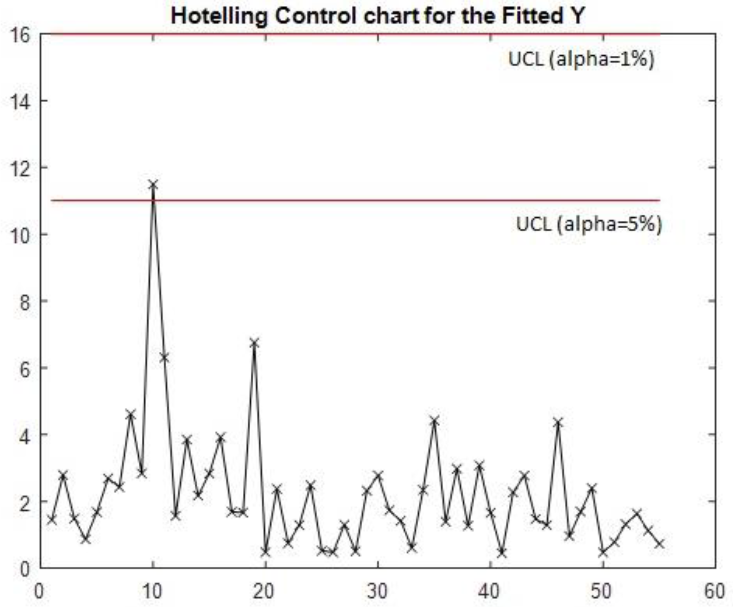
Figure 3.
Hotelling’s T2 control chart for predicted observations of Y. This version uses the in-control covariance matrix to estimate Hotelling’s T2 statistic.
Figure 3.
Hotelling’s T2 control chart for predicted observations of Y. This version uses the in-control covariance matrix to estimate Hotelling’s T2 statistic.
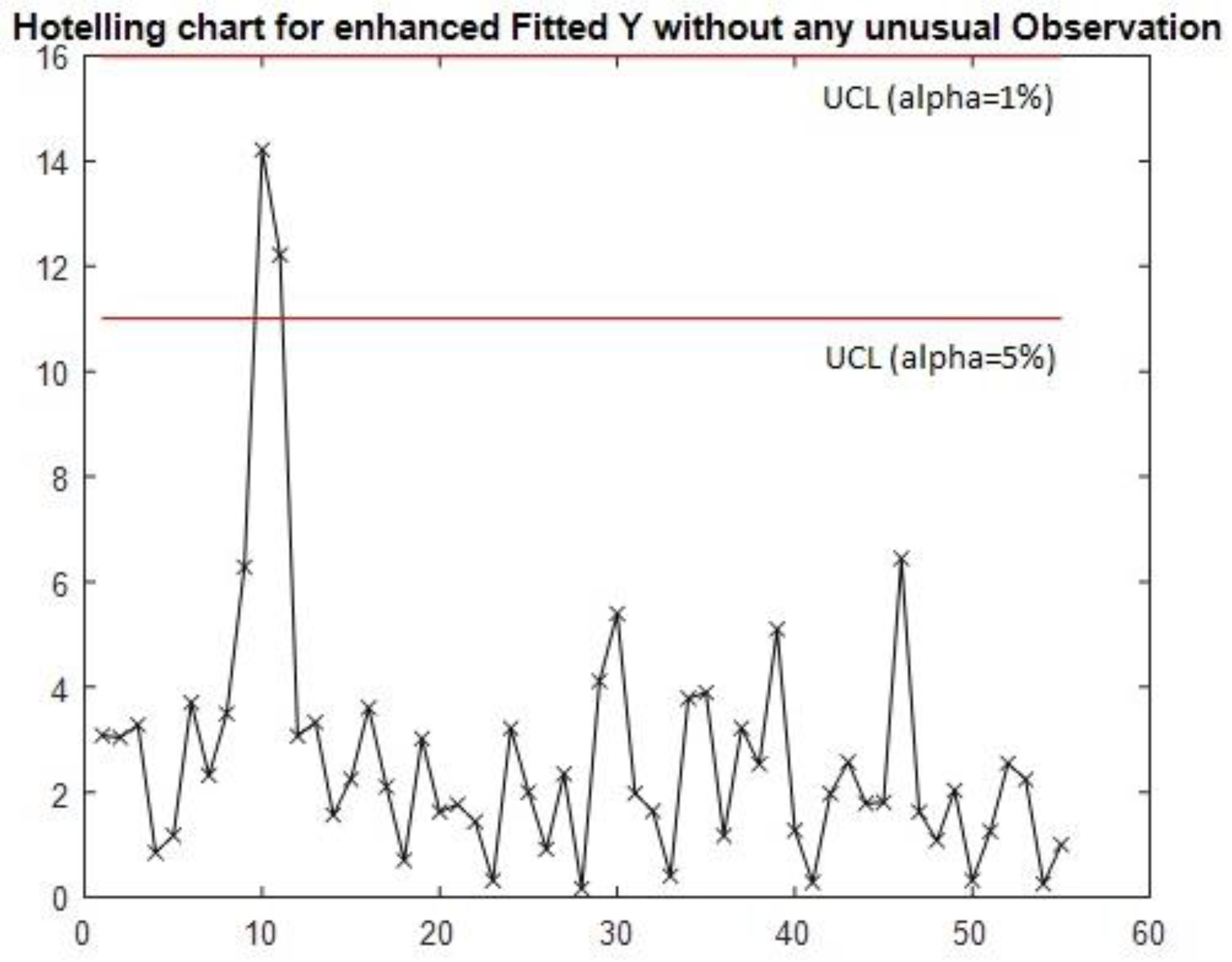
Figure 4.
Hotelling’s T2 control chart of X (input data matrix).
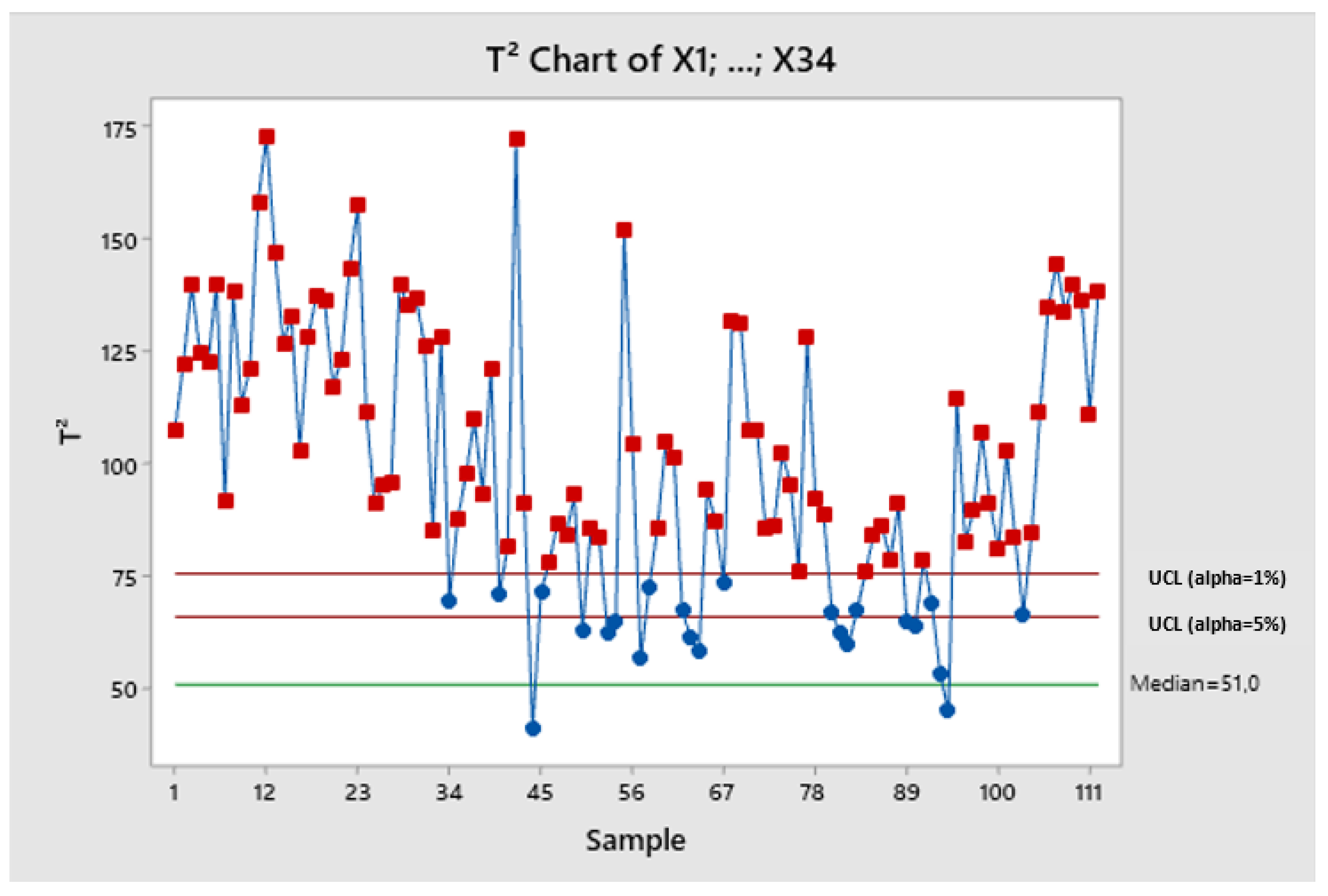
Figure 5.
Univariate control chart for predicted values of y3.
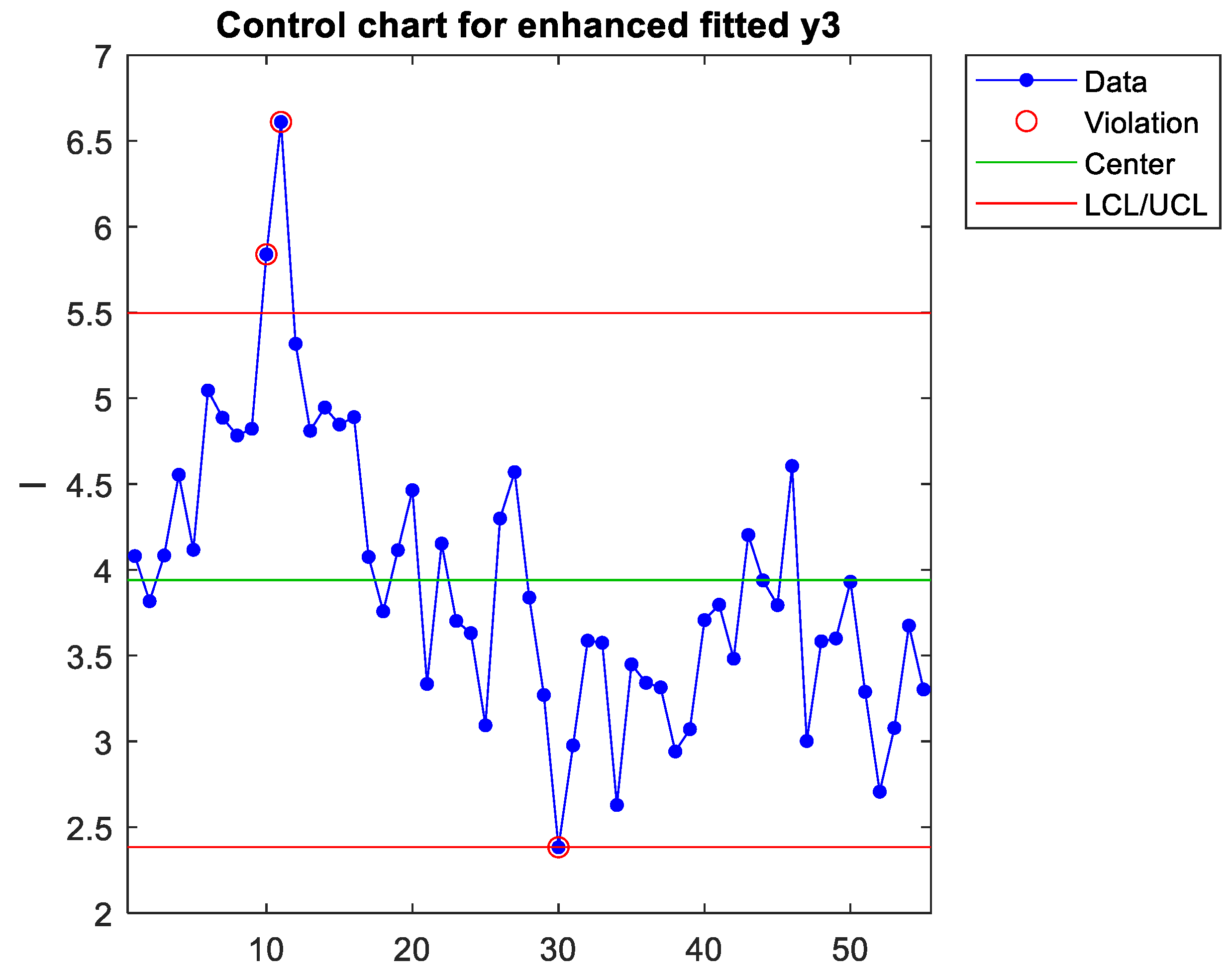
Figure 6.
Control chart of X scores for the first component (latent variable).
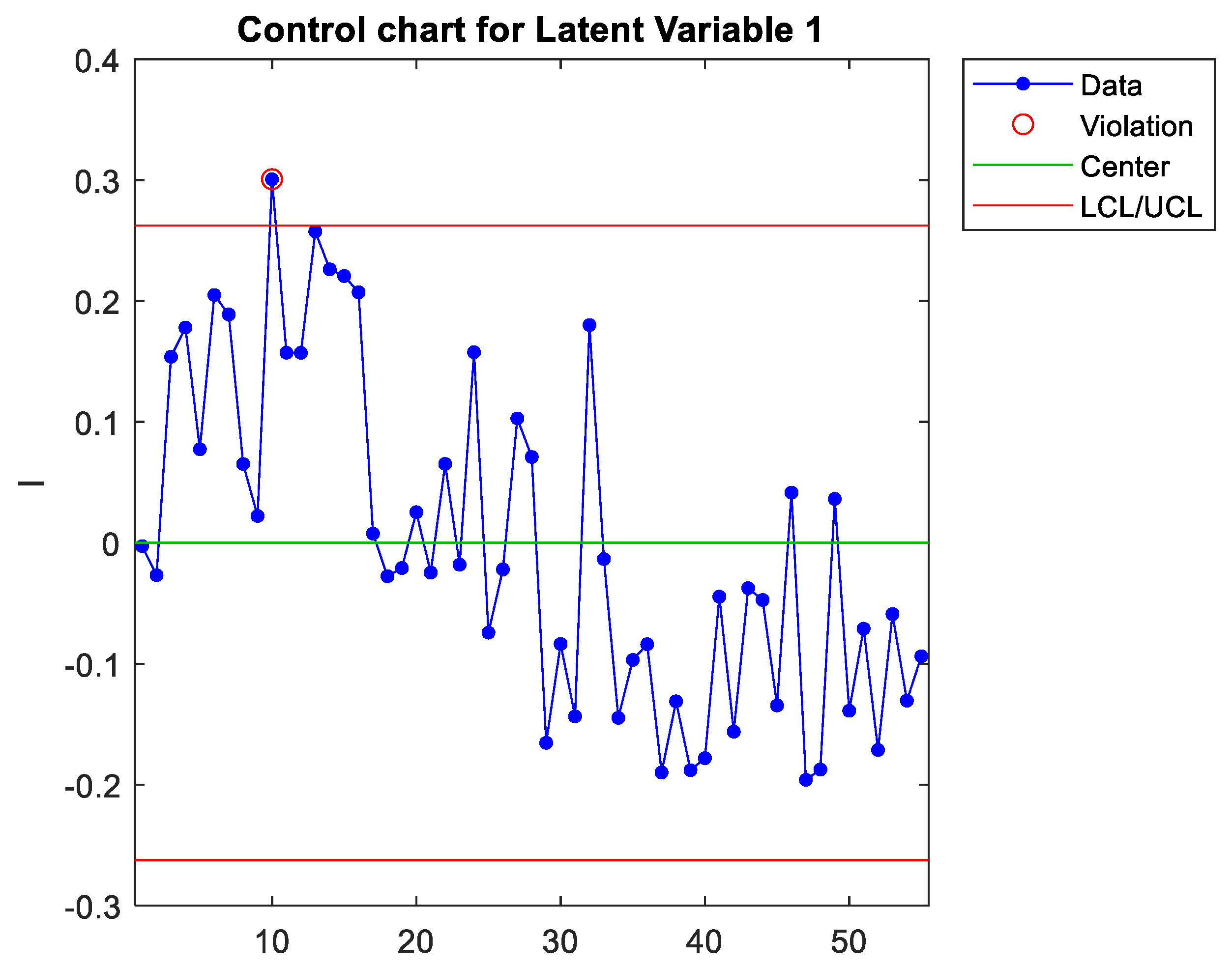
Figure 7.
Factor weights for the first component (latent variable) of predicted y3.
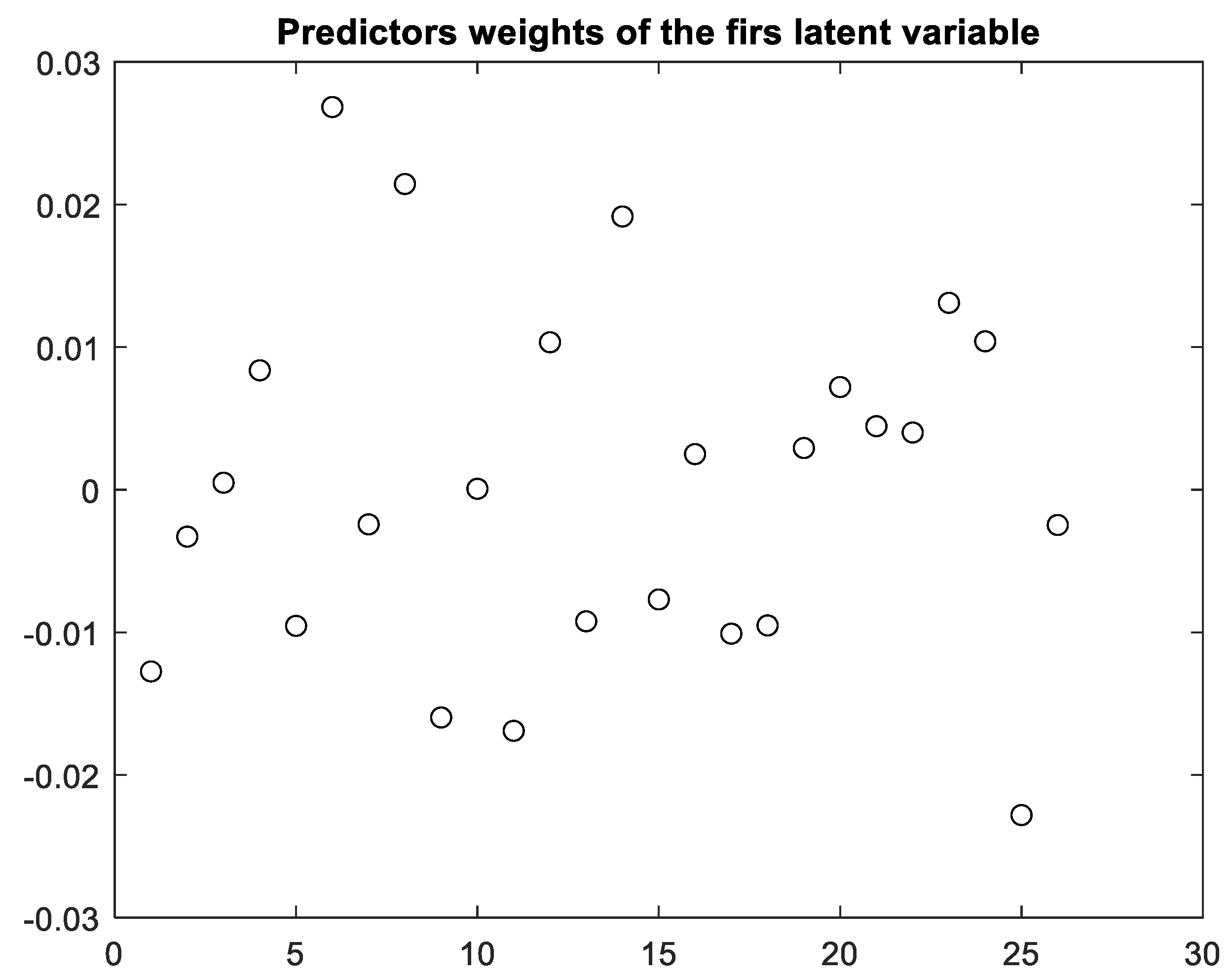
Figure 8.
Control chart for x6 (real variable).
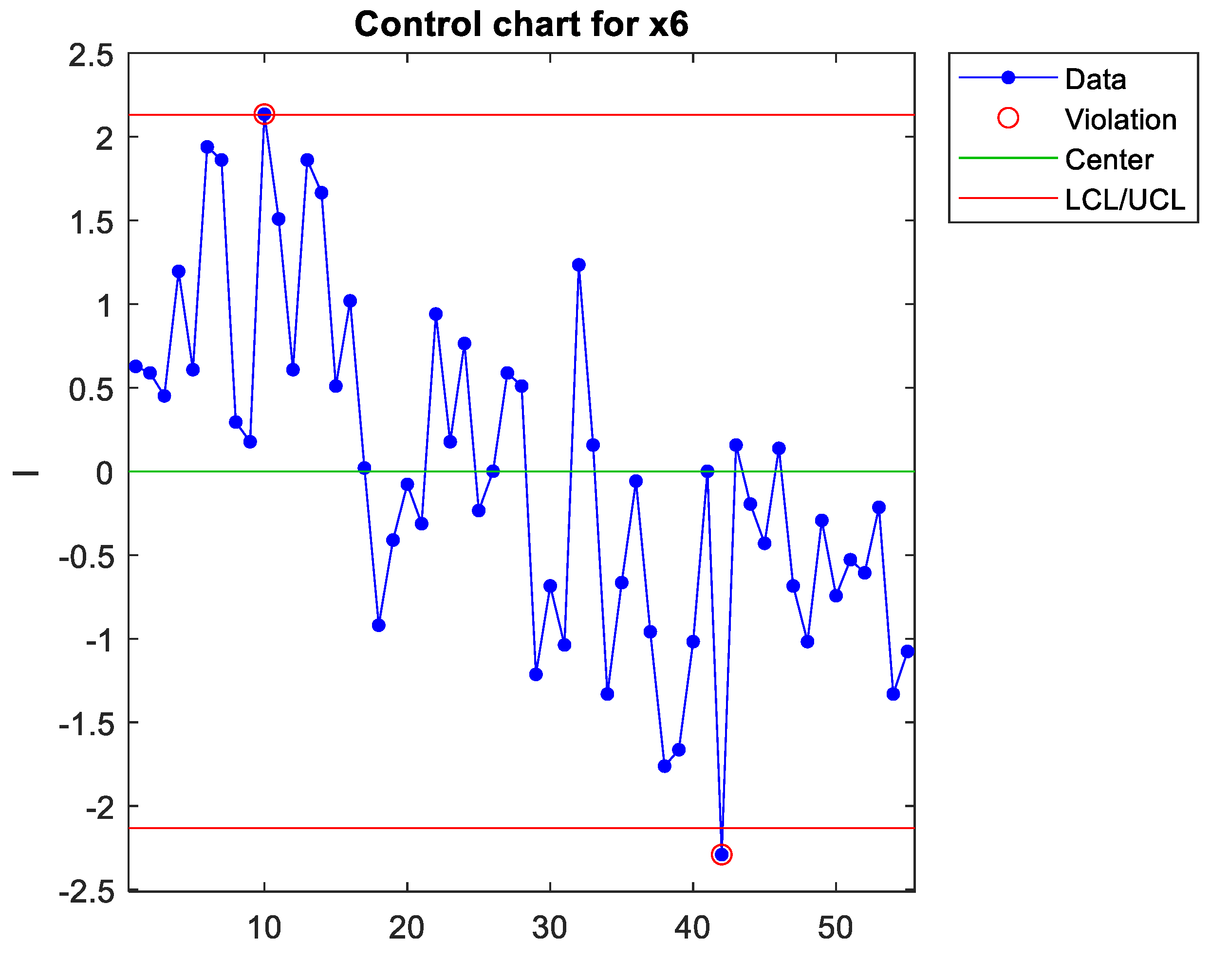
Figure 9.
Control chart for the projection onto latent variable 1 of x6, x8, x9, x11, x14 and x25.
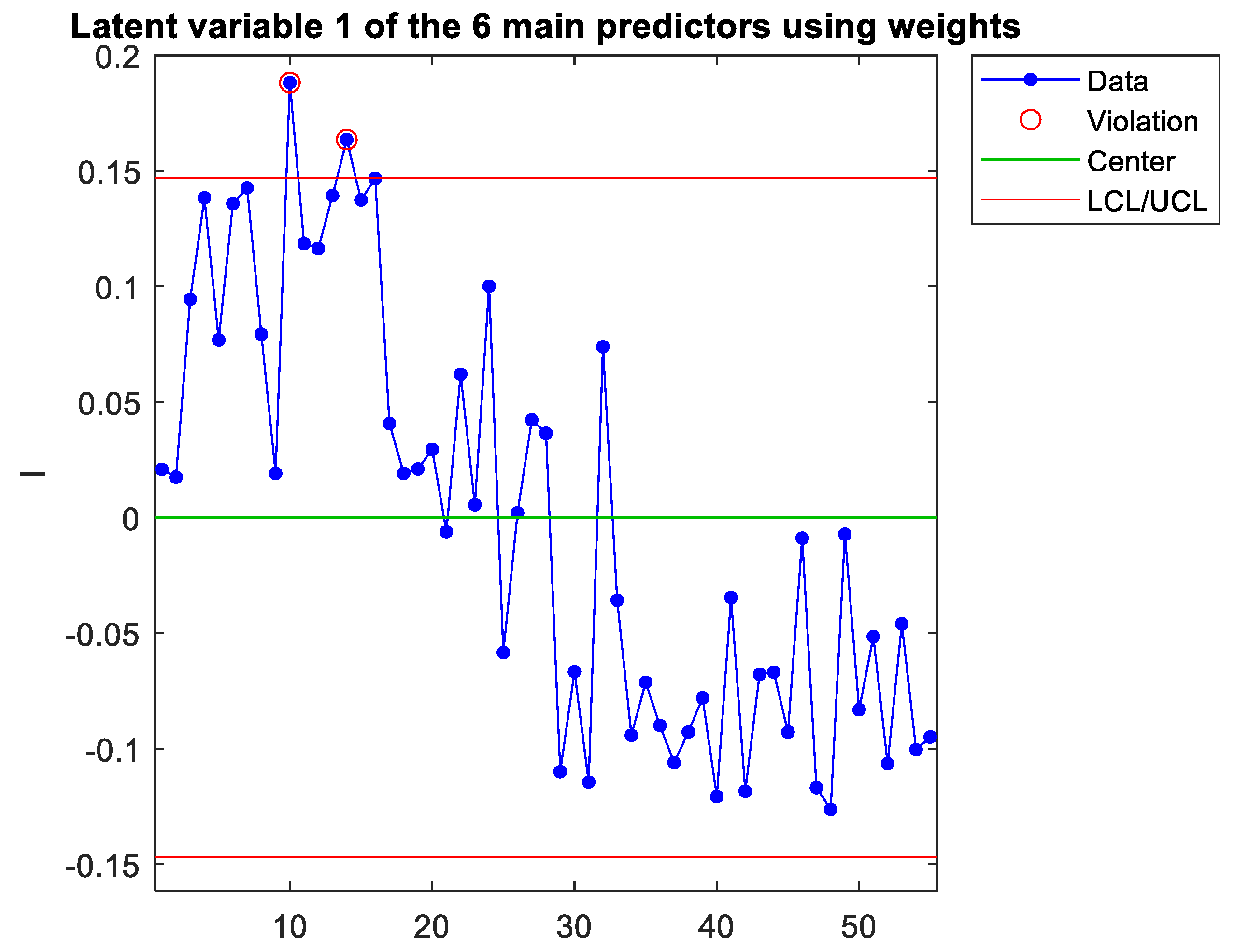

Table 1.
R2 for each of the four output variables obtained by one PLS model (regressing X onto the four output variables at the same time).
Table 1.
R2 for each of the four output variables obtained by one PLS model (regressing X onto the four output variables at the same time).
| Variable | y1 | y2 | y3 | y4 |
| R2(%) | 52.616 | 54.364 | 65.296 | 43.395 |
Table 2.
R2 for each of the four output variables obtained by four separate PLS models (regressing X onto the four output variables one by one).
Table 2.
R2 for each of the four output variables obtained by four separate PLS models (regressing X onto the four output variables one by one).
| Variable | y1 | y2 | y3 | y4 |
| R2(%) | 64.876 | 59.791 | 77.446 | 54.958 |
Disclaimer/Publisher’s Note: The statements, opinions and data contained in all publications are solely those of the individual author(s) and contributor(s) and not of MDPI and/or the editor(s). MDPI and/or the editor(s) disclaim responsibility for any injury to people or property resulting from any ideas, methods, instructions or products referred to in the content. |
© 2025 by the authors. Licensee MDPI, Basel, Switzerland. This article is an open access article distributed under the terms and conditions of the Creative Commons Attribution (CC BY) license (http://creativecommons.org/licenses/by/4.0/).
Copyright: This open access article is published under a Creative Commons CC BY 4.0 license, which permit the free download, distribution, and reuse, provided that the author and preprint are cited in any reuse.


