
Submitted:
12 December 2024
Posted:
18 December 2024
You are already at the latest version
Abstract
Classical Partial Least Squares (PLS) models were developed primarily for continuous data, allowing dimensionality reduction while preserving relationships between predictors and responses. However, their application to binary data is limited. This study introduces Binary Partial Least Squares (BPLS), a novel extension of the PLS methodology designed specifically for scenarios involving binary predictors and responses.
Keywords:
partial least squares
; binary data
; biplot
; NIPALS
1. Introduction
Due to the great technological advances nowadays, it is increasingly common to find datasets that contain a large number of variables that have been measured in a given sample. The set of variables can range from quantitative to binary, nominal or ordinal and, very often, a combination of several types.
The rapid growth of data science has led to an increasing demand for statistical techniques that can handle large and complex datasets.
In this context, traditional univariate statistical techniques, repeated for each variable, do not capture the structure of the data, specially the relationships among variables, so it will be necessary to use multivariate techniques that offer a more powerful approach. These methods focus on the study of relationships among variables, similarities and differences among individuals and the variables responsible for them, treating all available information simultaneously.
Probably the most used multivariate statistical technique is Principal Components Analysis (PCA). Pearson [1] proposed PCA over 120 years ago, which was later formalized by Hotelling [2], Hotelling [3]. PCA is a dimensionality reduction technique that can be used to summarize the information contained in a large dataset. PCA works by finding a set of orthogonal axes, called principal components, that capture the most variation in the data. It was not until a few years later, in 1971, that K.R. Gabriel [4] proposed a simultaneous graphical representation of the rows and columns of a data matrix, related to PCA, which he called biplot.
This type of methods will allow for visualizing the structure of the data, avoiding making use only of a list of p-values associated with the performed analysis. Biplots can also allow the visualization of more complex multivariate models as Canonical Variate Analysis or Multivariate Analysis of Variance (MANOVA) [5,6,7].
All of these techniques were developed for continuous variables, but when the measured variables are of a categorical type, either binary, nominal or ordinal, these representations are not adequate.
There are several dimension reduction methods for categorical data, for example Item Response Theory (see for example [8]) or Factor Analysis for categorical data (see for example [9]), but none of these techniques had an associated biplot representation.
We will focus here on biplot representations based on logistic responses that are closely related to the mentioned techniques. It is worth highlighting the work of Vicente-Villardon et al. [10], Demey et al. [11] who have developed a biplot for a single matrix of binary data, Hernández-Sánchez and Vicente-Villardón [12] for nominal data, Vicente-Villardón and Hernández Sánchez [13] for ordinal data and Vicente-Villardón and Hernández-Sánchez [14] who have developed a biplot for mixed data that contains several types of variables. These proposals are based on the generalized bivariate models proposed by Gabriel [15].
In many practical situations, we have two or more data matrices, with symmetric or asymmetric roles. In this work, we focus on the particular case in which we have two data matrices with asymmetric roles, a set of predictor variables and a set of response variables. Generally, the goal when we have this situation is to find models that allow predicting the responses from the predictors. In both data sets, it is possible to have variables of all the types mentioned above.
For two multivariate data matrices with one playing the role of responses, one of the most used multivariate statistical techniques is Partial Least Squares (PLS) [16,17]. PLS is a regression technique that can be used to predict a set of response variables from a set of predictor variables. PLS works by finding a set of linear combinations of the predictor variables that are most correlated with the response variables. The classical PLS models were developed mainly for continuous data and obtain dimension reductions in both, the responses and the predictors, in a way similar to PCA with the difference that the focus is on prediction rather than variance maximization. A biplot representation for PLS that can help in the interpretation of the results was proposed by Oyedele and Lubbe [18].
More recently, Vicente-Gonzalez and Vicente-Villardon [19] proposed a PLS method when all the responses are binary and predictors are continuous. This extended PLS generalized linear regression [20] for a single response variable (PLS1) to several responses (PLS2) in a non-trivial way because it imply a dimension reduction not present in the former work. This proposal goes with a biplot for both matrices, a continuous one for the predictors and a logistic one for the binary responses.
When the two matrices are binary none of the mentioned procedures are suitable. In this paper we propose a PLS (PLS2) procedure when both matrices, responses and predictors, have binary variables. We use the logistic biplots, mentioned before, to make a triplot representation that combines individuals and variables of the two initial matrices.
The database that initially motivated the development of this method is studying the relation among origin of 9 types of corn strains and the presence or absence of genes. The data is composed of two binary matrices, the first one containing indicators of the 9 classes and the second a set of binary genetic polymorphisms.
2. Partial Least Squares
Let be a matrix of predictors with J variables and be a matrix of responses with K variables, both measured in I individuals.
When we have only a few predictors (significantly fewer than the number of individuals) that are not strongly correlated, multivariate linear regression (MLR) is typically employed to predict the responses. However, when the predictors are highly collinear or when there is a large number of them, traditional linear regression models may be inadequate.A notable example occurs when the number of observations is significantly smaller than the number of predictors, resulting in the absence of parameter estimates for MLR. This situation commonly arises in genomic studies, where a set of gene expressions is used to predict tumor types.
Partial Least Squares (PLS) [16,17] is one of the most recognized and widely applied methods for modeling the relationships between two datasets, particularly when both sets of variables are continuous and the MLR is not suitable.
Traditionally, this technique is used for prediction, but it lacks a graphical representation to help interpret the relationships between the two sets. When the responses are continuous, Oyedele and Lubbe [18] introduced an associated biplot representation, although earlier, less formal versions exist, such as in [21]. More recently, PLS-Biplot has been applied to team effectiveness [22].
When the response matrix contains binary variables, Partial Least Squares Discriminant Analysis (PLS-DA) [23] is often employed, which essentially fits a PLS regression to a dummy or fictitious variable. Bastien et al. [20] introduced a PLS model for a single binary response, analogous to the PLS-1 model. More recently, Vicente-Gonzalez and Vicente-Villardon [19] proposed a non-trivial extension for multiple binary variables, incorporating dimension reduction for binary data and resulting in a PLS-2 model, which serves as an alternative to PLS-DA.
In regression, to address the discriminant problem, Logistic Regression (LR) can be used instead of Multivariate Linear Regression, allowing the binary nature of the responses to be captured. While this is often a valid approach, LR faces the same limitations as MLR regarding the number of individuals, variables, and collinearity. Additionally, the separation problem may also arise.
Currently, no PLS alternative exists for situations where both the predictor and response matrices are binary.
The aim of this section is to extend PLSR to cases where both the predictor and response matrices consist of binary variables, by using logistic functions instead of linear ones. This approach, referred to as Binary Partial Least Squares (BPLS), enables us to account for the binary nature of the responses and addresses the limitations of traditional PLS methods when dealing with binary data.
This generalization is based on the adaptation of the NIPALS algorithm for binary data proposed in previous works by Vicente-Gonzalez and Vicente-Villardon [19]. The adaptation consists of replacing the linear regression step in the NIPALS algorithm by a logistic regression step. This allows the procedure to capture the binary nature of the data. Previously we make an outline of the classical PLS-2 model.
2.1. Partial Least Squares Regression: NIPALS Algorithm
PLS seeks to identify linear combinations of continuous predictors that optimally predict a set of continuous responses . Here, we outline the classical NIPALS algorithm [24]. Both sets are usually column-centred and probably standardized. PLS operates by extracting latent variables that capture the most significant variance and covariance between predictors and responses. It uses iterative extraction of components to build a predictive model that can handle collinearity and high-dimensional data effectively.
The latent model for predictors , in S dimensions, is
where are variable loadings, are scores for individuals and is a matrix of residuals.
In the same way the latent model
where are loadings, are scores and are residuals.
Observe that both models share the matrix of scores that best predict the responses. The NIPALS algorithm to obtain the parameters can be described as follows:
| Algorithm 1 (NIPALS Algorithm) |
|
Note that by removing the step where predictors are updated in the NIPALS algorithm, we would end up with the principal components for the responses. The procedure alternatively updates the scores in matrix using the information of responses and predictors.
Here, and , and contains the scores from that best explain the set of responses. We have the relationship:
A potential issue with this and subsequent algorithms is that they may have multiple starting points, leading to different solutions. The algorithm generates sequences of decreasing residual sum of squares values and eventually converges to at least a local minimum.
If we need the regression coefficients to express the variables as functions of the predictors , we have
Considering that , we have
Thus, the regression coefficients in terms of the original variables are
We have to note that the updating steps in the Algorithm 1 minimize the sum os squares of the residuals that can also be understood as a lost function.
for the responses and in a similar way for the predictors.
2.2. PLS for Binary Responses
When responses are binary, the updating steps of the NIPALS algorithm (steps 7 and 8) are inadequate because the implicit linear relationship it assumes is not adequate. This is similar to how linear regression is unsuitable for binary responses, with logistic regression being the more appropriate method. The difference in step 11 makes also no sense.
Recently, Vicente-Gonzalez and Vicente-Villardon [19] generalized the NIPALS algorithm to handle a set of binary responses by incorporating a logistic relationship with the latent variables.
The expected values for the responses are now probabilities, and we use the logit function as the link function. Let , then we have:
This equation generalizes equation (2), except that we need to include a vector with intercepts for each variable, as binary variables cannot be centred in the same way as continuous. Each probability can be expressed as
Or in matrix form, if we have
then
where the operations apply to each element of the matrices.
The updating steps of the responses have to be changed for binary responses. Rather than minimizing the cost function in Equation (7) we minimize the cost defined as
We interpret here the function as a cost to minimize rather than a likelihood to maximize. We look for the parameters , and that minimize the cost function. There are not closed-form solutions for the optimization problem so an iterative algorithm in which, we obtain a sequence decreasing values of the lost function at each iteration, is used. We will use the gradient method in a recursive way calculating one component at each time fixing the previous one. The update for each parameter would be as follows:
for some . Or, in matrix form
| Algorithm 2 (NIPALS-Binary responses) |
|
In practice, the choice of can be avoided by using a pre-programmed optimization routine. This algorithm is implemented in the package MultBiplotR [25] developed in the R language [26].
In the same way as for the continuous case, the regression coefficients in terms of the original variables are
Algorithm 2 is essentially the same as algorithm 1 except that we have made the necessary adaptations to cope with binary responses. Now, the relation between the manifest and latent variables is logistic rather than linear. Observe that is also a linear relation on the logits, i. e. a generalized linear model.
2.3. Partial Least Squares for Two Binary Matrices
Now both and contain binary variables measured in the same I individuals. The goal is still predicting from and describing the common structure of predictors and responses.
We denote the expected values of as and the expected values of as . Then we have
and
These Equations are generalizations of the decompositions of the matrices and for the continuous case in Equations 1 and 2. The only difference is that we need to add the intersection vector for each variable ( and respectively). This is because, unlike the continuous case, the variables cannot be centered beforehand.
The relation among observed and latent variables, can be written as:
That is, a logistic rather than linear relation.
Now, we have to design an algorithm to calculate the model parameters. The procedure alternatively updates the common scores in using the information of responses and predictors. We use the gradient method and the lost functions as follows
and
We will update the scores using a gradient descent procedures as in Equations (16), (17) and (18) for the responses. The extension for predictors in is straightforward.
2.3.1. NIPALS Algorithm for Two Binary Matrices
Then, we will search for the parameters , y for the predictors and , y for the responses. We will obtain the scores for that better predict with a logistic regression model. The scores are also related to predictors with a logistic response model.
The calculations can be organized in an alternating algorithm that calculates the parameters , and for each dimension s, while fixing the parameters already obtained in the previous dimensions. First, we need to calculate the constant (dimension 0) and separately. This is so because data can not be centered before hand.
The algorithm is as follows.
| Algorithm 3 (PLS for two binary matrices - BPLS) |
|
In logistic regression, there is a potential problem known as separation. This occurs when the data are perfectly separable by a linear combination of the predictors. In this case, the maximum likelihood estimator does not exist and tends to infinity [29]. Even if the separation is not perfect (quasi-separation), the estimator can be highly unstable.
To avoid separation, the usual solution is to use a penalized likelihood [30]. This adds a penalty term to the likelihood function that encourages the coefficients to be smaller. In our case, we will use the Ridge penalty [31].
Gradient adaptation for the penalized cost function is automatic:
To address the separation problem, we can introduce a regularization parameter . This parameter penalizes large coefficients, making the solution less likely to be separated.
The BPLS algorithm (Algorithm 3) can be sensitive to the random start. To obtain the best possible solution, it is recommended to test several starting points. In practice, it has been observed that the solutions from different starting points produce similar predictions of the responses.
The BPLS algorithm can also suffer from the separation problem.
If we eliminate the part where and are updated in algorithms 3 and 2 we obtain a reduced dimension approximation of a single data matrix analogous to a multidimensional logistic two parameter model in Item Response Theory, see [32,33]. It is also similar to Principal Components Analysis for binary data as in [34,35,36,37], or to Factor analysis for binary data [9].
3. Biplots
A biplot [4] is a type of graph that simultaneously displays two sets of information: the scores of the observations and the loadings of the variables in a reduced-dimensional space. It is commonly used in techniques like Principal Component Analysis (PCA) and Partial Least Squares (PLS) regression, among many others, to visualize high-dimensional data in two or three dimensions.
Scores represent the projections of the original data points (observations) onto a reduced number of components or latent variables. Loadings indicate the contributions of the original variables to these components, showing how each variable relates to the reduced dimensions.
In a biplot, observations (samples) are often represented by points, while the loadings (variables) are shown as vectors (arrows). The angles and lengths of the arrows help interpret how variables are correlated and how they contribute to the variation in the data.
Formally, a biplot represents the approximate decomposition of a data matrix into the product of two lower-rank matrices (typically two or three), as follows:
This decomposition approximates the original matrix as accurately as possible based on specific criteria, with and capturing the main structure and representing the residuals or error. In fact, a biplot decomposes the expected approximate structure of the data matrix into the product of two other matrices. The matrix captures the majority of the data’s characteristics based on a predefined criterion.
Matrices and can be represented as points into a two or three dimensional space in such a way that the inner product
approximates the element .
Biplots were initially proposed in connection to PCA [4] but have been used also accompanying other techniques as Multivariate Analysis of Variance (MANOVA) [5,6,38], STATIS-ACT [39], Correspondence Analysis [40] among many others. In the context of PLS for continuous data it is clear that Equations (1) and (2) define a biplot. The properties of those representations can be developed by Oyedele and Lubbe [18] and Vicente-Gonzalez and Vicente-Villardon [19].
Most biplots are based on the assumption of linear relationships between observed and latent variables and are primarily designed for continuous data. For binary data, however, these representations are not ideal, much like how linear regression struggles to accurately model relationships with a binary response.
Vicente-Villardon et al. [10] introduces a method where the relationship between the observed variables and the dimensions is modeled using a logistic approach. This method is linked to psychometric techniques, such as item response theory or latent trait analysis. The original paper proposes an algorithm based on alternating generalized regressions using the Newton-Raphson method to maximize the likelihood. However, the algorithm faces the same challenge as logistic regression when separation occurs. Specifically, for some binary variables, individuals displaying the presence of a characteristic are fully separated from those without it (by a hyperplane) in the final representation. This method is referred to as the Logistic Biplot.
Demey et al. [11] introduced a new algorithm that combines Principal Coordinates Analysis, Cluster Analysis, and Logistic Regression to create this type of biplot. The result is termed an "external logistic biplot" because it uses a two-step approach (Principal Coordinates for individuals and Logistic Regressions for variables) rather than simultaneously obtaining the row and column markers. This simplification helps to avoid the separation problem but comes at the cost of reduced goodness of fit.
More recently, Babativa-Márquez and Vicente-Villardón [41] proposed an algorithm that improves parameter fitting by employing the nonlinear conjugate gradient algorithm.
More recently, in the context of PLS methods, Vicente-Gonzalez and Vicente-Villardon [19] proposed a generalization of the NIPALS algorithm for binary responses, where the components are obtained iteratively using the gradient method. The paper also introduces a procedure to address the separation issue encountered in earlier algorithms for logistic biplots.
3.1. Logistic Biplots
Linear biplots decompose the expected values of the approximation into a product of two lower-rank matrices. In contrast, the logistic biplot decomposes the expected probabilities using the logit link function, similar to how generalized linear models operate.
For any binary data matrix , if we call the decomposition, using the logit link, is
The constants have to be included because data can not be centered beforehand as in the continuous case. With this decomposition, the inner product of the biplot markers (coordinates) is the logit of a expected probability, except for a constant,
The logits are easily converted into probabilities
Then, by projecting a row marker onto a column marker we obtain, except for a constant, the expected logit and thus the expected probability for the entry of . The constant serves to determine the exact point where the logit is zero or any other value.
Due to the generalized nature of the model, the geometric interpretation closely resembles that of linear biplots. Computational procedures are analogous to those employed in previous cases, with the addition of the constant term. For example, in two dimensions, we can determine, on the direction of the vector , what point predicts a given probability p. Let’s that point, satisfying the equation
Prediction also verifies that
Therefore, we obtain
The point in the direction of that predicts (), is
Using Equations (33), we can position markers for different probabilities along the direction of , creating a graded scale similar to a coordinate axis. The interpretation remains fundamentally similar to that of linear biplots; however, markers representing equidistant probabilities may not be spaced equally in the graph.
As an illustrative simple example with data taken from [42]. The data companies collect can include the expected, such as your name, date of birth, and email address, as well as more unusual details, such as your pets, hobbies, height, weight, and even personal preferences in the bedroom. They may also store your banking information and links to your social media accounts, along with any data you share there.
How companies use this data varies depending on their business, but it often leads to targeted advertising and optimizing website management.
The infographics taken from the site is shown in Figure 1. The picture shows information on your face, voice, and environment, that some internet companies collect.
The original data has been transformed into a binary matrix, where the rows represent internet companies, the columns represent the types of information collected, and each entry is marked as 1 if the company collects that information, and 0 if it does not. The data matrix is shown in Table 1. With this data we have performed a Logistic Biplot that summarizes the information in a two dimensional graph. We obtain a joint representation of rows and columns of the data matrix. Distances among companies will be interpreted as similarities, i. e., companies lying near on the biplot display have similar profiles in relation to the collected information. Angles between variables (kind of information) is interpreted as correlations. Acute small angles mean strong positive correlations, near straight angles, strong negative correlations and almost rights angles mean no correlation. Projecting the row markers onto column markers, we have the expected probability for each entry.
Figure 2 shows the graphical results as a typical logistic biplot with scales for probabilities 0.05, 0.25, 0.5, 0.75 and 0.95. We have used percents (5, 25, 50, 75, 95) rather than probabilities to simplify the plot. We could have used any other values for the probabilities.
The plot displays a two-dimensional scattergram, where points represent the rows (companies) of the data matrix, and vectors or directions correspond to the variables. Distances among points for companies are inversely related to their similarity, for example, points representing Facebook, Instagram and Tik-Tok coincide, indicating that the three companies have exactly the same profiles (the three collect all the available information). Companies with a single point have unique patterns, for example, Offerup, Uber or eBay, and groups with close points have several characteristics in common.
As previously mentioned, the angles between the variable directions provide an approximation of the correlations between them. For example, face recognition, environment recognition and languages have high positive correlations because the increasing probabilities point into the same direction, i. e. have small acute angles between them. Collecting the contacts is not correlated to this group because they form an straight angle with it. Contacts and image library are negatively correlations because the probabilities increase in opposite directions.
The angles are connected to tetrachoric correlation due to the close relationship between this representation and the factorization of the tetrachoric correlation matrix, as we will explain later.
Projecting companies into the direction of a variable, we have the expected probabilities given by the approximation. Figure 3 shows the projections onto the variable "Face Recognition". The point predicting 0.5 has been marked with a circle because is usually the cut point to predict presence or absence of the characteristic.
To simplify the plot we can place marks for just a few probabilities, for example, 0.5 and 0.75 indicating the point were expected logit is 0 (probability 0.5) and the direction of increasing probabilities. Figure 4 shows a simplified logistic biplot with probabilities 0.5 and 0.75.
We can use the expected probabilities from equation (32) to generate predicted binary values: if and 0 otherwise. This yields an expected binary matrix . In the plot, this indicates that for each variable, the plane is divided into two prediction regions by a line perpendicular to the variable’s arrow and passing through the point predicting 0.5. The region on the side of the arrow predicts the presence of the characteristic, while the opposite region predicts its absence. Figure 5 illustrates this statement.
A guide for the interpretation of the biplot can be found also in the supplementary material by Demey et al. [11].
A common overall goodness-of-fit measure is the percentage of correctly classified entries of the data matrix. To assess the quality of representation for individual rows (individuals) and columns (variables), we can calculate these percentages separately. We can also calculate the percentage of true positives (sensitivity) and true negatives (specificity).
To evaluate the quality of representation for each binary variable, we need a suitable measure that generalizes the measures of predictiveness for continuous data as in [43]. Equation (32) essentially defines a logistic regression model for each variable when the row coordinates are fixed, that allows to evaluate goodness of fit using pseudo- measures commonly associated to that model, for example, McFaden, Cox-Snell or Nagelkerke.
Table 2 contains fit measures for the Internet Companies Data. It contains fit measures for each column separately and for the complete table.
94% of all entries in the data table are correctly predicted by the previously described procedure, as shown in Figure 5. However, it is more insightful to examine the indices for each individual variable. This is because, in some cases, only a few variables are accurately represented. Such a situation can arise when dealing with a large set of variables, where only a small subset is actually relevant to the problem. For instance, in a genetic polymorphisms matrix, only certain variables may be of real interest.
In our example, all variables show a reasonable percentage of correct classifications, except for "Image Library," which correctly classifies only 80% of all values and 66.67% of the negatives. Additionally, we included the deviance for each variable in the model, using the latent dimensions as predictors, along with a p-value as an indicator of model fit. This measure, potentially adjusted for multiple comparisons, could be used to select the most significant variables, as demonstrated in [11]. We also show pseudo- measures. All have high values except for "Image Library" and "Voice Recog." that are worse predicted or represented on the graph.
By assuming that the observed categorical responses are discretized versions of continuous processes, we can leverage the close relationship between the presented model and the factorization of tetrachoric correlations to perform a factor analysis.
Consider a binary variable . This variable is assumed to arise from an underlying continuous variable that follows a standard normal distribution. There is a threshold, , which divide the continuous variable into two categories.
The relationship between and can be expressed as:
The tetrachoric correlations are the correlations among the . Let a matrix containing the tetrachoric correlations among the J binary variables and let the thresholds.
We can factorize the matrix as
where contains the loadings of a linear factor model for the underlying variables.
It can be shown that there is a close relation between the factor model in Equation (34) and the model in Equation (32). You can find the details in [9]. The model in Equation (32) is actually equivalent to the multidimensional logistic two parameter model in Item Response Theory (IRT).
The factor model loadings and he thresholds can be calculated from the parameters for the variables in our model as:
In this way we provide a classical factor interpretation to our model adding the loadings and communalities (sum of squares of all dimension loadings of each variable). Loadings measure the correlation among the dimensions or latent factors and the communalities the amount of variance of each variable explained by the factors. For our data, the loadings and communalities are in Table 3.
The two dimensional solution explains the 88% of the variance. All the comunalities are higher than 0.71 meaning that a good amount of the variance is explained by the dimensions. The communalities serve also to select important variables. Variables with low communalities may be explained by other dimension or have little importance for the description of the rows.
We can see also that Face Recognition, Environment Recognition and Language, are mostly related to the first dimension while, Product Recognition, Your contacts are related to the first dimension. Voice Recognition is related to both.
3.2. Triplot Representations for Binary Partial (Least Squares) Regression
Equations (1) and (2) define two biplots for the continuous case that share the scores for individuals in . Some of the properties of those biplots have been described by Oyedele and Lubbe [18].
In the same way, Equations (1) and (8) define two biplots that share scores in but now the biplot for responses is a logistic biplot as described in subSection 3.1. The details of this representation can be found in [19]. For this case, Equation (19) defines a biplot for the regression coefficients in terms of the observed variables that can help in determining the more important predictors to explain the responses.
The Equations in (20) and (21) define two logistic biplots with the particularity that both share the row scores in . We can plot those together with the loadings for responses and predictors to obtain a joint representation of individuals, responses and predictors, i. e. a triplot with three sets of markers. Both biplots and then, the triplot, are interpreted using the rules in subSection 3.1.
The measures of quality (Correct classifications, sensitivity, specificity, pseudo-, factor loadings or communalities) for matrix can be used to identify which responses are correctly explained and what dimensions are needed for the explanation. Global qualities can be used to determine the number of dimensions needed for an adequate prediction, taking into account that some of the responses may not be well predicted by the model. In this case angles among directions for responses or projections of the scores on them are less important because are not optimized to explain the variability in data but to capture the relations with the predictors. The same occurs for the joint interpretation of rows and columns
4. Illustrative Example
Anderson et al. [44] estimates that approximately 30% of plant diseases are caused by phytopathogenic fungi. These fungi can have a significant impact on both ecology and agriculture, causing crop losses and environmental damage.
We focus on a specific fungus, Colletotrichum graminicola (or Glomerella graminícola). This fungus is a major pathogen of corn, causing a disease called anthracnose. Anthracnose produces spots on the leaves and stems of corn plants, which can lead to crop losses. There are some studies, such as that of O’Connell et al. [45], which collect the economic impact it had in the United States.
The data used in this study comes from a project carried out by the CIALE. The project collected samples of corn plants infected with Colletotrichum graminicola from 9 different countries: Argentina (AR), Brazil (BR), Canada (CA), Croatia (HR), Slovenia (SI), France (FR), Portugal (PT), Switzerland (CH) and the United States (US). The response matrix has the indicators (dummy variables) for the countries,
The predictors are a set of binary polymorphisms obtained from the RNA sequencing of the fungus Colletotrichum graminicola yielded a total of 13,183 variables. However, the sequencing method generates duplicate information, a variable for the presence and another for the absence, that are complementary; so we first removed those variables for the absence. This reduced the number of variables to 6,419. We then selected the 2,379 variables that were most significant based on their correlation with the response variable, i.e., the presence or absence of anthracnose.
The statistical analysis was carried out with the statistical software R [26]. We used the MultBiplotR package [25], which includes functions for performing the proposed method including biplot analysis.
The biplot representation of the responses is shown in Figure 6. Rather than the rows, the convex hulls containing all the points of each origin, have been represented.
The BPLS model achieved an overall classification accuracy of 90.94% considering the binary variables separately. The classification accuracy for each country, together with some additional measures of fit are shown in Table 4.
In our example, the strains from Brazil correctly classify all of their individuals. The rest have lower percentages of correct classification. Argentina, Croatia, France, Portugal and Slovenia have 0% Sensitivity, that is none of the presences is correctly classified. Switzerland has a sensitivity of 22.22 %. This kind of classification is more useful when we have several (possibly) correlated variables rather than a set of indicators for several classes.
In his particular case, in which we have the indicators of some disjoint classes, we can calculate another classification assigning each individual to the class with higher expected probability. The results of this classification are shown in Table 5.
With this classification only 49.51% of the strains are correctly classified into their origin. All the strains from Brazil, Canada, and France are correctly classified, but the strains from the USA are mistakenly grouped with those from Canada, while the remaining strains (Argentina, Croatia, France, Portugal, Slovenia, and Switzerland) are classified under France. This likely suggests that the characteristics of all European varieties (including Argentina) are quite similar, while Canada and the USA also share many similarities, with only Brazil showing distinct genetic characteristics. Experts have informed us that the Argentinian strains originated in Europe, which further supports this observation.
We have not included the predictors and its interpretation in this plot because of the big amount. We will show the interpretation in the next step of the analysis.
In conclusion we identify three groups with different genetic profiles according to the origin of the strains: Brazil, North America (USA, Canada) and Europe (Argentina, Croatia, France, Portugal, Slovenia, and Switzerland). We repeat the analysis recoding the whole set into those groups named: Brazil, North America and Europe (including Argentina).
The biplot for the new responses are in Figure 7. It is quite clear that all the groups are correctly classified.
Table 6 contains measures of fit for the responses. All measures are very high so no further comment is needed.
Table 7 contains the loadings and the comunalities that are very high for this data what means that the relations among the latent variables with the responses is very high.
The procedure is also helpful in identifying the variables that contribute to the prediction by examining the predictors most strongly associated with the latent variables used for prediction. We can add the predictors to the previous biplot to obtain a triplot. The resulting plot is shown in Figure 8.
Due to the high number of predictors the complete plot is too crowded and difficult to see and we may select just one fraction of the variables. We can use for example predictors that have high comunalities, or any other measure of fit.
We are interested in the predictors that point in the direction of each response and are highly related to the latent variables. For example, we can calculate the squared cosines between the directions of predictors and response to identify the most important polymorfisms for each group. Those cosines are easily calculated from the matrices in Equation (20). If the vector contains the lengths of the row vectors of (directions of predictors on the plot) and contains the lengths of the row vectors of (directions of responses on the plot), where the exponents apply to each element of the matrices, then the cosines are in the matrix
where and are the diagonal matrices with the lengths in the diagonal. Each column of contains the cosines of all the predictors with a single response, the near are cosines to 1 or -1, the closer are the direction of responses and predictors.
For each group we select the variables that have squared cosines higher than 0.9 and communalities higher than 0.85 to select also those related to the latent dimensions. The limits for the selection can be changed to select more or less predictors.
Figure 9 shows the variables most related to the direction that predicts Brazil and Table 8 the goodness of fit.
Figure 10 shows the variables most related to the direction that predicts Europe.
The number of variables highly associated with European tribes is significantly lower than those observed for Brazilian or American tribes. Nevertheless, the goodness of fit, as shown in Table 9, remains robust. Interestingly, all genes are directly related to the response variable, except for gene "409898", which shows an inverse relationship. Notably, this gene has a higher goodness of fit compared to the rest, highlighting its distinct contribution to the model. However, it is worth noting that the classification performance for the European strains does not reach the near-perfect results observed for Brazil. In particular, the percentage of cases correctly classified, as well as the sensitivity and specificity, do not reach 100%. This indicates a slightly lower overall predictive accuracy when analyzing the European dataset compared to the Brazilian one.
Figure 11 shows the variables most related to the direction that predicts North America.
The number of genes associated with the North American strain is significantly higher than those associated with the European and Brazilian strains. Only 10 genes are directly associated with the North American strain, while the rest have an inverse relationship with the response variable. The goodness of fit, as shown in Table 10, is high, indicating robust model performance. Nevertheless, the percentage of correctly classified cases does not reach 100%. Interestingly, in certain cases, either sensitivity or specificity achieves perfect accuracy, demonstrating the ability of the method to capture certain aspects of the data with exceptional precision.
5. Conclusions
- Partial Least Squares Regression (PLSR) has been assessed as a robust alternative to Multivariate Linear Regression for exploring relationships between two datasets, particularly in situations where predictor variables are either highly numerous or exhibit significant collinearity. This evaluation highlights the versatility and effectiveness of PLSR in addressing complex modeling challenges.
- We propose an extension of the PLS technique applicable to scenarios involving binary predictors and responses. This novel approach, termed Binary Partial Least Squares (BPLS), is based on a generalization of the NIPALS algorithm, adapted to accommodate binary data structures, thereby broadening the applicability of PLS techniques.
- Custom functions implementing the BPLS method for binary data have been developed in the R programming environment. These functions are included in the MultBiplotR package, which has been prepared for submission to the CRAN repository to ensure wider broader accessibility and usability for researchers and practitioners.
- The usefulness and performance of the proposed BPLS technique was validated through a real-world case study, focusing on the classification of Colletotrichum graminicola strains. The results showed promising classification accuracy, highlighting the potential of BPLS as a powerful tool for binary data analysis.
References
- Pearson, K. One lines and planes of closest fit to systems of points in space. Philosophical magazine 1901, 2, 559–72. [Google Scholar]
- Hotelling, H. Analysis of a complex of statistical variables into principal components. Journal of educational psychology 1933, 24, 417. [Google Scholar] [CrossRef]
- Hotelling, H. Relations Between Two Sets of Variates. Biometrika 1936, 28, 321–377. [Google Scholar] [CrossRef]
- Gabriel, K.R. The Biplot Graphic Display of Matrices with Application to Principal Component Analysis. Biometrika 1971, 58, 453. [Google Scholar] [CrossRef]
- Gabriel, K.R. Analysis of Meteorological Data by Means of Canonical Decomposition and Biplots on JSTOR. Journal of Applied Meteorology 1972, 11, 1071–1077. [Google Scholar] [CrossRef]
- Amaro, R.; Vicente-Villardon, J.L.; Galindo Villardón, M.P. Contribuciones al MANOVA-BIPLOT: regiones de confianza alternativas. Revista de Investigación Operacional 2008, 29, 231–241. [Google Scholar]
- Gower, J.C.; Hand, D.J. Biplots; Chapman & Hall/CRC Monographs on Statistics & Applied Probability, Taylor & Francis, 1995.
- Baker, F.B.; Kim, S.H. Item response theory: Parameter estimation techniques; CRC press, 2004.
- Jöreskog, K.G.; Moustaki, I. Factor analysis of ordinal variables: A comparison of three approaches. Multivariate Behavioral Research, 2001, 36, 347–387. [Google Scholar] [CrossRef] [PubMed]
- Vicente-Villardon, J.L.; Galindo-Villardón, P.; Blazquez-Zaballos, A. Logistic biplots. In Multiple Correspondence Analysis and Related Methods; Greenacre, M.J.; Blasius, J., Eds.; Statistics in the Social and Behavioral Sciences, Chapman & Hall/CRC, 2006; pp. 503–521.
- Demey, J.R.; Vicente-Villardon, J.L.; Galindo-Villardón, M.P.; Zambrano, A.Y. Identifying molecular markers associated with classification of genotypes by External Logistic Biplots. Bioinformatics 2008, 24, 2832–2838. [Google Scholar] [CrossRef]
- Hernández-Sánchez, J.C.; Vicente-Villardón, J.L. Logistic biplot for nominal data. Advances in Data Analysis and Classification 2017, 11, 307–326. [Google Scholar] [CrossRef]
- Vicente-Villardón, J.L.; Hernández Sánchez, J.C. Logistic Biplots for Ordinal Data with an Application to Job Satisfaction of Doctorate Degree Holders in Spain. undefined 2014.
- Vicente-Villardón, J.L.; Hernández-Sánchez, J.C. External logistic biplots for mixed types of data. In Advanced Studies in Classification and Data Science; Imaizumi, T.; Okada, A.; Miyamoto, S.; Sakaori, F.; Yamamoto, Y.; Vichi, M., Eds.; Studies in Classification, Data Analysis, and Knowledge Organization, Springer, 2020; pp. 169–183.
- Gabriel, K.R. Generalised bilinear regression. Biometrika 1998, 85, 689–700. [Google Scholar] [CrossRef]
- Wold, S.; Ruhe, A.; Wold, H.; Dunn, I.W.J. The Collinearity Problem in Linear Regression. The Partial Least Squares (PLS) Approach to Generalized Inverses. 2006, 5, 735–743. [CrossRef]
- Firinguetti, L.; Kibria, G.; Araya, R. Study of partial least squares and ridge regression methods. 2017, 46, 6631–6644. [CrossRef]
- Oyedele, O.F.; Lubbe, S. The construction of a partial least-squares biplot. Journal of Applied Statistics 2015, 42, 2449–2460. [Google Scholar] [CrossRef]
- Vicente-Gonzalez, L.; Vicente-Villardon, J.L. Partial Least Squares Regression for Binary Responses and Its Associated Biplot Representation. Mathematics 2022, Vol. 10, Page 2580 2022, 10, 2580. [Google Scholar] [CrossRef]
- Bastien, P.; Vinzi, V.E.; Tenenhaus, M. PLS generalised linear regression. Computational Statistics & Data Analysis 2005, 48, 17–46. [Google Scholar] [CrossRef]
- Vargas, M.; Crossa, J.; Eeuwijk, F.A.V.; Ramírez, M.E.; Sayre, K. Using partial least squares regression, factorial regression, and AMMI models for interpreting genotype by environment interaction. Crop Science, Genetics & Cytology 1999, 39, 955–967. [Google Scholar] [CrossRef]
- Silva, A.; Dimas, I.D.; Lourenço, P.R.; Rebelo, T.; Freitas, A. PLS visualization using biplots: An application to team effectiveness. Springer Science and Business Media Deutschland GmbH, 2020, Vol. 12251 LNTCS, pp. 214–230. [CrossRef]
- Barker, M.; Rayens, W. Partial least squares for discrimination. Journal of Chemometrics 2003, 17, 166–173. [Google Scholar] [CrossRef]
- Wold, H. Soft modelling by latent variables: the non-linear iterative partial least squares (NIPALS) approach. Journal of Applied Probability 1975, 12, 117–142. [Google Scholar] [CrossRef]
- Vicente-Villardon, J.L. MultBiplotR: Multivariate Analysis Using Biplots in R, 2021. R package version 1.6.14.
- R Core Team. R: A Language and Environment for Statistical Computing. R Foundation for Statistical Computing, Vienna, Austria, 2021.
- Babativa-Márquez, J.G.; Vicente-Villardón, J.L. Logistic Biplot by Conjugate Gradient Algorithms and Iterated SVD. Mathematics 2021, 9, 2015. [Google Scholar] [CrossRef]
- Babativa-Márquez, J.G. BiplotML: Biplots Estimation with Machine Learning Algorithms, 2020.
- Albert, A.; Anderson, J.A. On the existence of maximum likelihood estimates in logistic regression models. Biometrika 1984, 71, 1–10. [Google Scholar] [CrossRef]
- Heinze, G.; Schemper, M. A solution to the problem of separation in logistic regression. Statistics in Medicine 2002, 21, 2409–2419. [Google Scholar] [CrossRef]
- le Cessie, S.; van Houwelingen, J.C. Ridge estimators in logistic regression. Journal of the Royal Statistical Society: Series C (Applied Statistics) 1992, 41, 191–201. [Google Scholar] [CrossRef]
- Liu, Y.; Magnus, B.; O’Connor, H.; Thissen, D. Multidimensional item response theory. The Wiley handbook of psychometric testing: A multidisciplinary reference on survey, scale and test development 2018, pp. 445–493.
- Reckase, M.D. Multidimensional Item Response Theory; Springer, 2009.
- De Leeuw, J. Principal component analysis of binary data by iterated singular value decomposition. Computational statistics & data analysis 2006, 50, 21–39. [Google Scholar]
- Lee, S.; Huang, J.Z.; Hu, J. Sparse logistic principal components analysis for binary data. The annals of applied statistics 2010, 4, 1579. [Google Scholar] [CrossRef] [PubMed]
- Song, Y.; Westerhuis, J.A.; Aben, N.; Michaut, M.; Wessels, L.F.; Smilde, A.K. Principal component analysis of binary genomics data. Briefings in bioinformatics 2019, 20, 317–329. [Google Scholar] [CrossRef] [PubMed]
- Landgraf, A.J.; Lee, Y. Dimensionality reduction for binary data through the projection of natural parameters. Journal of Multivariate Analysis 2020, 180, 104668. [Google Scholar] [CrossRef]
- Sierra, C.; Ruíz-Barzola, O.; Menéndez, M.; Demey, J.; Vicente-Villardón, J. Geochemical interactions study in surface river sediments at an artisanal mining area by means of Canonical (MANOVA)-Biplot. Journal of Geochemical Exploration 2017, 175, 72–81. [Google Scholar] [CrossRef]
- Vallejo-Arboleda, A.; Vicente-Villardón, J.L.; Galindo-Villardón, M. Canonical STATIS: Biplot analysis of multi-table group structured data based on STATIS-ACT methodology. Computational statistics & data analysis 2007, 51, 4193–4205. [Google Scholar]
- Greenacre, M.J. Biplots in correspondence analysis. Journal of Applied Statistics 1993, 20, 251–269. [Google Scholar] [CrossRef]
- Babativa-Márquez, J.G.; Vicente-Villardón, J.L. Logistic Biplot by Conjugate Gradient Algorithms and Iterated SVD. Mathematics 2021, Vol. 9, Page 2015 2021, 9, 2015. [Google Scholar] [CrossRef]
- Slynchuk, A. Big brother brands report: Which companies access our personal data the most?, 2022.
- Gardner-Lubbe, S.; Le Roux, N.; Gower, J. Measures of fit in principal component and canonical variate analyses. Journal of Applied Statistics 2008, 35, 947–965. [Google Scholar] [CrossRef]
- Anderson, P.K.; Cunningham, A.A.; Patel, N.G.; Morales, F.J.; Epstein, P.R.; Daszak, P. Emerging infectious diseases of plants: pathogen pollution, climate change and agrotechnology drivers. Trends in ecology & evolution 2004, 19, 535–544. [Google Scholar] [CrossRef]
- O’Connell, R.J.; Thon, M.R.; Hacquard, S.; Amyotte, S.G.; Kleemann, J.; Torres, M.F.; Damm, U.; Buiate, E.A.; Epstein, L.; Alkan, N.; Altmüller, J.; Alvarado-Balderrama, L.; Bauser, C.A.; Becker, C.; Birren, B.W.; Chen, Z.; Choi, J.; Crouch, J.A.; Duvick, J.P.; Farman, M.A.; Gan, P.; Heiman, D.; Henrissat, B.; Howard, R.J.; Kabbage, M.; Koch, C.; Kracher, B.; Kubo, Y.; Law, A.D.; Lebrun, M.H.; Lee, Y.H.; Miyara, I.; Moore, N.; Neumann, U.; Nordström, K.; Panaccione, D.G.; Panstruga, R.; Place, M.; Proctor, R.H.; Prusky, D.; Rech, G.; Reinhardt, R.; Rollins, J.A.; Rounsley, S.; Schardl, C.L.; Schwartz, D.C.; Shenoy, N.; Shirasu, K.; Sikhakolli, U.R.; Stüber, K.; Sukno, S.A.; Sweigard, J.A.; Takano, Y.; Takahara, H.; Trail, F.; Does, H.C.V.D.; Voll, L.M.; Will, I.; Young, S.; Zeng, Q.; Zhang, J.; Zhou, S.; Dickman, M.B.; Schulze-Lefert, P.; Themaat, E.V.L.V.; Ma, L.J.; Vaillancourt, L.J. Lifestyle transitions in plant pathogenic Colletotrichum fungi deciphered by genome and transcriptome analyses. Nature Genetics 2012 44:9 2012, 44, 1060–1065. [Google Scholar] [CrossRef] [PubMed]
Figure 1.
The companies collecting your face, voice, and environment data.
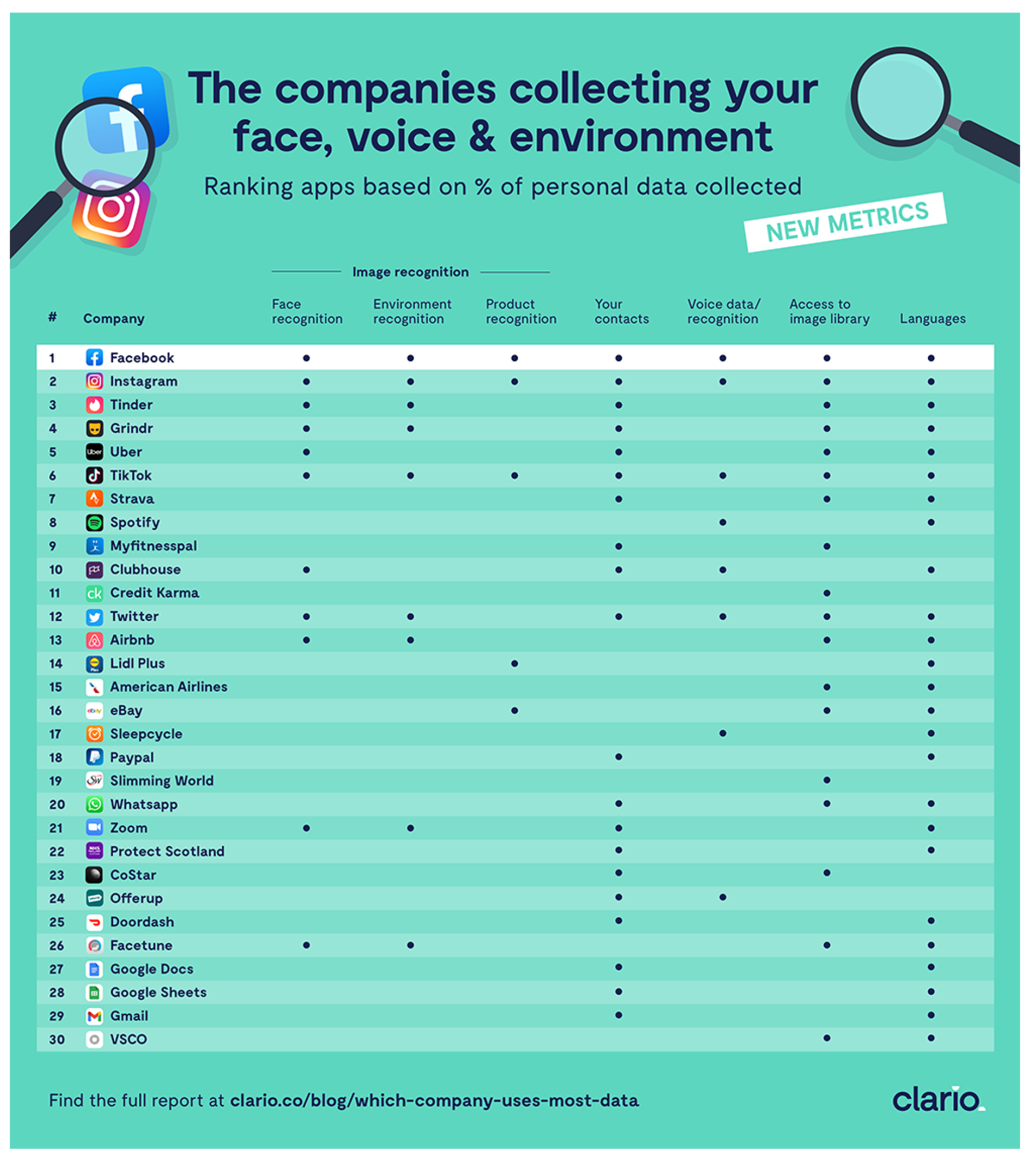
Figure 2.
Typical logistic biplot representation with probability scales. The point of the scale predicting 0.5 has been marked with a circle.
Figure 2.
Typical logistic biplot representation with probability scales. The point of the scale predicting 0.5 has been marked with a circle.
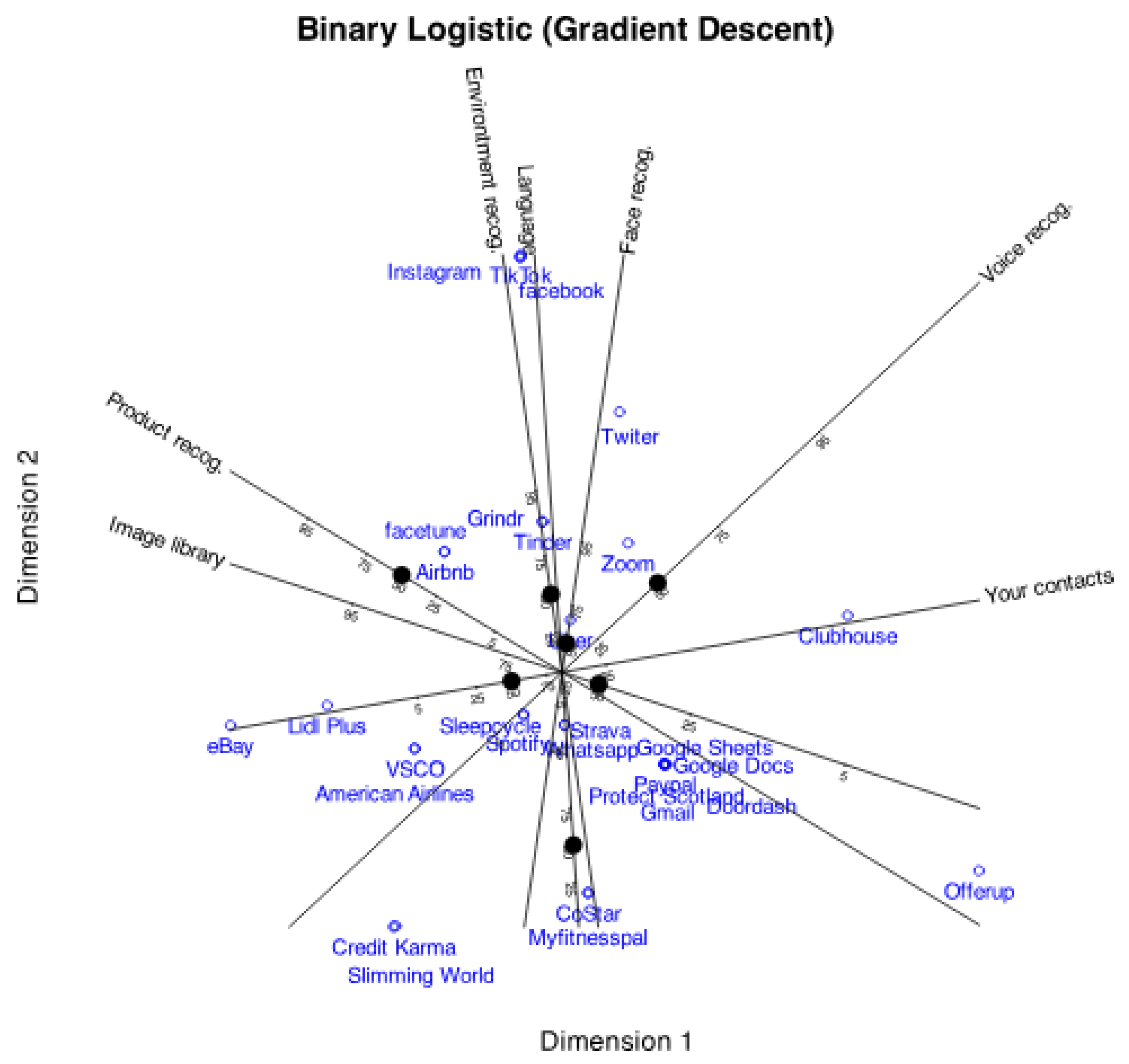
Figure 3.
Logistic biplot representation showing the projections of all the companies onto face recognition variable.
Figure 3.
Logistic biplot representation showing the projections of all the companies onto face recognition variable.
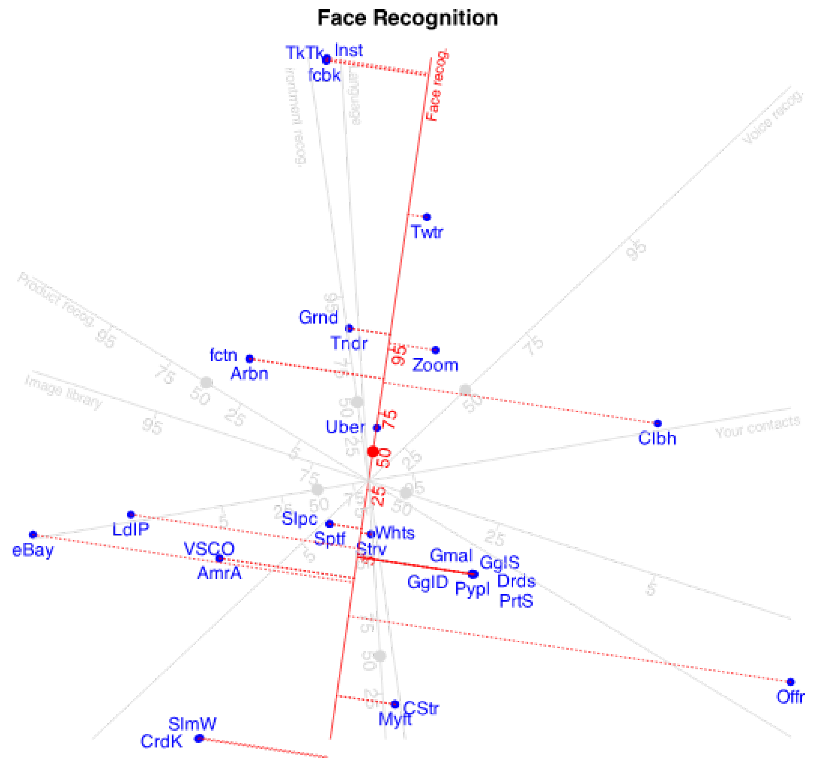
Figure 4.
Simplified logistic biplot representation with arrows starting at 0.5 and ending at 0.75 predicted probabilities.
Figure 4.
Simplified logistic biplot representation with arrows starting at 0.5 and ending at 0.75 predicted probabilities.
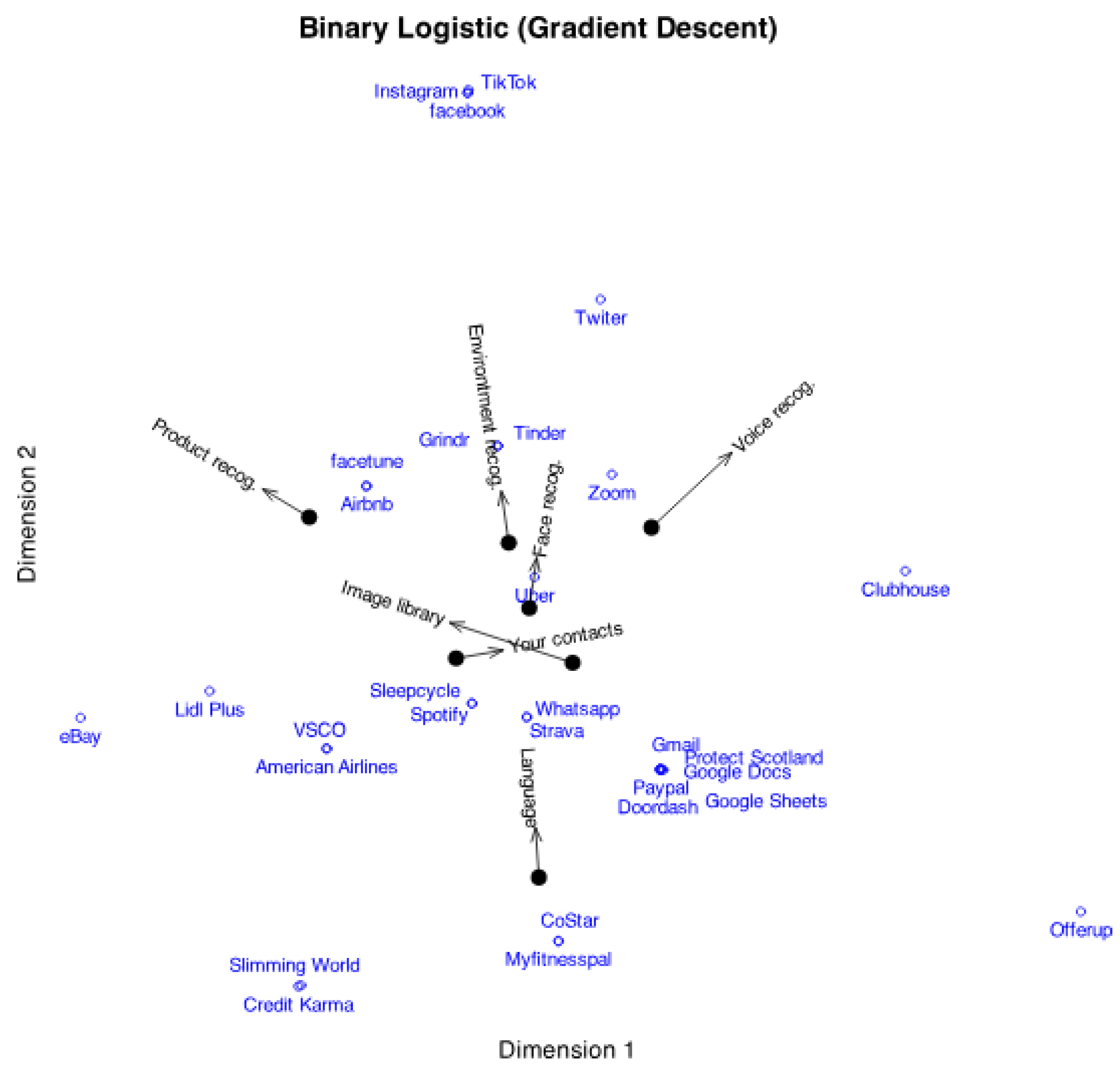
Figure 5.
Prediction regions for face recognition variable.
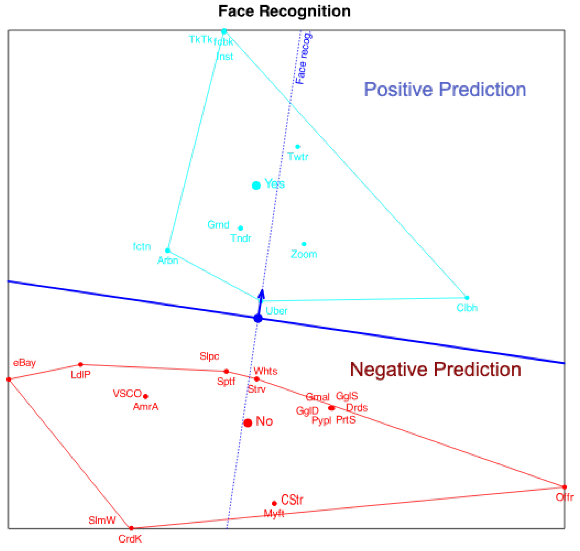
Figure 6.
Logistic biplot for the responses (countries) of the anthracnose example.
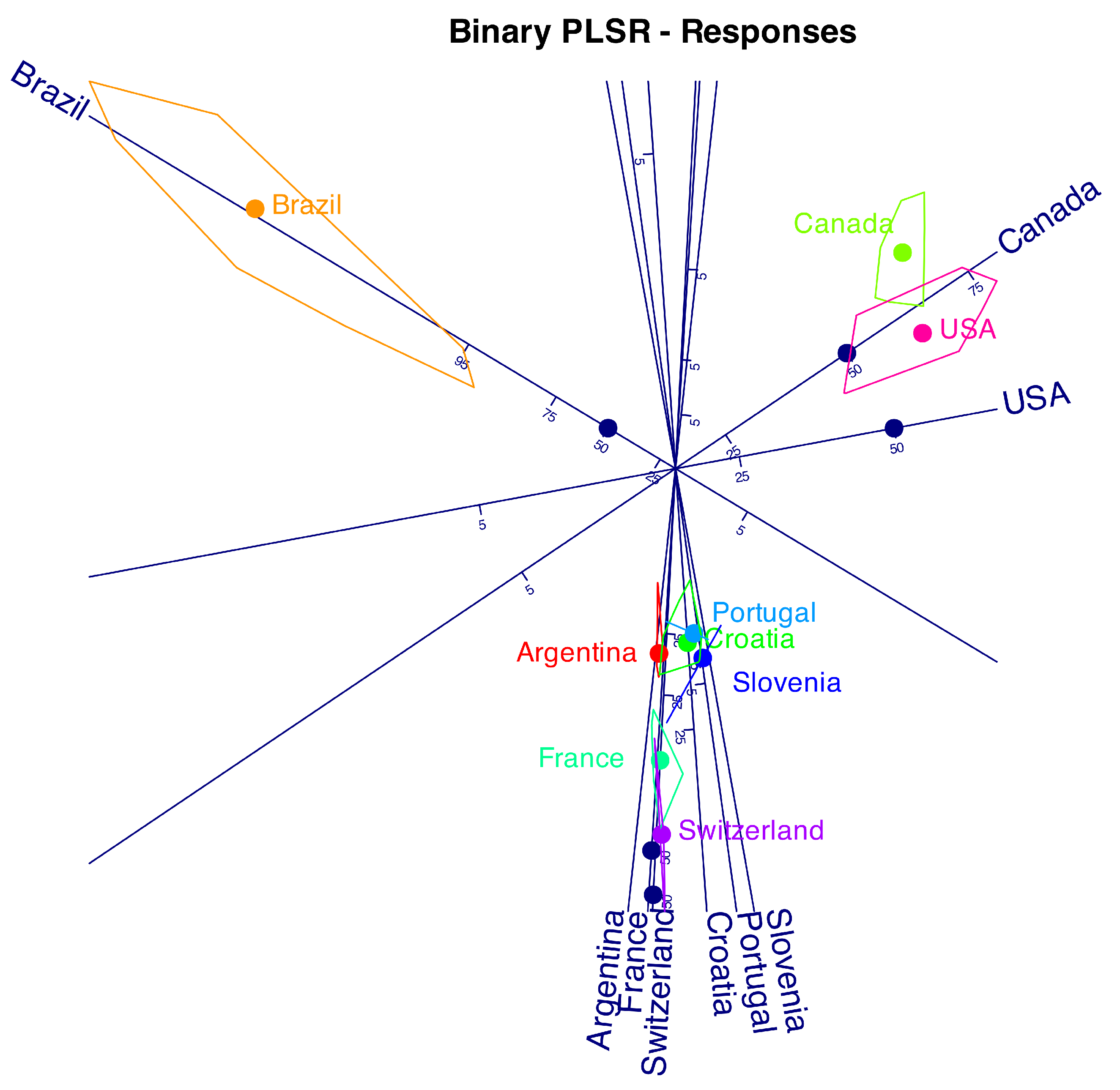
Figure 7.
Logistic biplot for the grouped responses (countries) of the anthracnose example.
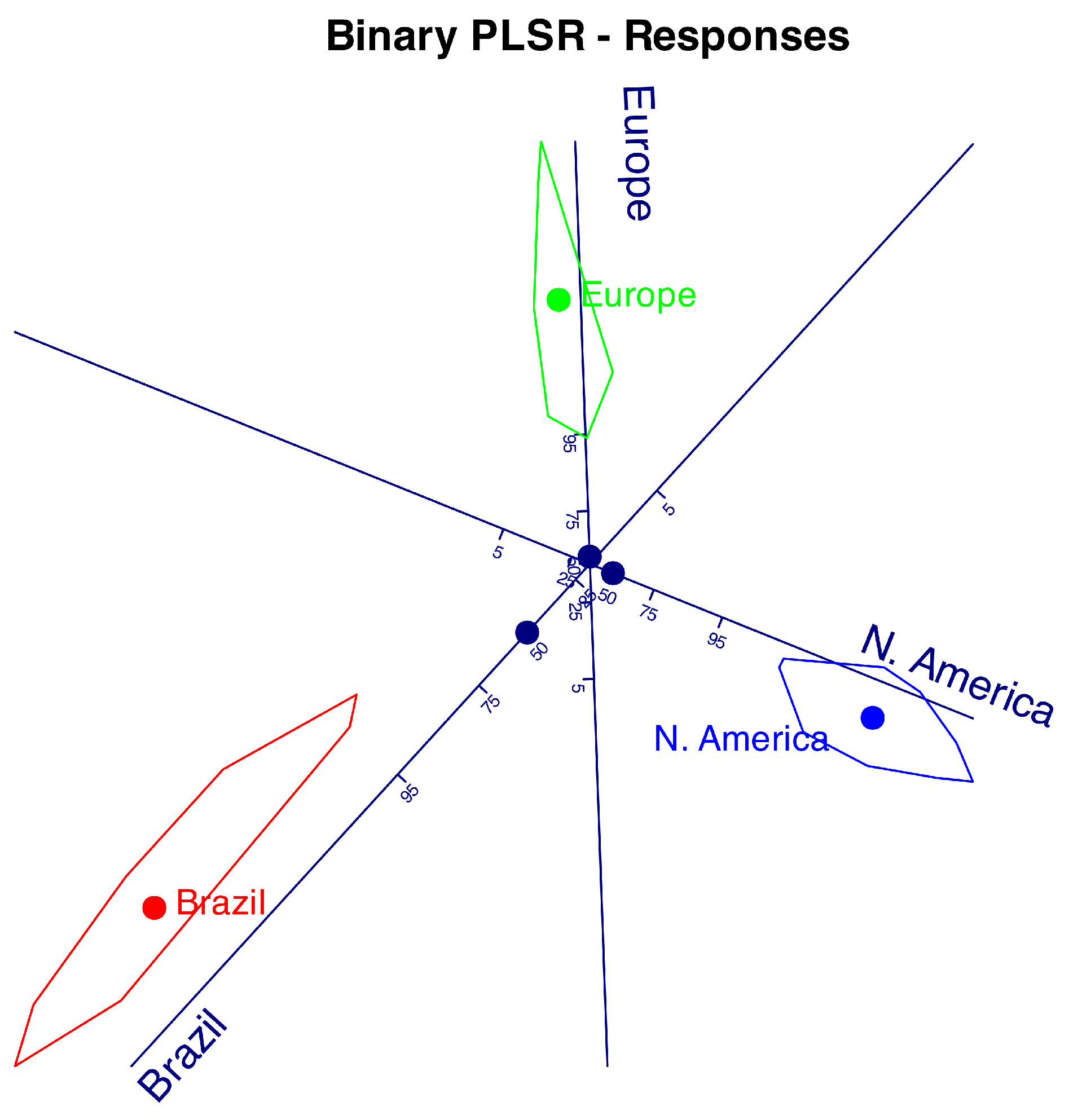
Figure 8.
Logistic triplot for the grouped countries of the anthracnose example.
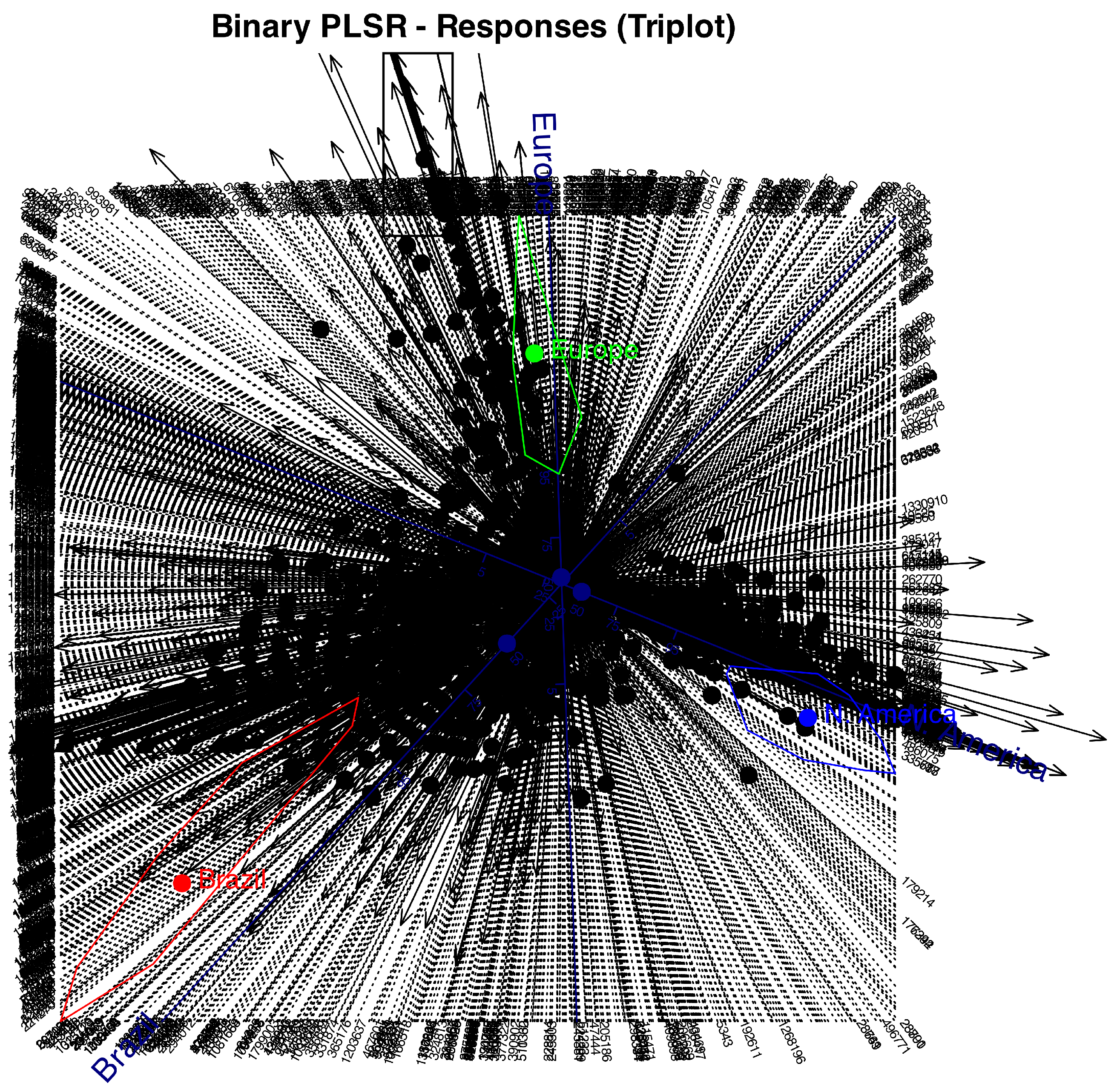
Figure 9.
Logistic triplot including the more important polimorphisms to classify Brazil
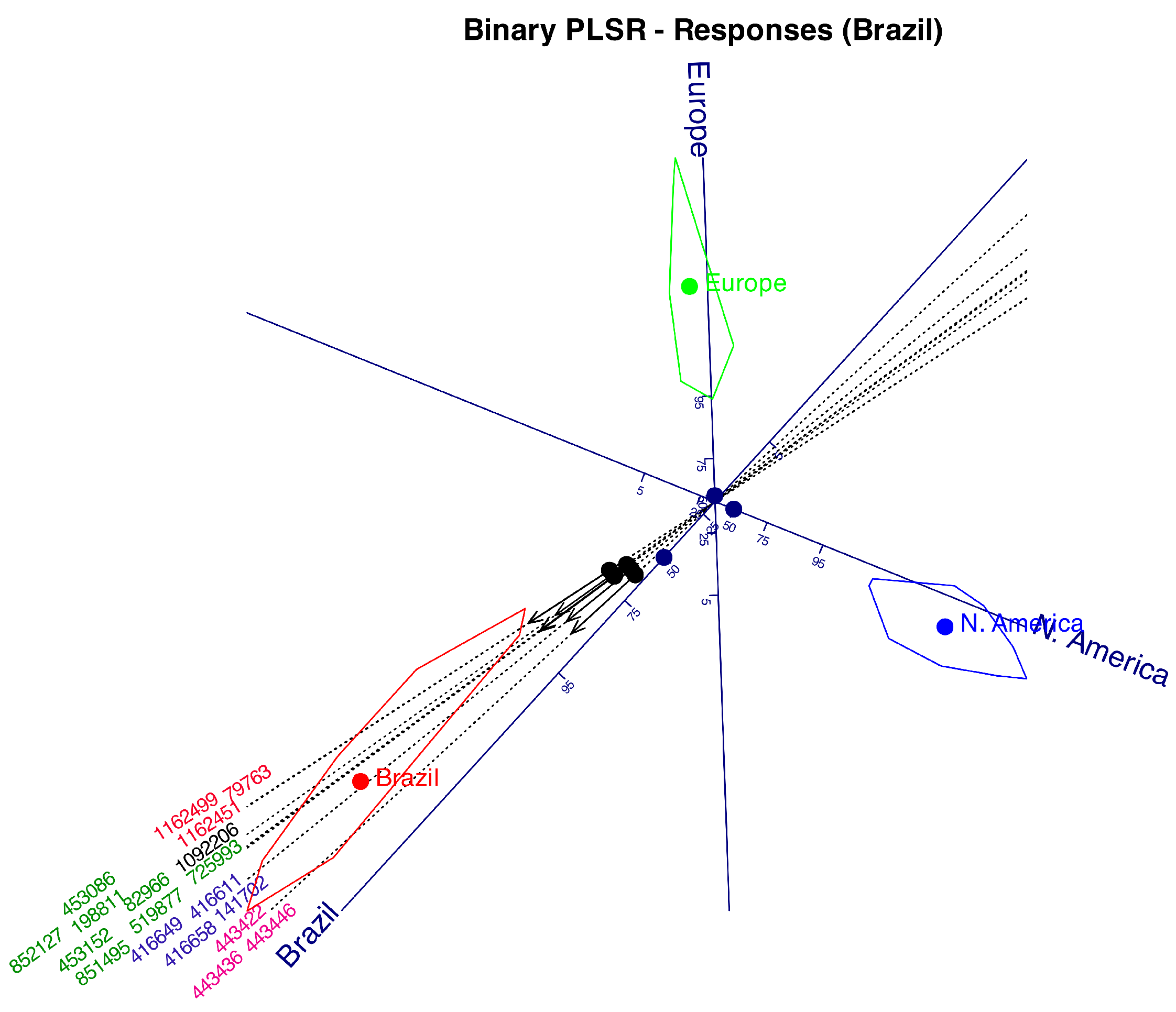
Figure 10.
Logistic triplot including the more important polimorphisms to classify Europe.
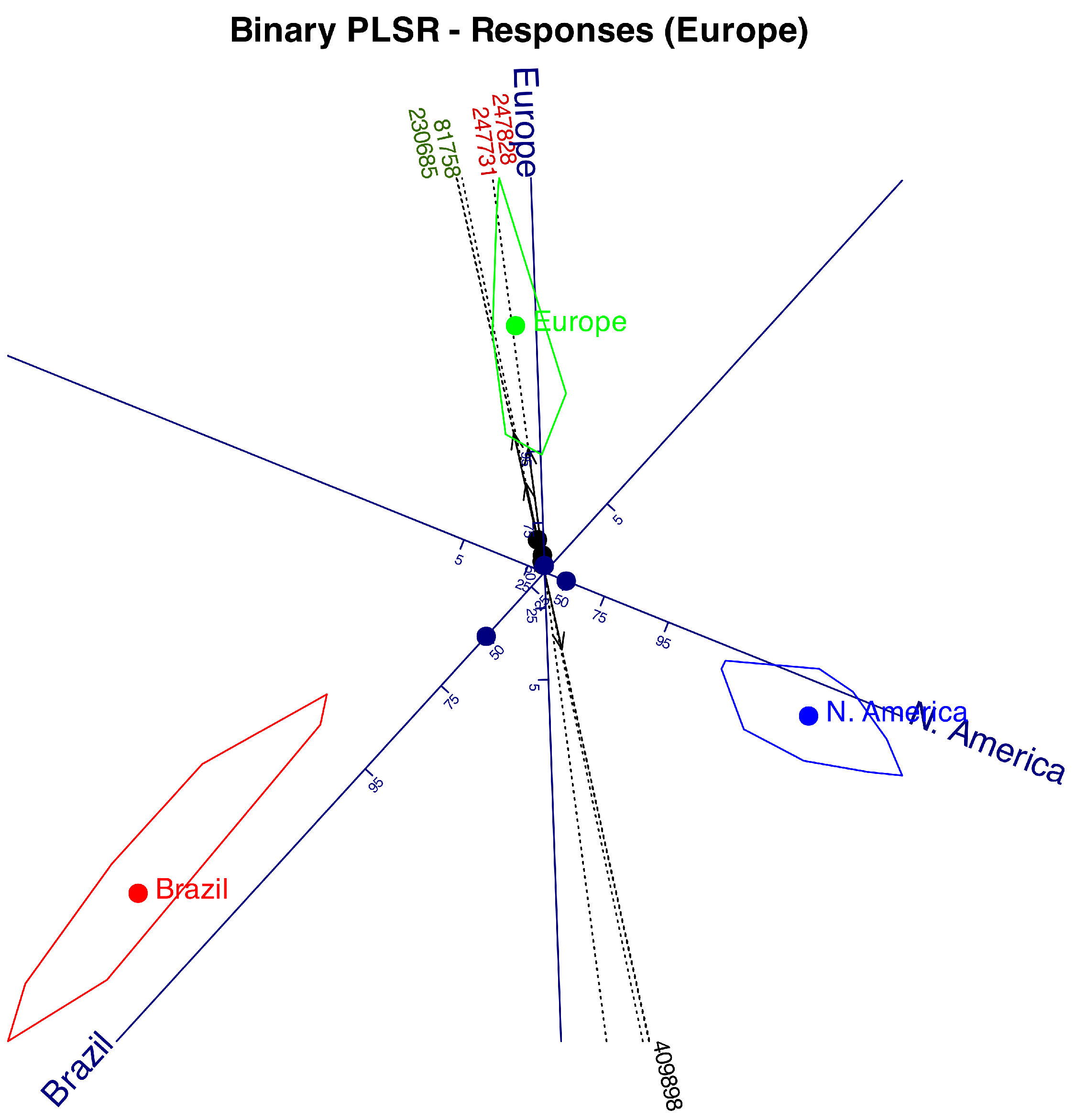
Figure 11.
Logistic triplot including the more important polimorphisms to classify North America.
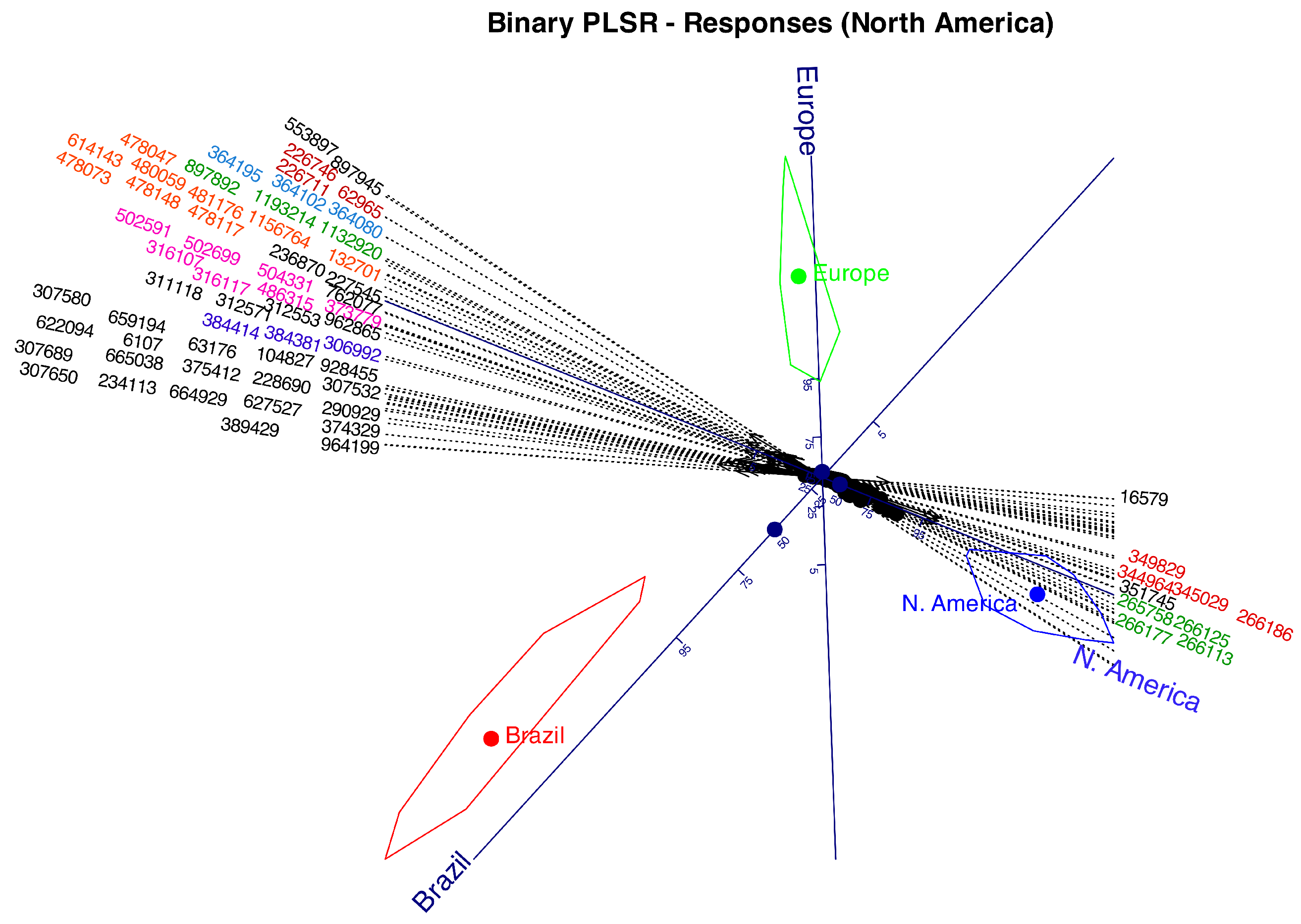

Table 1.
Internet companies.
| Company | Face rec. | Env. rec. | Prod. rec. | Contacts | Voice rec. | Image lib. | Language |
|---|---|---|---|---|---|---|---|
| 1 | 1 | 1 | 1 | 1 | 1 | 1 | |
| 1 | 1 | 1 | 1 | 1 | 1 | 1 | |
| Tinder | 1 | 1 | 0 | 1 | 0 | 1 | 1 |
| Grindr | 1 | 1 | 0 | 1 | 0 | 1 | 1 |
| Uber | 1 | 0 | 0 | 1 | 0 | 1 | 1 |
| TikTok | 1 | 1 | 1 | 1 | 1 | 1 | 1 |
| Strava | 0 | 0 | 0 | 1 | 0 | 1 | 1 |
| Spotify | 0 | 0 | 0 | 0 | 1 | 0 | 1 |
| Myfitnesspal | 0 | 0 | 0 | 1 | 0 | 1 | 0 |
| Clubhouse | 1 | 0 | 0 | 1 | 1 | 0 | 1 |
| Credit Karma | 0 | 0 | 0 | 0 | 0 | 1 | 0 |
| Twiter | 1 | 1 | 0 | 1 | 1 | 1 | 1 |
| Airbnb | 1 | 1 | 0 | 0 | 0 | 1 | 1 |
| Lidl Plus | 0 | 0 | 1 | 0 | 0 | 0 | 1 |
| American Airlines | 0 | 0 | 0 | 0 | 0 | 1 | 1 |
| eBay | 0 | 0 | 1 | 0 | 0 | 1 | 1 |
| Sleepcycle | 0 | 0 | 0 | 0 | 1 | 0 | 1 |
| Paypal | 0 | 0 | 0 | 1 | 0 | 0 | 1 |
| Slimming World | 0 | 0 | 0 | 0 | 0 | 1 | 0 |
| 0 | 0 | 0 | 1 | 0 | 1 | 1 | |
| Zoom | 1 | 1 | 0 | 1 | 0 | 0 | 1 |
| Protect Scotland | 0 | 0 | 0 | 1 | 0 | 0 | 1 |
| CoStar | 0 | 0 | 0 | 1 | 0 | 1 | 0 |
| Offerup | 0 | 0 | 0 | 1 | 1 | 0 | 0 |
| Doordash | 0 | 0 | 0 | 1 | 0 | 0 | 1 |
| Facetune | 1 | 1 | 0 | 0 | 0 | 1 | 1 |
| Google Docs | 0 | 0 | 0 | 1 | 0 | 0 | 1 |
| Google Sheets | 0 | 0 | 0 | 1 | 0 | 0 | 1 |
| Gmail | 0 | 0 | 0 | 1 | 0 | 0 | 1 |
| VSCO | 0 | 0 | 0 | 0 | 0 | 1 | 1 |
Table 2.
Measures of fit for columns.
| Deviance | D.F | P-val | Nagelkerke | Cox-Snell | MacFaden | % Correct | Sensitivity | Specificity | |
|---|---|---|---|---|---|---|---|---|---|
| Face recog. | 36.60 | 2.00 | 0.00 | 0.96 | 0.70 | 0.91 | 100.00 | 100.00 | 100.00 |
| Environtment recog. | 42.47 | 2.00 | 0.00 | 0.96 | 0.76 | 0.92 | 100.00 | 100.00 | 100.00 |
| Product recog. | 45.91 | 2.00 | 0.00 | 0.96 | 0.78 | 0.90 | 96.67 | 80.00 | 100.00 |
| Your contacts | 35.03 | 2.00 | 0.00 | 0.91 | 0.69 | 0.82 | 93.33 | 100.00 | 80.00 |
| Voice recog. | 16.98 | 2.00 | 0.00 | 0.61 | 0.43 | 0.45 | 90.00 | 75.00 | 95.45 |
| Image library | 12.69 | 2.00 | 0.00 | 0.47 | 0.34 | 0.31 | 80.00 | 88.89 | 66.67 |
| Language | 47.98 | 2.00 | 0.00 | 0.97 | 0.80 | 0.93 | 100.00 | 100.00 | 100.00 |
| Total | 237.65 | 14.00 | 0.00 | 0.88 | 0.68 | 0.77 | 94.29 | 94.79 | 93.86 |
Table 3.
Thresholds, Loadings and Communalities.
| Thresholds | Loadings | Communalities | ||
|---|---|---|---|---|
| Dim1 | Dim2 | |||
| Face recog. | -0.02 | 0.14 | 0.96 | 0.94 |
| Environtment recog. | -0.05 | -0.14 | 0.96 | 0.94 |
| Product recog. | -0.11 | -0.83 | 0.50 | 0.93 |
| Your contacts | 0.04 | 0.96 | 0.17 | 0.95 |
| Voice recog. | -0.10 | 0.64 | 0.60 | 0.77 |
| Image library | 0.03 | -0.80 | 0.26 | 0.71 |
| Language | 0.11 | -0.06 | 0.97 | 0.94 |
Table 4.
Columns Fit measures.
| Deviance | D.F | P-val | Nagelkerke | Cox-Snell | MacFaden | % Correct | Sensitivity | Specificity | |
|---|---|---|---|---|---|---|---|---|---|
| Argentina | 3.60 | 2.00 | 0.17 | 0.10 | 0.03 | 0.08 | 94.17 | 0.00 | 100.00 |
| Brazil | 95.40 | 2.00 | 0.00 | 0.96 | 0.60 | 0.94 | 100.00 | 100.00 | 100.00 |
| Canada | 35.30 | 2.00 | 0.00 | 0.48 | 0.29 | 0.37 | 85.44 | 100.00 | 82.35 |
| Croatia | 7.48 | 2.00 | 0.02 | 0.13 | 0.07 | 0.10 | 87.38 | 0.00 | 100.00 |
| France | 20.36 | 2.00 | 0.00 | 0.34 | 0.18 | 0.26 | 85.44 | 0.00 | 97.78 |
| Portugal | 1.37 | 2.00 | 0.50 | 0.06 | 0.01 | 0.05 | 97.09 | 0.00 | 100.00 |
| Slovenia | 1.81 | 2.00 | 0.41 | 0.08 | 0.02 | 0.07 | 97.09 | 0.00 | 100.00 |
| Switzerland | 19.89 | 2.00 | 0.00 | 0.39 | 0.18 | 0.33 | 93.20 | 22.22 | 100.00 |
| USA | 30.31 | 2.00 | 0.00 | 0.42 | 0.25 | 0.32 | 77.67 | 72.22 | 78.82 |
| Total | 215.52 | 18.00 | 0.00 | 0.43 | 0.21 | 0.35 | 90.83 | 51.46 | 95.75 |
Table 5.
Classification of the Countries.
| Brazil | Canada | France | |
|---|---|---|---|
| Argentina | 0 | 0 | 6 |
| Brazil | 20 | 0 | 0 |
| Canada | 0 | 18 | 0 |
| Croatia | 0 | 0 | 13 |
| France | 0 | 0 | 13 |
| Portugal | 0 | 0 | 3 |
| Slovenia | 0 | 0 | 3 |
| Switzerland | 0 | 0 | 9 |
| USA | 0 | 18 | 0 |
Table 6.
Columns Fit measures for responses of grouped data.
| Deviance | D.F | P-val | Nagelkerke | Cox-Snell | MacFaden | % Correct | Sensitivity | Specificity | |
|---|---|---|---|---|---|---|---|---|---|
| Brazil | 93.55 | 2.00 | 0.00 | 0.95 | 0.60 | 0.92 | 100.00 | 100.00 | 100.00 |
| Europe | 139.67 | 2.00 | 0.00 | 0.99 | 0.74 | 0.98 | 100.00 | 100.00 | 100.00 |
| N. America | 129.56 | 2.00 | 0.00 | 0.99 | 0.72 | 0.97 | 100.00 | 100.00 | 100.00 |
| Total | 362.78 | 6.00 | 0.00 | 0.98 | 0.69 | 0.96 | 100.00 | 100.00 | 100.00 |
Table 7.
Thresholds, Loadings and Communalities.
| Thresholds | Dim1 | Dim2 | Communalities | |
|---|---|---|---|---|
| Brazil | -0.02 | -0.65 | -0.72 | 0.94 |
| Europe | 0.00 | -0.03 | 0.99 | 0.98 |
| N. America | 0.00 | 0.92 | -0.37 | 0.98 |
Table 8.
Fit measures of the variables most related to Brazil.
| Deviance | D.F | P-val | Nagelkerke | Cox-Snell | MacFaden | % Correct | Sensitivity | Specificity | |
|---|---|---|---|---|---|---|---|---|---|
| 725993 | 79.24 | 2.00 | 0.00 | 0.87 | 0.54 | 0.80 | 99.03 | 100.00 | 98.81 |
| 851495 | 78.00 | 2.00 | 0.00 | 0.86 | 0.53 | 0.79 | 99.03 | 100.00 | 98.81 |
| 852127 | 78.00 | 2.00 | 0.00 | 0.86 | 0.53 | 0.79 | 99.03 | 100.00 | 98.81 |
| 1162451 | 79.95 | 2.00 | 0.00 | 0.86 | 0.54 | 0.79 | 98.06 | 95.00 | 98.80 |
| 1162499 | 79.95 | 2.00 | 0.00 | 0.86 | 0.54 | 0.79 | 98.06 | 95.00 | 98.80 |
| 1092206 | 87.65 | 2.00 | 0.00 | 0.90 | 0.57 | 0.84 | 99.03 | 95.24 | 100.00 |
| 453086 | 83.11 | 2.00 | 0.00 | 0.90 | 0.55 | 0.84 | 99.03 | 100.00 | 98.81 |
| 453152 | 83.11 | 2.00 | 0.00 | 0.90 | 0.55 | 0.84 | 99.03 | 100.00 | 98.81 |
| 198811 | 80.72 | 2.00 | 0.00 | 0.88 | 0.54 | 0.82 | 99.03 | 100.00 | 98.81 |
| 519877 | 83.11 | 2.00 | 0.00 | 0.90 | 0.55 | 0.84 | 99.03 | 100.00 | 98.81 |
| 416611 | 90.04 | 2.00 | 0.00 | 0.93 | 0.58 | 0.89 | 100.00 | 100.00 | 100.00 |
| 416649 | 90.04 | 2.00 | 0.00 | 0.93 | 0.58 | 0.89 | 100.00 | 100.00 | 100.00 |
| 416658 | 90.04 | 2.00 | 0.00 | 0.93 | 0.58 | 0.89 | 100.00 | 100.00 | 100.00 |
| 443422 | 85.55 | 2.00 | 0.00 | 0.89 | 0.56 | 0.82 | 99.03 | 95.24 | 100.00 |
| 443436 | 85.55 | 2.00 | 0.00 | 0.89 | 0.56 | 0.82 | 99.03 | 95.24 | 100.00 |
| 443446 | 85.55 | 2.00 | 0.00 | 0.89 | 0.56 | 0.82 | 99.03 | 95.24 | 100.00 |
| 141702 | 90.04 | 2.00 | 0.00 | 0.93 | 0.58 | 0.89 | 100.00 | 100.00 | 100.00 |
| 82966 | 83.59 | 2.00 | 0.00 | 0.90 | 0.56 | 0.85 | 99.03 | 100.00 | 98.81 |
| 79763 | 80.21 | 2.00 | 0.00 | 0.86 | 0.54 | 0.79 | 98.06 | 95.00 | 98.80 |
Table 9.
Fit measures of the variables most related to Europe.
| Deviance | D.F | P-val | Nagelkerke | Cox-Snell | MacFaden | % Correct | Sensitivity | Specificity | |
|---|---|---|---|---|---|---|---|---|---|
| 247731 | 87.77 | 2.00 | 0.00 | 0.77 | 0.57 | 0.62 | 92.23 | 91.49 | 92.86 |
| 247828 | 87.77 | 2.00 | 0.00 | 0.77 | 0.57 | 0.62 | 92.23 | 91.49 | 92.86 |
| 409898 | 112.74 | 2.00 | 0.00 | 0.89 | 0.67 | 0.79 | 95.15 | 96.36 | 93.75 |
| 81758 | 85.96 | 2.00 | 0.00 | 0.76 | 0.57 | 0.61 | 92.23 | 95.35 | 90.00 |
| 230685 | 112.20 | 2.00 | 0.00 | 0.89 | 0.66 | 0.79 | 96.12 | 93.88 | 98.15 |
Table 10.
Fit measures of the variables most related to North America.
| Deviance | D.F | P-val | Nagelkerke | Cox-Snell | MacFaden | % Correct | Sensitivity | Specificity | |
| 132701 | 81.10 | 2.00 | 0.00 | 0.73 | 0.54 | 0.57 | 89.32 | 98.28 | 77.78 |
| 1132920 | 82.01 | 2.00 | 0.00 | 0.78 | 0.55 | 0.66 | 94.17 | 91.78 | 100.00 |
| 1156764 | 71.05 | 2.00 | 0.00 | 0.72 | 0.50 | 0.59 | 92.23 | 89.33 | 100.00 |
| 1193214 | 76.35 | 2.00 | 0.00 | 0.75 | 0.52 | 0.62 | 93.20 | 90.54 | 100.00 |
| 373779 | 68.57 | 2.00 | 0.00 | 0.65 | 0.49 | 0.48 | 85.44 | 98.15 | 71.43 |
| 897892 | 94.50 | 2.00 | 0.00 | 0.81 | 0.60 | 0.67 | 92.23 | 100.00 | 81.82 |
| 897945 | 86.08 | 2.00 | 0.00 | 0.77 | 0.57 | 0.63 | 93.20 | 96.88 | 87.18 |
| 962865 | 72.23 | 2.00 | 0.00 | 0.69 | 0.50 | 0.54 | 91.26 | 93.94 | 86.49 |
| 306992 | 90.08 | 2.00 | 0.00 | 0.79 | 0.58 | 0.65 | 93.20 | 98.39 | 85.37 |
| 762077 | 73.39 | 2.00 | 0.00 | 0.71 | 0.51 | 0.57 | 91.26 | 91.43 | 90.91 |
| 290929 | 83.85 | 2.00 | 0.00 | 0.74 | 0.56 | 0.59 | 85.44 | 98.15 | 71.43 |
| 553897 | 99.66 | 2.00 | 0.00 | 0.84 | 0.62 | 0.72 | 94.17 | 98.41 | 87.50 |
| 614143 | 78.79 | 2.00 | 0.00 | 0.71 | 0.53 | 0.55 | 86.41 | 100.00 | 72.00 |
| 928455 | 82.02 | 2.00 | 0.00 | 0.73 | 0.55 | 0.57 | 85.44 | 100.00 | 70.59 |
| 964199 | 77.15 | 2.00 | 0.00 | 0.70 | 0.53 | 0.54 | 83.50 | 95.83 | 72.73 |
| 227545 | 83.45 | 2.00 | 0.00 | 0.74 | 0.56 | 0.59 | 89.32 | 100.00 | 76.60 |
| 384381 | 87.77 | 2.00 | 0.00 | 0.77 | 0.57 | 0.62 | 89.32 | 100.00 | 76.60 |
| 384414 | 87.77 | 2.00 | 0.00 | 0.77 | 0.57 | 0.62 | 89.32 | 100.00 | 76.60 |
| 389429 | 68.86 | 2.00 | 0.00 | 0.65 | 0.49 | 0.49 | 77.67 | 91.30 | 66.67 |
| 16579 | 79.07 | 2.00 | 0.00 | 0.72 | 0.54 | 0.56 | 83.50 | 72.73 | 95.83 |
| 62965 | 77.16 | 2.00 | 0.00 | 0.72 | 0.53 | 0.57 | 90.29 | 93.85 | 84.21 |
| 236870 | 111.89 | 2.00 | 0.00 | 0.91 | 0.66 | 0.84 | 98.06 | 98.51 | 97.22 |
| 307532 | 76.90 | 2.00 | 0.00 | 0.71 | 0.53 | 0.54 | 87.38 | 96.55 | 75.56 |
| 307580 | 76.90 | 2.00 | 0.00 | 0.71 | 0.53 | 0.54 | 87.38 | 96.55 | 75.56 |
| 307650 | 84.81 | 2.00 | 0.00 | 0.75 | 0.56 | 0.60 | 88.35 | 98.25 | 76.09 |
| 307689 | 84.81 | 2.00 | 0.00 | 0.75 | 0.56 | 0.60 | 88.35 | 98.25 | 76.09 |
| 311118 | 95.52 | 2.00 | 0.00 | 0.83 | 0.60 | 0.70 | 94.17 | 96.92 | 89.47 |
| 312553 | 95.52 | 2.00 | 0.00 | 0.83 | 0.60 | 0.70 | 94.17 | 96.92 | 89.47 |
| 312571 | 95.52 | 2.00 | 0.00 | 0.83 | 0.60 | 0.70 | 94.17 | 96.92 | 89.47 |
| 316107 | 95.52 | 2.00 | 0.00 | 0.83 | 0.60 | 0.70 | 94.17 | 96.92 | 89.47 |
| 316117 | 95.52 | 2.00 | 0.00 | 0.83 | 0.60 | 0.70 | 94.17 | 96.92 | 89.47 |
| 344964 | 84.37 | 2.00 | 0.00 | 0.77 | 0.56 | 0.63 | 92.23 | 88.89 | 94.03 |
| 345029 | 84.37 | 2.00 | 0.00 | 0.77 | 0.56 | 0.63 | 92.23 | 88.89 | 94.03 |
| 349829 | 84.37 | 2.00 | 0.00 | 0.77 | 0.56 | 0.63 | 92.23 | 88.89 | 94.03 |
| 351745 | 87.15 | 2.00 | 0.00 | 0.79 | 0.57 | 0.66 | 93.20 | 91.43 | 94.12 |
| 486315 | 71.90 | 2.00 | 0.00 | 0.70 | 0.50 | 0.54 | 91.26 | 92.65 | 88.57 |
| 622094 | 75.72 | 2.00 | 0.00 | 0.70 | 0.52 | 0.54 | 87.38 | 96.55 | 75.56 |
| 627527 | 77.08 | 2.00 | 0.00 | 0.71 | 0.53 | 0.55 | 87.38 | 96.55 | 75.56 |
| 659194 | 78.95 | 2.00 | 0.00 | 0.72 | 0.54 | 0.56 | 88.35 | 96.61 | 77.27 |
| 664929 | 73.80 | 2.00 | 0.00 | 0.68 | 0.51 | 0.52 | 86.41 | 96.49 | 73.91 |
| 665038 | 73.80 | 2.00 | 0.00 | 0.68 | 0.51 | 0.52 | 86.41 | 96.49 | 73.91 |
| 502591 | 71.17 | 2.00 | 0.00 | 0.67 | 0.50 | 0.51 | 89.32 | 96.67 | 79.07 |
| 502699 | 71.17 | 2.00 | 0.00 | 0.67 | 0.50 | 0.51 | 89.32 | 96.67 | 79.07 |
| 504331 | 71.17 | 2.00 | 0.00 | 0.67 | 0.50 | 0.51 | 89.32 | 96.67 | 79.07 |
| 226711 | 70.15 | 2.00 | 0.00 | 0.66 | 0.49 | 0.49 | 86.41 | 100.00 | 72.00 |
| 226746 | 70.15 | 2.00 | 0.00 | 0.66 | 0.49 | 0.49 | 86.41 | 100.00 | 72.00 |
| 228690 | 62.55 | 2.00 | 0.00 | 0.61 | 0.46 | 0.44 | 83.50 | 100.00 | 67.92 |
| 478047 | 85.07 | 2.00 | 0.00 | 0.79 | 0.56 | 0.66 | 95.15 | 94.29 | 96.97 |
| 478073 | 85.07 | 2.00 | 0.00 | 0.79 | 0.56 | 0.66 | 95.15 | 94.29 | 96.97 |
| 478117 | 85.07 | 2.00 | 0.00 | 0.79 | 0.56 | 0.66 | 95.15 | 94.29 | 96.97 |
| 478148 | 85.07 | 2.00 | 0.00 | 0.79 | 0.56 | 0.66 | 95.15 | 94.29 | 96.97 |
| 480059 | 85.07 | 2.00 | 0.00 | 0.79 | 0.56 | 0.66 | 95.15 | 94.29 | 96.97 |
| 481176 | 85.07 | 2.00 | 0.00 | 0.79 | 0.56 | 0.66 | 95.15 | 94.29 | 96.97 |
| 234113 | 77.47 | 2.00 | 0.00 | 0.71 | 0.53 | 0.54 | 86.41 | 98.18 | 72.92 |
| 364080 | 81.82 | 2.00 | 0.00 | 0.74 | 0.55 | 0.59 | 91.26 | 96.77 | 82.93 |
| 364102 | 81.82 | 2.00 | 0.00 | 0.74 | 0.55 | 0.59 | 91.26 | 96.77 | 82.93 |
| 364195 | 81.82 | 2.00 | 0.00 | 0.74 | 0.55 | 0.59 | 91.26 | 96.77 | 82.93 |
| 374329 | 82.47 | 2.00 | 0.00 | 0.73 | 0.55 | 0.58 | 79.61 | 92.00 | 67.92 |
| 375412 | 75.50 | 2.00 | 0.00 | 0.70 | 0.52 | 0.53 | 87.38 | 96.55 | 75.56 |
| 265758 | 88.81 | 2.00 | 0.00 | 0.80 | 0.58 | 0.68 | 94.17 | 94.12 | 94.20 |
| 266113 | 88.81 | 2.00 | 0.00 | 0.80 | 0.58 | 0.68 | 94.17 | 94.12 | 94.20 |
| 266125 | 88.81 | 2.00 | 0.00 | 0.80 | 0.58 | 0.68 | 94.17 | 94.12 | 94.20 |
| 266177 | 88.81 | 2.00 | 0.00 | 0.80 | 0.58 | 0.68 | 94.17 | 94.12 | 94.20 |
| 266186 | 88.81 | 2.00 | 0.00 | 0.80 | 0.58 | 0.68 | 94.17 | 94.12 | 94.20 |
| 6107 | 78.86 | 2.00 | 0.00 | 0.72 | 0.53 | 0.56 | 87.38 | 98.21 | 74.47 |
| 104827 | 67.60 | 2.00 | 0.00 | 0.64 | 0.48 | 0.48 | 83.50 | 100.00 | 69.09 |
Disclaimer/Publisher’s Note: The statements, opinions and data contained in all publications are solely those of the individual author(s) and contributor(s) and not of MDPI and/or the editor(s). MDPI and/or the editor(s) disclaim responsibility for any injury to people or property resulting from any ideas, methods, instructions or products referred to in the content. |
© 2024 by the authors. Licensee MDPI, Basel, Switzerland. This article is an open access article distributed under the terms and conditions of the Creative Commons Attribution (CC BY) license (http://creativecommons.org/licenses/by/4.0/).
Copyright: This open access article is published under a Creative Commons CC BY 4.0 license, which permit the free download, distribution, and reuse, provided that the author and preprint are cited in any reuse.


