Submitted:
21 May 2025
Posted:
27 May 2025
You are already at the latest version
Abstract
We present a thorough machine-learning framework based on real-time state of polarization (SOP) monitoring for robust anomaly identification in optical fiber networks. We exploit SOP data under three different threat scenarios: (i) malicious or critical vibration events, (ii) overlapping mechanical disturbances, and (iii) malicious fiber tapping (eavesdropping). We have used various supervised machine learning techniques like k-Nearest Neighbor (kNN), random forest, extreme gradient boosting (XGBoost) and decision trees to classify different vibration events. We also assessed the framework’s resilience to background interference by superimposing sinusoidal noise at different frequencies and examining its effects on the polarization signatures. This analysis provides insight into how subsurface installations, subject to ambient vibrations, affect detection fidelity. This highlights the sensitivity to which external interference affects polarization fingerprints. Crucially, it demonstrates the system’s capacity to discern and alert on malicious vibration events even in the presence of environmental noise. However, we focus on the necessity of noise-mitigation techniques in real-world implementations while providing a potent, real-time mechanism for multi-threat recognition in the fiber networks.
Keywords:
state of polarization
; machine learning
; random forest
; XGBoost
; decision tree
; kNN
; SOPAS
; optical fiber
; eavesdropping
; multi-vibrations
; fiber anomalies
1. Introduction
Optical networks serve as the critical infrastructure for enabling ultra-high-speed and high-capacity data transmission in contemporary telecommunication systems. The exponential surge in internet traffic, emerging 6G applications, and rising demand for high-bandwidth services necessitates the optimization of optical network performance and reliability [1]. Optical communication systems transmit exceptionally large volumes of data, including confidential and sensitive information across extensive distances. As such, ensuring the integrity and reliability of data transmission is of paramount importance in maintaining secure and trustworthy communication infrastructures [2]. The use of pre-installed optical fiber infrastructures for environmental monitoring has garnered more attention in recent years due to the extensive deployment of optical fiber networks in both terrestrial and subsea scenarios [3,4,5].
Fiber-optic cables are intrinsically sensitive to environmental conditions like temperature, mechanical stress, and vibrations [6,7]. Distributed Acoustic Sensing (DAS) systems can detect dynamic events like mechanical vibrations up to the range of kHz, and are being widely used for earthquake detection [8,9] and metropolitan monitoring [10,11]. As we know, optical fiber networks form the backbone of global connectivity, linking billions of users worldwide. Their indispensable function and inherent sensitivity, however, render them susceptible to a range of impairments—including fiber breaks, targeted physical tampering, unauthorized eavesdropping via fiber bending, and ambient mechanical vibrations [12,13]. Such perturbations can degrade the propagating optical signal, leading to severe network impairments, widespread service outages, data corruption or loss, and breaches of data confidentiality. To provide early warnings for situations that endanger the health of optical fiber networks, monitoring the metropolitan environment is very essential. Thus, it is crucial to classify and localize the fiber anomalies and limit their impact by taking proactive measures. Numerous studies have addressed the classification and localization of fiber anomalies; for instance, [14] utilized optical time-domain reflectometry (OTDR) trace analysis to detect and pinpoint disruptive events. In contrast, monitoring the state of polarization (SOP) offers greater sensitivity to subtle physical perturbations, as it directly captures alterations in the polarization state of light propagating through the fiber and can discriminate the type of anomaly. The study in [15] employs the angular speed of SOP (SOPAS) compared against a predetermined threshold to identify fiber impairments such as bending, shaking, or minor impact and other external disturbances. Meanwhile, the authors of [16] use transfer learning on SOP-derived data, transforming polarization measurements into visual formats to classify threat events.
Despite these advances, a cohesive and resilient framework for real-time SOP-based multi-threat detection remains underexplored. Machine learning (ML) models offer a powerful solution by learning complex patterns in high-dimensional SOP data. In order to identify and locate fiber problems in optical networks, recent research has used both supervised and unsupervised deep learning. An autoencoder is employed to detect anomalies in optical fibers, followed by an attention-based bidirectional gated recurrent unit (BiGRU) architecture to classify and accurately localize the events [14]. Multi-task long short term memory (LSTM) models on OTDR traces have been used to address reflective faults (such as damaged connectors or splices), providing precise detection and location even at low signal to noise ratio (SNR) [17]. The work in [18] uses the data clustering module (DCM) to analyze the patterns of the monitoring data and the convolutional autoencoder to extract features and clustering to locate the location.
Our study proposes a machine learning-based framework that takes advantage of the angular speed and temporal evolution of SOP (SOPAS) to detect and classify multiple fiber anomalies, including malicious vibrations, overlapping physical disturbances, and fiber tapping events. We evaluate the robustness of this model by introducing synthetic noise to emulate real-world environmental interference and assess the classifier’s ability to distinguish between benign and malicious anomalies. Our key objective is to create a lightweight yet resilient SOP-based monitoring architecture that can trigger alerts or initiate rerouting protocols based on the severity of the detected anomaly, thus improving the self-healing and defensive capabilities of optical networks. This work builds upon and extends our previous contributions in the field [19,20,21], aiming to bridge the gap between experimental SOP monitoring and deployable anomaly detection systems.
2. State of Polarization (SOP) as a Sensing Mechanism
The SOP serves as a highly sensitive, real-time sensing mechanism for detecting mechanical disturbances in optical fiber networks. The direction of the electric field as it moves through the fiber is known as the polarization state. Optical fiber sensors exhibit polarization sensitivity and are typically prone to polarization fading [22]. Monitoring the polarization state trajectory on the Poincaré sphere allows SOP analysis to detect minute birefringence shifts caused by temperature changes, traffic and external mechanical disturbances (e.g., drilling vibrations). In laboratory experiments, polarimeters coupled with programmable vibration sources (typically 1–10 Hz) provide high-fidelity measurement of the stokes parameters. Each SOP recording is composed of multiple variables, incorporating the variation of stokes parameters over time [23]. Variations in SOP could indicate fiber anomalies. Early detection of fiber damage or anomalies is made possible by monitoring these fluctuations. There are four stoke parameters (, , , and ) which characterize the polarization state of electromagnetic waves, or light. represents the total intensity or power of the optical beam or light while the other three components, , , and , are coordinate values in the coordinate system that a Poincaré sphere represents. is the difference in intensity between horizontally and vertically polarized light. is the difference in intensity between the diagonal () and anti-diagonal (). And represents the difference in intensity between left and right circular polarized components [24]. Any perfect polarization can be expressed as a point on the Poincaré sphere [5].
The time variation of the stokes parameters’ speed on the Poincar’e sphere at a specific angle is defined by SOPAS [25]. The formula is given by
where the sample period is denoted by . The dot product of the stokes vectors at time k and time is represented by , which indicates the extent to which these two vectors point in the same direction. The magnitude of the two stokes vectors is represented by the denominator.
To quantify the rate of change of the polarization orientation between successive stokes vectors and throughout the sampling period , the SOP angular speed, represented by the symbol , uses units of . The ratio of polarized to total light intensity in the fiber is known as the degree of polarization (DOP), and it is always 1. The strength of vibration is correlated with the SOPAS.
Polarization controllers are used to establish a desired polarization state in polarization-managed sensing networks. Standard optical fibers, on the other hand, cannot maintain this condition, leading to unexpected polarization at any point along the fiber instead of user-defined values [26]. However, SOP measurements in real-world installations have to deal with noise sources such as scattered ambient light, normalization problems in telemetry interfaces.
In this paper, we investigate the use of optical fiber as a sensing medium and present three distinct scenarios involving anomaly detection through the analysis of the SOP data obtained from a polarimeter. Machine learning techniques are employed to classify these anomalies, which may indicate potential threats to network integrity. The identified scenarios are detailed in Sections III, IV, and V. Section VI outlines the machine learning architecture implemented for vibration detection. In Section VII, we evaluate the model’s performance under varying vibration intensities and in the presence of additive noise, followed by a comparative analysis. The study concludes with key findings summarized in Section VIII.
3. Eavesdropping
An adversary, known as a hacker, could compromise the physical layer of the telecommunications system to intercept private information and harm vendors. Fiber tapping is the most popular of the various fiber-tampering techniques that have been identified [27]. It involves macro-bending the fiber cable at a low curvature radius to compromise the total internal reflection condition that permits light propagation. Light then leaks from the fiber at the bending point, where it can be intercepted by an eavesdropping device. The communication system may experience a small power reduction received [28,29] as well as a bending-induced SOP change [30], both of which a SOP detection system can identify.
To simulate such an occurrence, we used a commercial optical fiber identification (OFI) tool that clamps and heavily bends the fiber connected between a 13 Km of metropolitan fiber [31]. A handgrip that is tightened to bend the fiber inside the instrument controls the clamping. Eavesdropping occurs when the device senses light leakage. Additionally, it indicates the direction of the light leak, making it simple for a hacker to retrieve the data from the leaking light.
The behavior of the four stokes parameters for the same repeated experiments is shown in Figure 1. It illustrates how bending has an adverse impact on the stoke parameters. Initial experiments were conducted with OFI securely fastened to the optical bench, separating it from outside influences, in order to describe the signature that the macro-bends had on the SOP. After being gently clamped for 30 seconds, the fiber was released. The component records the instantaneous power, and the polarimeter outputs the whole stokes vector. The results of six tests are shown in Figure 1, where all the behavior of the stoke parameters can be observed for a clamp held for approximately 10 seconds. The instantaneous power gradually changes between levels over a period of about 1 second when the clamp is closed, and show a sudden spike, respectively. The eavesdropping tests were repeated approximately 50 times to provide a more thorough understanding of the stoke parameters’ response.
We also computed the SOPAS deviation according to Equation. 1. The higher peaks of the angular speed mean the parts when the clamp is closed, with the highest angular speed being 2.5 radians per second. In a real-world scenario, a malicious hacker would likely manipulate the optical fiber before connecting it to the device, rather than placing it firmly on a surface. In addition, the device would typically remain attached to the cable for several hours to maximize data intercept. These SOPAS and their temporal derivatives are integrated as key features for vibration event classification in our ML approach (Section VI).
4. Simultaneous Events
We also examined, how polarization signatures appear when two disruptive events occur simultaneously. Every disrupting event has a distinct polarization signature. We have generated several signatures to monitor the polarization state change on the Poincar`e sphere. These signatures have been synthesized to capture the dynamic evolution of the polarization state.
Intentional or construction-site fiber shaking, as well as tapping (eavesdropping) into the fiber to leak private and sensitive information, is considered a hostile incursion that can mislead network operators. A sophisticated ML model is needed in these situations so that it can identify and distinguish between the events and notify the service providers. Identification is made more difficult by these overlapping disturbances, which calls for more advanced detection methods [14].
In this section, we investigated the use of ML-driven SOP analysis for the detection of overlapping anomalies in optical networks. Utilizing XGBoost [32], our model accurately classified overlapping fiber anomalies, which are further discussed in [21]. The results demonstrated that for proactive network maintenance and enhanced fiber infrastructure security, ML is more accurate and dependable than traditional fault detection techniques.
For this experiment, we used a robotic arm that uses a frequency of 3 Hz and an angle of deviation to move the fiber up and down for shaking. We manually tapped the fiber once every second to hit it. Because each event generates a unique polarization signature, we captured them using the stokes parameters, as shown in Figure 2). The pronounced peaks in these traces correspond to the physical tapping (fiber hits). However, the robotic arm’s coordinated action of shaking the fiber and hitting it was synchronized for the creation of overlapping events.
Following the collection of this data, we carried a few pre-processing procedures, and then feed the dataset into our model. The results, discussed in [21] concluded that XGBoost achieved higher accuracy than the other classifiers, as it effectively captured non-linear patterns and is computationally efficient. Therefore, it was chosen for further analysis. The model accurately predicted the data with an accuracy of 98%, and only misclassified 2.06% of overlap events.
This ML model enables real-time identification of multiple threat scenarios by effectively differentiating between benign vibrations and deliberate intrusions (e.g., tapping), owing to its training on overlapping tampering events and noise-augmented datasets. It provides a robust framework for enhancing network resilience against complex and evolving fault conditions.
5. State-of-Polarization-Based Vibration Monitoring Architecture
In this section, we will describe the complete architecture of the vibration monitoring system and the experimental setup through which the dataset was collected.
In Figure 3, we can observe the different levels of shaking and their corresponding signatures as represented by the stoke parameters. As the shaking increases, the range of variation in the stokes parameters decreases. In the noise-free data shown in Figure 3, for 10 Hz shaking, the value of component oscillates between 0.25 to 0.45 whereas it spans a wider range of 0.15 to 0.65 under 3 Hz excitation.
Upon introducing varying noise levels into the dataset, the polarization signatures, corresponding to each shaking frequency exhibited noticeable shifts. For instance, Figure 4 illustrates a comparative analysis of the stokes parameter trajectories between the clean dataset and the dataset contaminated with 3 Hz noise, highlighting the distortion introduced by external perturbations. To gain a more granular understanding, each stokes parameter has been individually analyzed in the figure to clearly visualize the impact and shift caused by the 3 Hz noise. The dotted lines indicate the fingerprints affected by added noise, while the solid lines represent the original, unaltered fingerprints.
5.1. Vibration Emulation and State-of-Polarization Sensing Setup
Each event produces a distinct polarization signature. To study these, we generated multiple signatures by tracking changes in the polarization state on the Poincaré sphere using stokes parameters. We used an Arduino-controlled robotic arm to generate the shaking of various frequencies. These events are explained in Table 1, where those that do not affect the fiber’s integrity are classified as "No event". "Shaking (1Hz)" are the ones that function as ambient sound and have a lower level of severity. "Shaking (3Hz)" are moderately sensitive and it can cause mild disturbances in the metropolitan fiber. Whereas "Shaking (5Hz) and Shaking (10Hz)" are more sensitive to fiber integrity and require countermeasures. The vibration generation testbed is detailed in our earlier study [20]. A continuous-wave laser source emitting light at 1530 nm with 6 dBm power is launched into the sensing fiber. The testbed includes two segments of single-mode fiber (SMF), 8 km and 5 km in length, connected to an SMF section manipulated by the robotic arm. The Arduino-based arm is integrated into a custom printed circuit biard (PCB) along with its driver board and Arduino UNO R3 for improved stability. At the receiver end, another fiber spool is linked to a Novoptel PM1000 Polarimeter, which records the temporal evolution of stokes parameters to identify polarization signatures.
We set the sampling at 1500 samples per second. The averaging time exponent (ATE) is set to 16. The polarimeter analyzes the orientation of light scattered on the Poincaré sphere. SOPAS evaluations are generated by extrapolating the polarization state changes caused by the robotic arm. We recorded unique polarization signatures of vibrations, as outlined in the previous section, to differentiate between critical intensity levels. These experiments, done by robotic arm, generated SOP and SOPAS data reflecting each vibration level, which were then used to train and evaluate our ML model.
6. Machine Learning Model Architecture
The machine learning architecture proposed in this study is purposefully designed to detect and classify mechanical anomalies in optical fiber networks by analyzing the temporal evolution of polarization states. The input data consist of time-series measurements of the stokes parameters and corresponding angular speed, sampled at a frequency of 1500 samples per second. This fine-grained temporal resolution enables the system to capture minute polarization fluctuations indicative of vibrational disturbances or external intrusions.
To enhance the model’s ability to capture temporal dynamics, the raw polarization data are transformed into a higher-dimensional feature representation. This is achieved by incorporating temporally shifted (lagged) instances of each stokes parameter and the SOPAS up to third order, thereby enabling the model to learn from recent temporal patterns and transitional behavior. In parallel, rolling statistical descriptors, including localized means and standard deviations, are computed over sliding windows to extract trend sensitive features while attenuating transient noise and fluctuations.
Each data instance is associated with a class label corresponding to the severity of the induced mechanical disturbance: No Event, Shaking at 1 Hz, 3 Hz, 5 Hz, or 10 Hz. The dataset is partitioned into training and testing sets using a conventional 80:20 split. This structured representation enables the application of supervised learning methods capable of identifying complex patterns in both clean and noisy environments. The resulting architecture is structured to support efficient training and inference, with a moderate computational footprint and compatibility with a range of classification models. Figure 5 illustrates the complete machine learning framework, including the training process, classifier integration, and real-time event classification. The flowchart outlines key steps such as data preprocessing, feature extraction, model training, and the classification of new SOP data. After training, the classifier is used to assess the severity of unseen polarization events and generate alerts accordingly, enabling timely response to potential fiber anomalies. The subsequent section presents the supervised learning models evaluated within this framework, detailing their implementation, configuration parameters, and comparative performance.
6.1. Machine Learning Classifiers
To find the best classifier for our malicious vibrations classification task, we thoroughly examined a number of supervised machine learning techniques. We have chosen different classifiers from the Scikit-Learn package according to their performance metrics, utility, and effective predictability [33]. We employed K-nearest neighbor (kNN), decision trees, random forests (RF), and extreme gradient boosting (XGBoost) in our investigation, which are explained in detail below.
RF is a powerful supervised learning algorithm designed for both classification and regression problems. It operates by constructing an ensemble of decision trees, each trained on a randomly sampled subset of the training data through a bootstrap aggregation (bagging) process. In this study, we employed a forest consisting of 100 decision trees, each with a maximum depth limited to 6, to control model complexity and reduce the risk of overfitting. RF improves predictive performance by averaging the outputs of individual trees, which enhances generalization and mitigates variance. Additionally, it leverages dimensionality reduction and parallel computation, enabling faster training and more robust handling of high-dimensional data and noise [34].
The kNN classifier assigns unlabeled data points to the class of the most similar labeled instances based on their proximity in the feature space [35]. The labels of the K-nearest patterns in the data space serve as the foundation for nearest neighbor techniques [36]. Since it establishes how many neighbors to take into account while making predictions, the value of k is crucial in kNN. A greater k can assist in smoothing out the predictions and lessening the impact of noisy data if the dataset contains significant outliers or noise. We selected the value of K to be in range [5,50] to ensure robust classification performance across varying data distributions.
Decision trees are a supervised classification technique that uses a tree-like decision model that depends on the dataset values [37]. A decision tree solves the problem by using the tree representation, where each leaf node represents a class label and the internal nodes of the tree represent the features. The decision tree can be used to represent any Boolean function on discrete attributes. We have kept the depth of tree in our model to [3, 5, 10, 15, 20], to reduce overfitting.
XGBoost is an ensemble learning method that integrates predictions from numerous weak models for a more robust prediction. It uses a classification and regression tree (CART) as its primary learning [32]. It is also compatible with parallel processing, allowing one to train models on large datasets in a practical time frame. We have trained 150 decision trees with a learning rate of 0.4.
6.2. Evaluation Metrics
To evaluate the performance of our model, we used standard metrics derived from the confusion matrix namely: accuracy, precision, recall, and F-1-score. These metrics help quantify how well the model distinguishes between different event types, including No Event, Shaking - 1 Hz, Shaking - 3 Hz, Shaking - 5 Hz and Shaking - 10 Hz.
6.2.1. Confusion Matrix
The confusion matrix is a fundamental evaluation tool in supervised learning, offering a comprehensive breakdown of classification outcomes. It contrasts the actual class labels against the predicted ones to assess the model’s ability to distinguish between multiple event types. The confusion matrix shows a tabular representation consisting of actual and predicted class labels, shown in Table 2. Here, True Positives (TP) and True Negatives (TN) represent instances correctly classified as belonging or not belonging to a particular class, respectively. False Positives (FP) correspond to instances incorrectly assigned to a class, while False Negatives (FN) denote those that were wrongly excluded.
In our multi-class classification scenarios—where the classes represent discrete vibration levels including “No Event”, “Shaking - 1 Hz”, “Shaking - 3 Hz”, “Shaking - 5 Hz”, and “Shaking - 10 Hz”, the confusion matrix enables detailed per-class error analysis. By highlighting both correct predictions and misclassifications across all categories. The derived metrics from this matrix are elaborated in the subsequent sections to further quantify and compare the classification performance of different machine learning algorithms evaluated in this study.
6.2.2. Accuracy
Accuracy is a global metric that quantifies the proportion of correct predictions made by the model over the entire dataset, encompassing both correctly identified positive and negative instances across all classes. It is computed using the formula:
6.2.3. Precision
Precision measures the exactness of the model in predicting a particular class. It is defined as the proportion of true positive predictions relative to the total number of positive predictions (both correct and incorrect) for that class:
High precision indicates a low rate of false positives, which is particularly crucial in our case, where incorrect alarms could lead to unnecessary service interruptions.
6.2.4. Recall
Recall, also known as sensitivity or true positive rate, evaluates the model’s ability to correctly identify all actual instances of a class. It is expressed as:
A high recall value implies that the model is effective in capturing all relevant instances of a class, which is vital for early detection of critical events such as high-risk vibrations within the fiber.
6.2.5. F-1-Score
The F-1-score provides a balanced assessment by harmonically combining both precision and recall for each class. It is especially useful when there is a trade-off between precision and recall, and a single metric is needed to summarize model performance:
The F-1-score ranges from 0 to 1, with higher values indicating better balance between precision and recall.
7. Performance Analysis of Machine Learning Model
This section provides a comprehensive analysis of the ML models used for vibration event classification in optical fiber networks, based on SOP dynamics. The evaluation is structured across clean and noise-augmented datasets to assess generalization and robustness.
7.1. Performance Evaluation of Model Classification Scores
Initially, all selected classifiers—Random forest, XGBoost, kNN, and Decision tree, were trained and validated on a clean dataset comprising stokes parameters and SOPAS. To extract meaningful temporal patterns, we incorporated lag features (up to the third order) and rolling statistics (mean and standard deviation) as part of feature engineering.
Performance was measured using four standard metrics: Accuracy, Precision, Recall, and F-1-score, as shown in Figure 6. Random forest emerged as the most accurate classifier, achieving a near-perfect accuracy of 99.98%, followed by XGBoost and decision tree, while kNN lagged with an accuracy of 95.08%.
Figure 7 presents the confusion matrices for all models evaluated on the clean dataset. These matrices illustrate how well each classifier predicted the five distinct event categories: No Event, and Shaking at 1 Hz, 3 Hz, 5 Hz, and 10 Hz. The RF classifier demonstrated exceptional classification performance across all categories, misclassifying only a handful of instances. It was particularly effective in differentiating between adjacent frequencies like 3 Hz and 5 Hz, which often produce overlapping SOP variations. RF constructs several decision trees using random bootstrap samples and feature subsets in this vibration classification scenario, then aggregates the results, which consequently reduces model variance and mitigates overfitting. Because of this bagging technique, RF is particularly resistant to noise and outliers in the angular speed and stokes characteristics. This highlights the model’s capability to discern subtle temporal and polarization-based patterns in the signal.
Conversely, the kNN classifier exhibited significant misclassifications, particularly between classes with closer frequency spectra, such as 5 Hz and 10 Hz, and also struggled to separate No Event from low-frequency ambient vibrations. These misclassifications are attributed to kNN’s reliance on local proximity in high-dimensional feature space, which is sensitive to noise and feature overlap. XGBoost and decision tree performed comparably well, though slightly below RF, with a few more errors in higher frequency shake classifications.
To quantitatively assess the impact of noise on model performance, we evaluated the RF classifier on datasets with 1 Hz, 3 Hz, and 5 Hz superimposed noise, shown in Figure 8. The resulting classification accuracies were 87.41%, 70.50%, and 58.99%, respectively. These figures reflect the expected trend of decreasing accuracy with increasing noise intensity, as noise distorts polarization fingerprints and makes class boundaries less distinguishable. However, even under severe 5 Hz noise, the model demonstrated a commendable ability to recognize patterns associated with high-risk events. These results demonstrate the model’s generalization capability and resilience to environmental distortions.
Figure 9 illustrates the confusion matrices for these noise levels, offering a more granular view of how noise affects event classification. At 1 Hz noise, the model shows minimal confusion across most classes, with high diagonal dominance indicating correct predictions. For 3 Hz noise, a slight increase in misclassifications is observed, especially between neighboring classes such as 3 Hz and 5 Hz, highlighting the growing difficulty in differentiating similar event signatures under mild interference. Under 5 Hz noise, classification errors are more prominent, particularly for lower-frequency events like No Event and 1 Hz, which are often misclassified due to overlapping polarization signatures. Nevertheless, high-risk events such as Shaking - 10 Hz continue to exhibit strong predictive consistency, reflecting the model’s robustness in identifying critical anomalies even under severe environmental perturbations.
To further analyze per-class sensitivity, Figure 10 provides a side-by-side comparison of classification accuracy for each event class across clean and noisy datasets. The first bar in each group corresponds to the clean dataset with no added noise, serving as a performance baseline. As superimposed noise is introduced at increasing levels (1 Hz, 3 Hz, and 5 Hz), a progressive yet non-linear decline in classification accuracy is observed. Notably, the accuracy drop with increasing noise levels, particularly for the 1 Hz and 5 Hz shaking events. This is due to the superimposition of 3 Hz and 5Hz noise frequency overlaps more destructively with the polarization signatures of some of the frequency events, thus creating confusion for the classifier. The sharp decline for 5 Hz shaking at this noise level further validates this, indicating that moderate-frequency noise has a disproportionately disruptive effect on the model’s prediction accuracy.
Lower-frequency classes Shaking - 1 Hz, 3Hz, and 5 Hz show significant degradation as noise increases, due to their inherently subtle signal characteristics being easily masked. Meanwhile, Shaking - 10 Hz maintains relatively stable accuracy, demonstrating that high-frequency events generate more distinguishable SOP patterns which remain robust even under harsh conditions. This analysis affirms the model’s practical viability in real-world deployments where environmental interference is inevitable.
Overall, the RF model shows promise for deployment in fiber anomaly detection scenarios, delivering both high accuracy and noise robustness.
7.2. Performance Evaluation of ML Models using Weighted Metrics
While conventional evaluation metrics, such as accuracy, precision, recall, and F-1 score, offer valuable insights into model performance, they do not account for computational efficiency, a crucial factor for real-time or resource-limited deployments. To bridge this gap, we introduced a weighted performance metric (WPM) that jointly considers classification accuracy and training time. This metric enables a comprehensive evaluation of models under varying operational priorities. The WPM for a given model i is defined as:
Here, and represent the user-defined weights for accuracy and training efficiency, respectively, and are constrained such that . The training time of each model is normalized by the maximum training time among all models to ensure fair comparison. To explore how model performance changes under different priorities, we evaluated the WPM across five weight configurations: from complete emphasis on accuracy , to equal weighting , and upto full emphasis on the training efficieny . The resulting WPM scores are visualized using a radar plot, defined by Figure 11, where each axis corresponds to a specific weight combination and the radial extent denotes the WPM value for a particular classifier.
Under full emphasis on accuracy , the radar plot reveals that RF and XGBoost attain the highest WPM values. This reflects their strong classification performance in terms of accuracy and F-1-score. In contrast, k-NN and decision tree, while computationally efficient, are penalized due to their relatively lower predictive accuracy. As the weight gradually shifts to include training time , a divergence begins to appear. While XGBoost maintains a strong WPM due to its short training time, RF experiences a more noticeable reduction, given its relatively heavier computational requirements. When accuracy and training time are weighted equally , the distribution of WPM scores begin to even out across models. XGBoost maintains a stable performance, while k-NN and decision tree demonstrate improved WPMs as their shorter training durations now carry greater influence. Meanwhile, RF sees a more significant decline due to the increasing penalty from its longer training time. In scenarios where computational efficiency becomes dominant , the WPM values for k-NN and decision tree increase further. These models, although less accurate, are now favored due to their lightweight training profiles. Conversely, the WPM for RF continues to drop sharply, while XGBoost exhibits only a marginal decline, indicating its relatively balanced profile between accuracy and efficiency. Finally, when training time is the sole priority , decision tree achieves the highest WPM value, followed closely by k-NN. These models have minimal training time and are thus strongly rewarded under this weighting scheme. Both random forest and XGBoost, despite their strong classification capabilities, are significantly penalized under this configuration due to their heavy computational demands.
The radar plot clearly illustrates the trade-offs between accuracy and training time, making it a useful tool for selecting models based on specific deployment needs. By adjusting the weight given to each factor, this method allows for more practical and flexible model evaluation than relying on a single metric alone.
8. Conclusion
This paper uses real-time analysis of the SOP to provide a machine learning-based methodology for anomaly identification in optical fiber networks. We demonstrated that different threat circumstances, including eavesdropping, overlapping events, and external vibrations, result in unique SOP patterns that can be successfully recognized using supervised learning algorithms by recording polarization signatures from a high-speed polarimeter. While the addition of sinusoidal noise demonstrated the system’s sensitivity to background interference, especially at specific frequencies, experimental findings confirm strong classification accuracy on clean data. The system’s practicality for in-field monitoring was demonstrated by its capacity to detect crucial events despite the accuracy degradation under noise. Future research will concentrate on enhancing noise robustness using adaptive filtering and deep learning approaches, as this work confirms SOP-based sensing as a promising avenue for fiber infrastructure security.
Author Contributions
Conceptualization, G.M., M.U.M., and M.C.; methodology, G.M. and M.U.M.; investigation, G.M., software, I.C.D.; resources, S.S.; visualization, G.M., I.C.D. and, M.U.M.; writing-original draft preparation, G.M., I.C.D., and M.U.M.; writing-review and editing, V.C., G.M., M.U.M., —; project administration, W.W.; supervision, V.C., A.N., S.K.B., G.M.G., and J.P.. All authors have read and agreed to the published version of the manuscript.
Funding
This research was funded by the project PNRR-NGEU (MUR–DM117/2023) and from the European Union’s Horizon Europe research and innovation program under grant agreement No. 101092766 (ALLEGRO Project).
Institutional Review Board Statement
Not Applicable.
Acknowledgments
This publication has received funding and support from the project PNRR-NGEU (MUR–DM117/2023) and from the European Union’s Horizon Europe research and innovation program under grant agreement No. 101092766 (ALLEGRO Project).
Conflicts of Interest
The authors declare no conflict of interest.
Abbreviations
The following abbreviations are used in this manuscript:
| SOP | State of Polarization |
| SOPAS | State of Polarization Angular Speed |
| ML | Machine Learning |
| OTDR | Optical Time-Domain Reflectometer |
| DAS | Distributed Acoustic Sensing |
| DOP | Degree of Polarization |
| OFI | Optical Fiber Identification |
| SMF | Single Mode Fiber |
| LSTM | Long Short-Term Memory |
| BiGRU | Bidirectional Gated Recurrent Unit |
| DCM | Data Clustering Module |
| SNR | Signal to Noise Ratio |
| PCB | Printed Circuit Board |
| XGBoost | Extreme Gradient Boosting |
| kNN | k-Nearest Neighbor |
| RF | Random Forest |
| WPM | Weighted Performance Metric |
| TP | True Positive |
| TN | True Negative |
| FP | False Positive |
| FN | False Negative |
References
- Malik, G.; Ahmad, A.; Ahmad, A. Merging Engine Implementation with Co-Existence of Independent Dynamic Bandwidth Allocation Algorithms in Virtual Passive Optical Networks. In Proceedings of the Asia Communications and Photonics Conference 2021. Optica Publishing Group; 2021; p. T4A.273. [Google Scholar] [CrossRef]
- Lalou, M.; Mohammed Amin, T.; Kheddouci, H. The Critical Node Detection Problem in networks: A survey. Computer Science Review 2018, 28, 92–117. [Google Scholar] [CrossRef]
- Kilometer-Long Optical Fiber Sensor for Real-Time Railroad Infrastructure Monitoring to Ensure Safe Train Operation, Vol. 2015 Joint Rail Conference, ASME/IEEE Joint Rail Conference, 2015, [https://asmedigitalcollection.asme.org/JRC/proceedings-pdf/JRC2015/56451/V001T06A004/2514230/v001t06a004-jrc2015-5653.pdf]. [CrossRef]
- Edme, P.; Paitz, P.; Walter, F.; van Herwijnen, A.; Fichtner, A. Fiber-optic detection of snow avalanches using telecommunication infrastructure 2023. [arXiv:physics.geo-ph/2302.12649].
- Awad, H.; Usmani, F.; Virgillito, E.; Bratovich, R.; Proietti, R.; Straullu, S.; Pastorelli, R.; Curri, V. A Machine Learning-Driven Smart Optical Network Grid for Earthquake Early Warning 2024. pp. 1–6. [CrossRef]
- Sifta, R.; Munster, P.; Sysel, P.; Horvath, T.; Novotny, V.; Krajsa, O.; Filka, M. Distributed fiber-optic sensor for detection and localization of acoustic vibrations. Metrology and Measurement Systems 2015, 22. [Google Scholar] [CrossRef]
- Pend£o, C.; Silva, I. Optical Fiber Sensors and Sensing Networks: Overview of the Main Principles and Applications. Sensors 2022, 22. [Google Scholar] [CrossRef] [PubMed]
- Fichtner, A.; Bogris, A.; Nikas, T.; Bowden, D.; Lentas, K.; Melis, N.S.; Simos, C.; Simos, I.; Smolinski, K. Theory of phase transmission fibre-optic deformation sensing. Geophysical Journal International 2022, 231, 1031–1039. https://academic.oup.com/gji/article-pdf/231/2/1031/45054763/ggac237.pdf. [CrossRef]
- Weiqiang, Z.; Biondi, E.; Li, J.; Yin, J.; Ross, Z.; Zhan, Z. Seismic Arrival-time Picking on Distributed Acoustic Sensing Data using Semi-supervised Learning 2023. [CrossRef]
- Lindsey, N.; Yuan, S.; Lellouch, A.; Gualtieri, L.; Lecocq, T.; Biondi, B. City-Scale Dark Fiber DAS Measurements of Infrastructure Use During the COVID-19 Pandemic. Geophysical Research Letters 2020, 47. [Google Scholar] [CrossRef] [PubMed]
- Liu, J.; Yuan, S.; Dong, Y.; Biondi, B.; Noh, H. TelecomTM: A Fine-Grained and Ubiquitous Traffic Monitoring System Using Pre-Existing Telecommunication Fiber-Optic Cables as Sensors. Proceedings of the ACM on Interactive, Mobile, Wearable and Ubiquitous Technologies 2023, 7, 1–24. [Google Scholar] [CrossRef]
- Natalino, C.; Schiano, M.; Di Giglio, A.; Wosinska, L.; Furdek, M. Experimental Study of Machine-Learning-Based Detection and Identification of Physical-Layer Attacks in Optical Networks. Journal of Lightwave Technology 2019, 37, 4173–4182. [Google Scholar] [CrossRef]
- Mecozzi, A.; Cantono, M.; Castellanos, J.C.; Kamalov, V.; Muller, R.; Zhan, Z. Polarization sensing using submarine optical cables. Optica 2021, 8, 788–795. [Google Scholar] [CrossRef]
- Abdelli, K.; Cho, J.Y.; Azendorf, F.; Griesser, H.; Tropschug, C.; Pachnicke, S. Machine-learning-based anomaly detection in optical fiber monitoring. Journal of optical communications and networking 2022, 14, 365–375. [Google Scholar] [CrossRef]
- Boitier, F.; Lemaire, V.; Pesic, J.; Chavarria, L.; Layec, P.; Bigo, S.; Dutisseuil, E. Proactive Fiber Damage Detection in Real-time Coherent Receiver 2017. pp. 1–3. [CrossRef]
- Abdelli, K.; Lonardi, M.; Gripp, J.; Olsson, S.; Boitier, F.; Layec, P. Breaking boundaries: harnessing unrelated image data for robust risky event classification with scarce state of polarization data 2023. 2023, 924–927. [CrossRef]
- Abdelli, K.; Grießer, H.; Ehrle, P.; Tropschug, C.; Pachnicke, S. Reflective fiber fault detection and characterization using long short-term memory. J. Opt. Commun. Netw. 2021, 13, E32–E41. [Google Scholar] [CrossRef]
- Chen, X.; Li, B.; Proietti, R.; Zhu, Z.; Yoo, S.J.B. Self-Taught Anomaly Detection With Hybrid Unsupervised/Supervised Machine Learning in Optical Networks. Journal of Lightwave Technology 2019, 37, 1742–1749. [Google Scholar] [CrossRef]
- Malik, G.; Masood, M.U.; Dipto, I.C.; Mohamed, M.C.; Straullu, S.; Bhyri, S.K.; Galembirti, G.M.; Pedro, J.; Napoli, A.; Wakim, W.; et al. SOP-Based Anomaly Detection Leveraging Machine Learning for Proactive Optical Restoration. Optical Newtork Design and Modeling (ONDM) 2025. [Google Scholar]
- Malik, G.; Masood, M.U.; Mohamed, M.C.; Straullu, S.; Bhyri, S.K.; Galembirti, G.M.; Pedro, J.; Napoli, A.; Wakim, W.; Curri, V. Machine Learning for Predictive Multi-Event Detection in Fiber Optic Systems 2025.
- Malik, G.; Masood, M.U.; Dipto, I.C.; Mohamed, M.C.; Straullu, S.; Bhyri, S.K.; Galembirti, G.M.; Pedro, J.; Napoli, A.; Wakim, W.; et al. Intelligent Detection of Overlapping Fiber Anomalies in Optical Networks Using Machine Learning. Summer Topicals 2025. [Google Scholar]
- Zhang, X.; Gu, C.; Lin, J. Support vector machines for anomaly detection 2006. 1, 2594–2598.
- Abdelli, K.; Lonardi, M.; Gripp, J.; Correa, D.; Olsson, S.; Boitier, F.; Layec, P. Anomaly detection and localization in optical networks using vision transformer and SOP monitoring 2024. pp. Tu2J–4.
- Collett, E. Field Guide to Polarization. SPIE digital library 2005. [Google Scholar] [CrossRef]
- Pellegrini, S.; Rizzelli, G.; Barla, M.; Gaudino, R. Algorithm optimization for rockfalls alarm system based on fiber polarization sensing. IEEE Photonics Journal 2023, 15, 1–9. [Google Scholar] [CrossRef]
- Tosi, D.; Sypabekova, M.; Bekmurzayeva, A.; Molardi, C.; Dukenbayev, K. 2 - Principles of fiber optic sensors. In Optical Fiber Biosensors; Tosi, D.; Sypabekova, M.; Bekmurzayeva, A.; Molardi, C.; Dukenbayev, K., Eds.; Academic Press, 2022; pp. 19–78. [CrossRef]
- Zafar Iqbal, M.; Fathallah, H.; Belhadj, N. Optical fiber tapping: Methods and precautions. In Proceedings of the 8th International Conference on High-capacity Optical Networks and Emerging Technologies; 2011; pp. 164–168. [Google Scholar] [CrossRef]
- Song, H.; Lin, R.; Li, Y.; Lei, Q.; Zhao, Y.; Wosinska, L.; Monti, P.; Zhang, J. Machine-learning-based method for fiber-bending eavesdropping detection. Opt. Lett. 2023, 48, 3183–3186. [Google Scholar] [CrossRef] [PubMed]
- Yilmaz.; Kaan.; Deniz, A.; Yuksel, H. Experimental Optical Setup to Measure Power Loss versus Fiber Bent Radius for Tapping into Optical Fiber Communication Links. In Proceedings of the 2021 International Conference on Electrical, Computer and Energy Technologies (ICECET), 2021, pp. 1–6. [CrossRef]
- Lei, Q.; Li, Y.; Song, H.; Wang, W.; Zhao, Y.; Zhang, J.; Liu, Y. Multi-intensity Bending Eavesdropping Detection and Identification Scheme Based on the State of Polarization. In Proceedings of the 2023 Opto-Electronics and Communications Conference (OECC); 2023; pp. 1–4. [Google Scholar] [CrossRef]
- Spurny, V.; Dejdar, P.; Tomasov, A.; Munster, P.; Horvath, T. Eavesdropping Vulnerabilities in Optical Fiber Networks: Investigating Macro-Bending-Based Attacks Using Clip-on Couplers. In Proceedings of the 2023 International Workshop on Fiber Optics on Access Networks (FOAN); 2023; pp. 47–51. [Google Scholar] [CrossRef]
- Zhang, C.; Wang, D.; Wang, L.; Guan, L.; Yang, H.; Zhang, Z.; Chen, X.; Zhang, M. Cause-aware failure detection using an interpretable XGBoost for optical networks. Optics Express 2021, 29, 31974–31992. [Google Scholar] [CrossRef] [PubMed]
- Sadighi, L.; Karlsson, S.; Wosinska, L.; Furdek, M. Machine Learning Analysis of Polarization Signatures for Distinguishing Harmful from Non-harmful Fiber Events 2024. pp. 1–5.
- Cruzes, S. Failure Management Overview in Optical Networks. IEEE Access 2024. [Google Scholar] [CrossRef]
- Z., Z. Introduction to machine learning: k-nearest neighbors. Annals of translational medicine 2016, 4, 218. [CrossRef]
- Kramer, O., K-Nearest Neighbors. In Dimensionality Reduction with Unsupervised Nearest Neighbors; Springer Berlin Heidelberg: Berlin, Heidelberg, 2013; pp. 13–23. [CrossRef]
- Quinlan, J.R. Learning decision tree classifiers. ACM Computing Surveys (CSUR) 1996, 28, 71–72. [Google Scholar] [CrossRef]
Figure 1.
Bending for various experiments using OFI
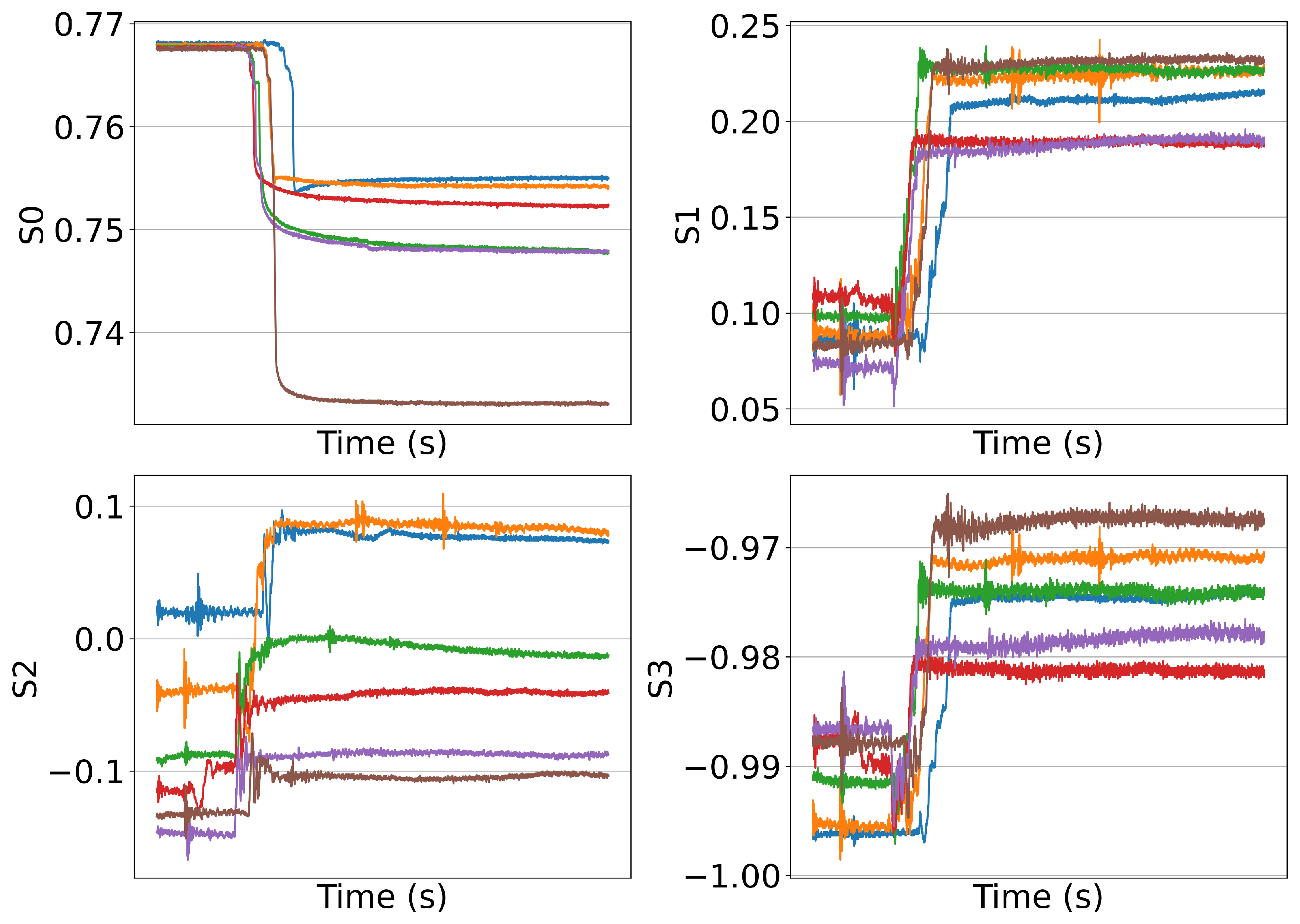
Figure 2.
Simultaneous occurrence of bending and tapping
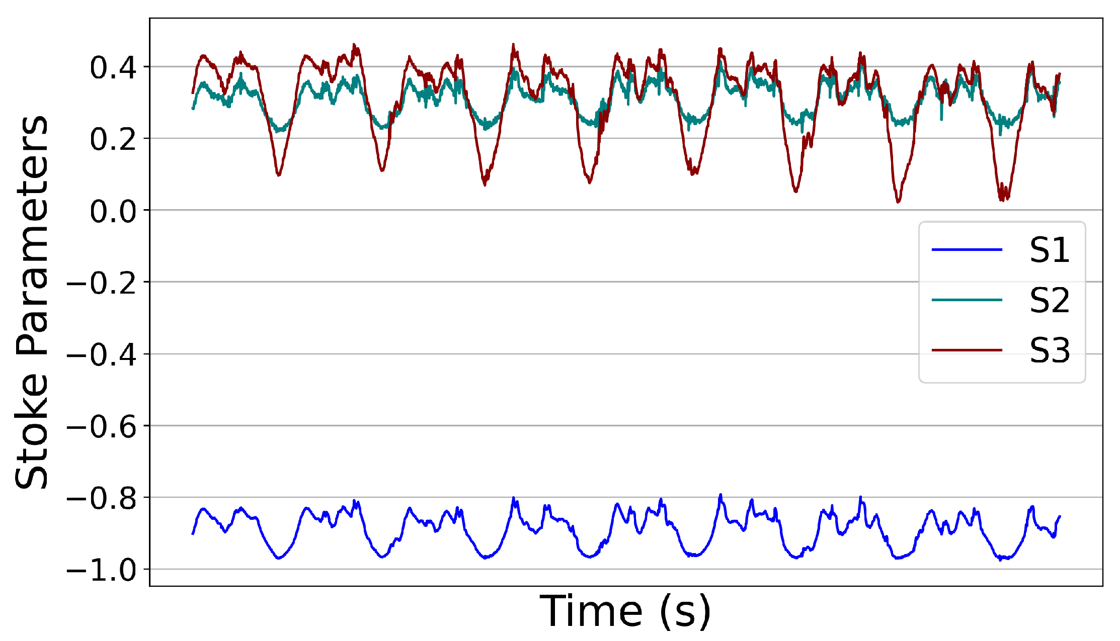
Figure 3.
stoke parameters plot for the clean dataset
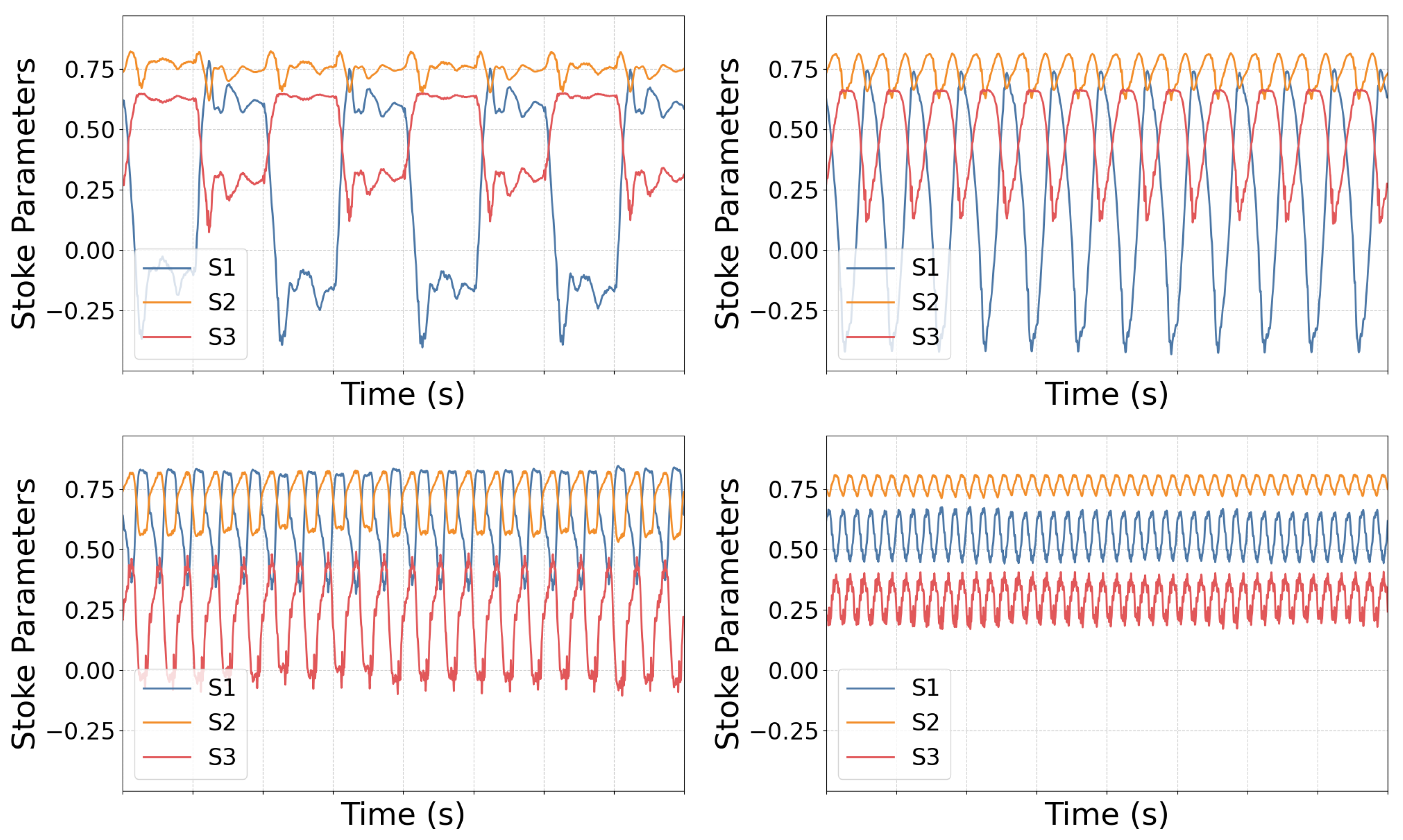
Figure 4.
Stokes Parameter Variations Under 3 Hz Noise Perturbation
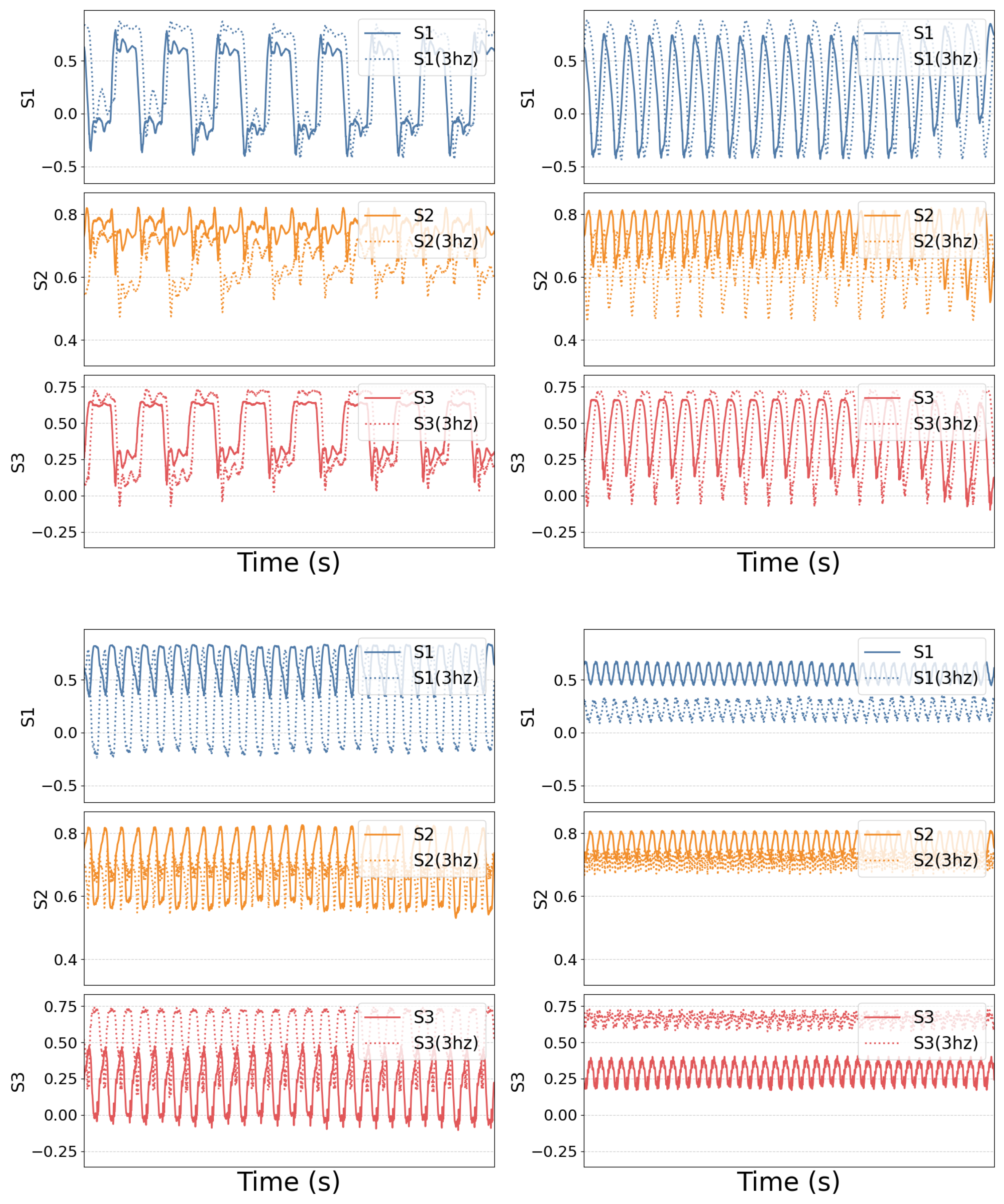
Figure 5.
Flowchart of the machine learning framework for predictive modeling.
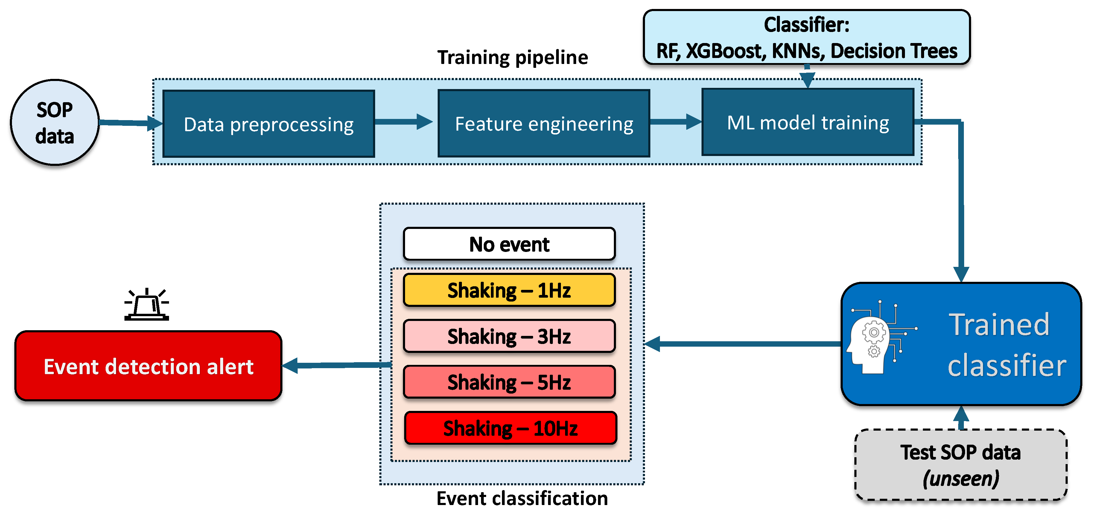
Figure 6.
Comparison of Metrics of the Models trained on the clean dataset.
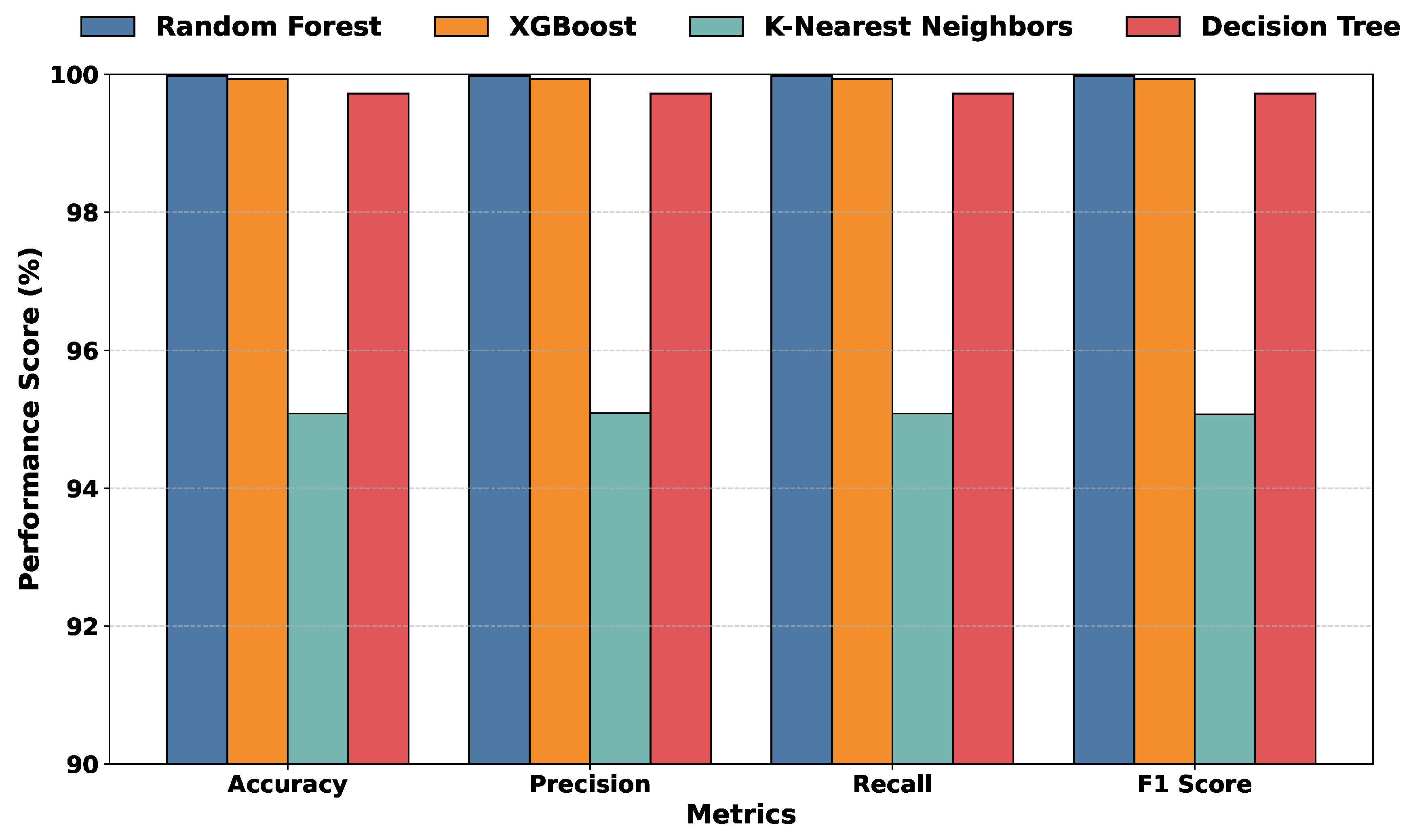
Figure 7.
Confusion metrics of all the models after testing on the clean data.
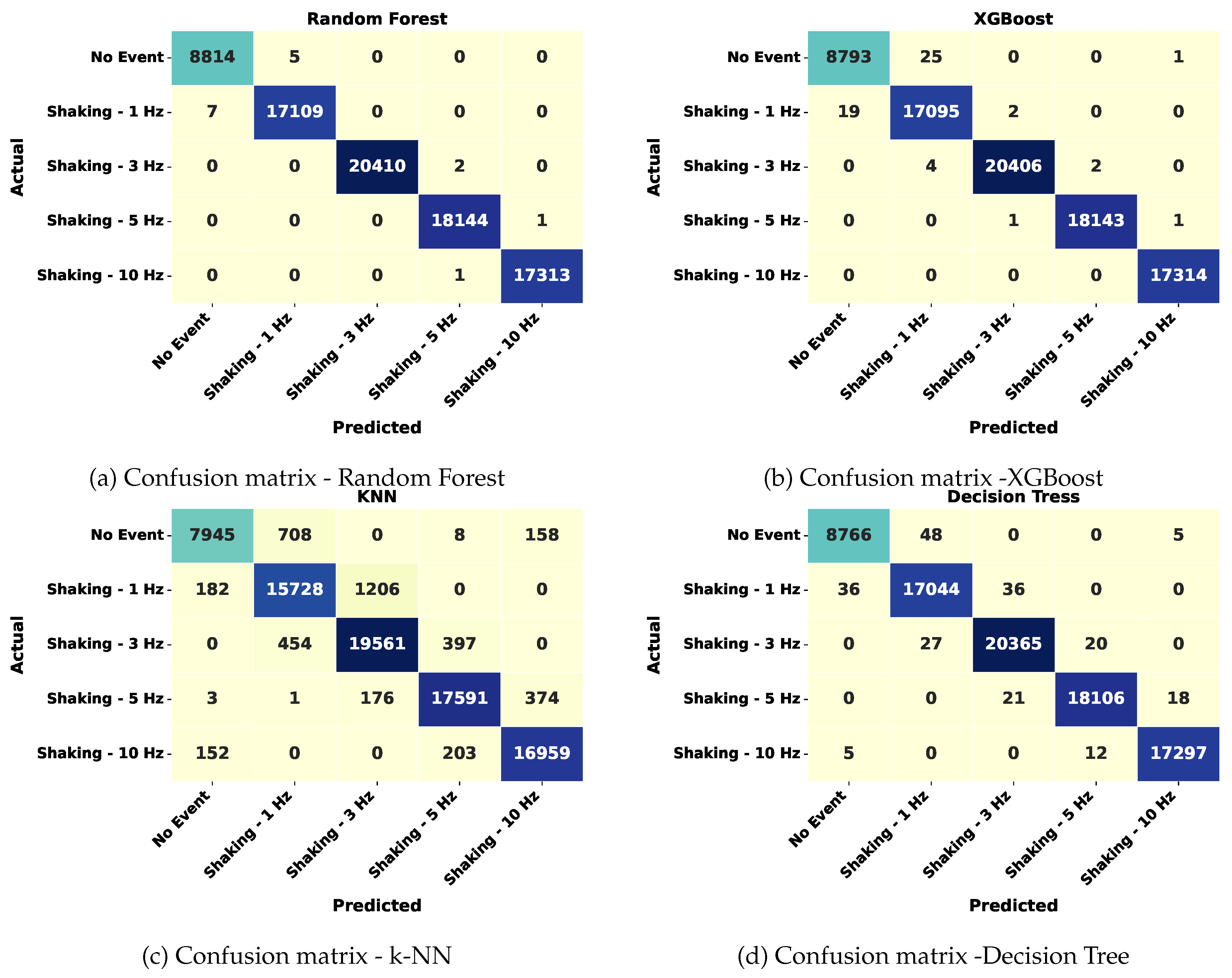
Figure 8.
Accuracy scores of the Random Forest model tested on the datasets with various noise levels.
Figure 8.
Accuracy scores of the Random Forest model tested on the datasets with various noise levels.
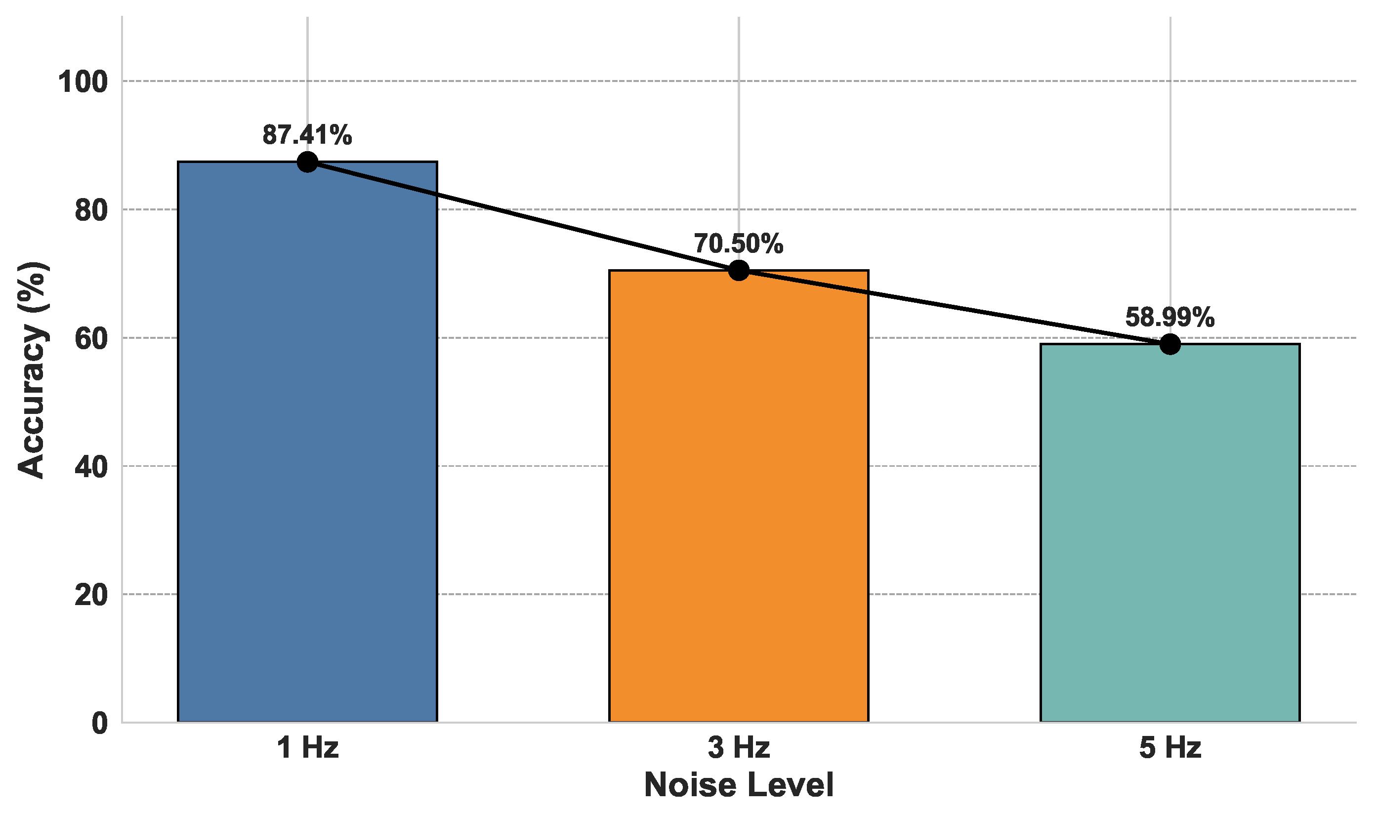
Figure 9.
Confusion matrix for testing on different noise levels
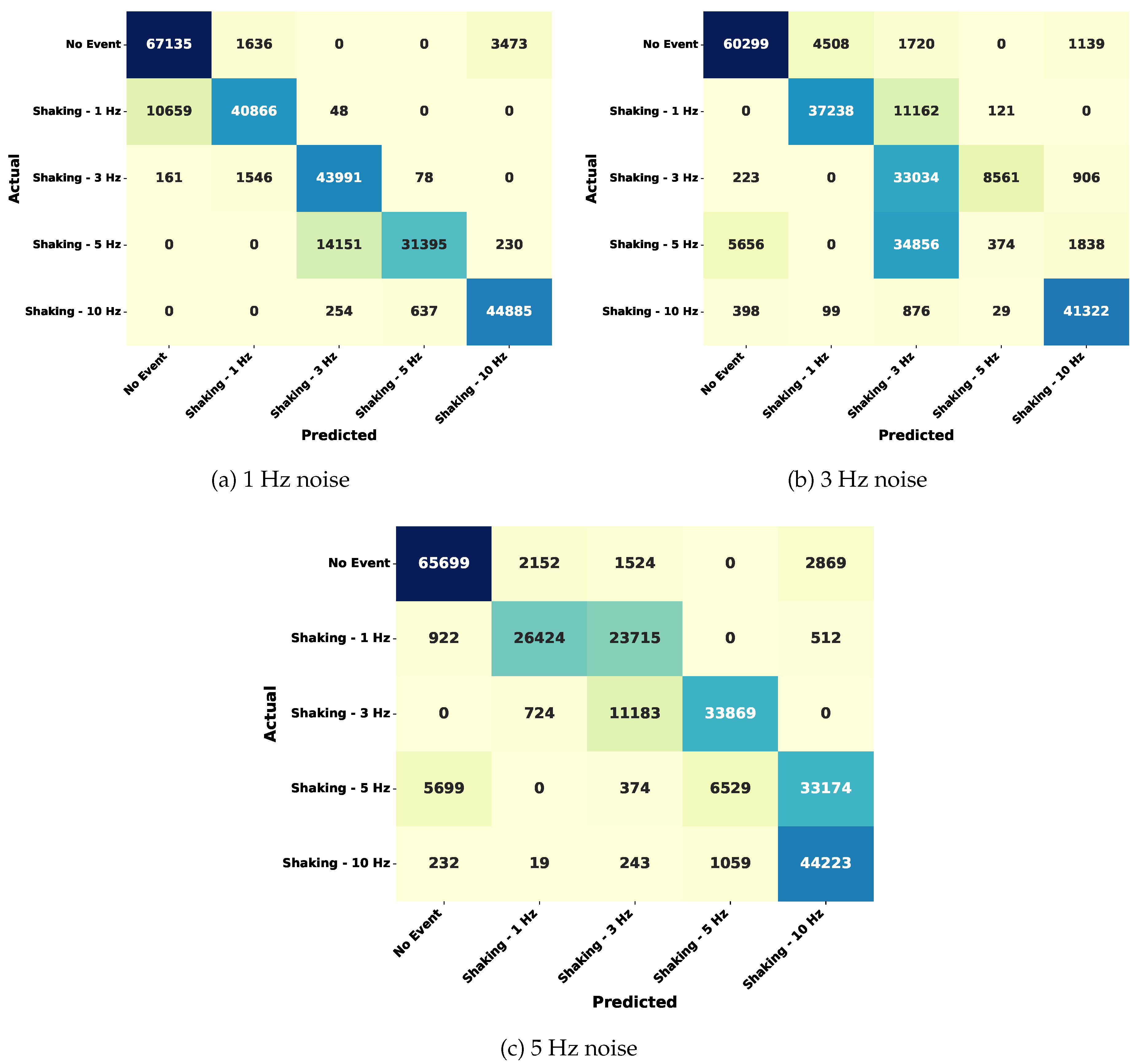
Figure 10.
Comparison of per event accuracy of clean data with different noise levels
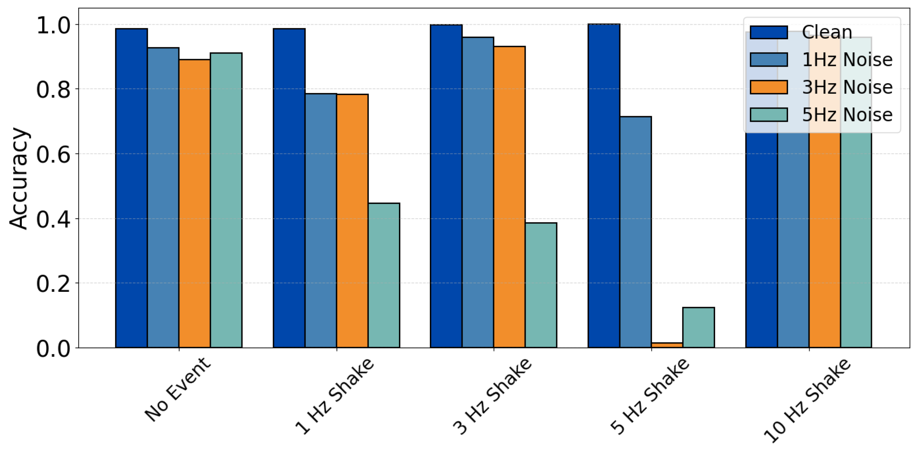
Figure 11.
Radar plot of WPM scores illustrating accuracy–efficiency trade-offs.
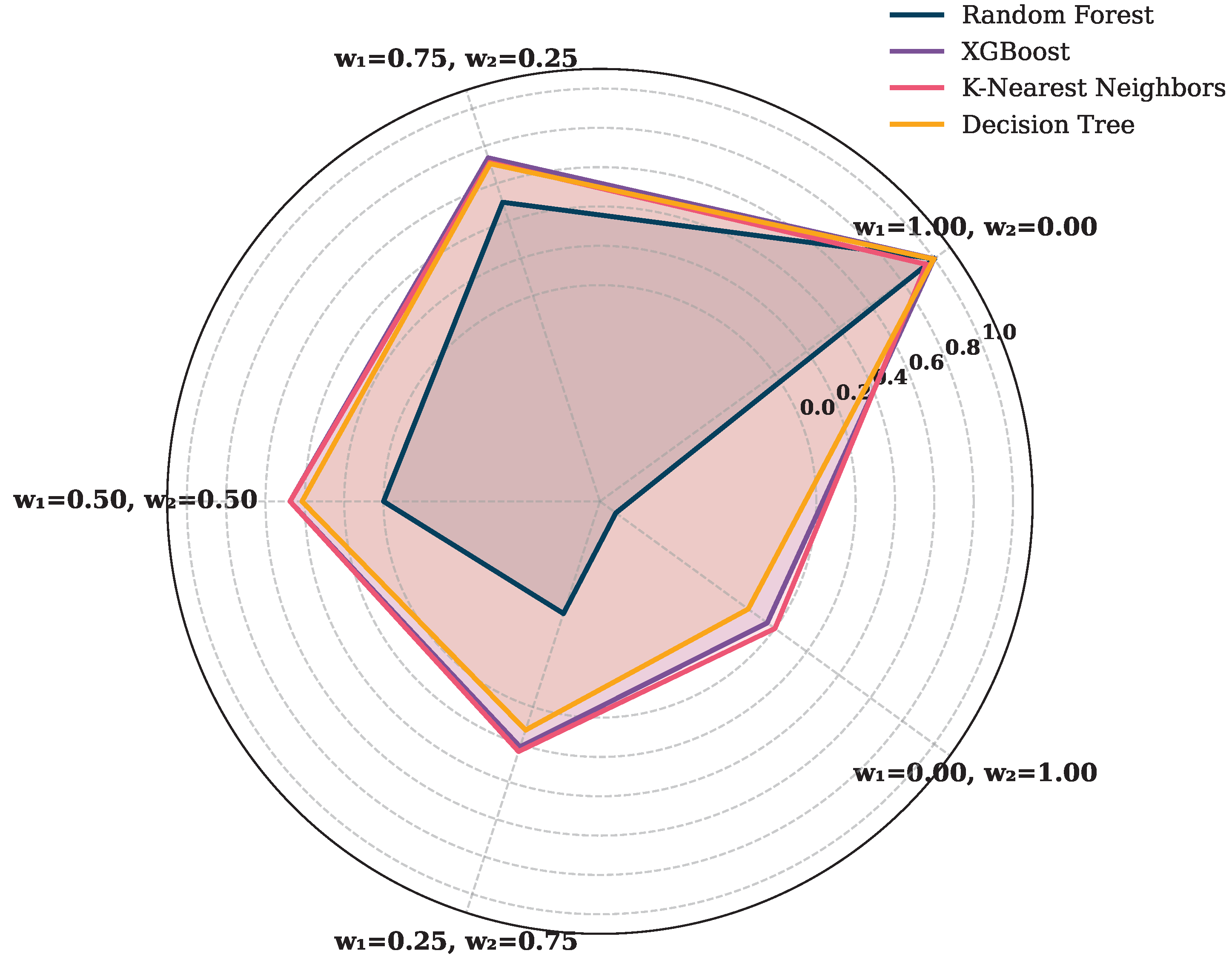

Table 1.
Categorization of Vibration Events
| Event Type | Severity Level | Description |
|---|---|---|
| No event | None | Normal operations with no impact on fiber integrity |
| Shaking (1Hz) | Low | Ambient noise due to environmental activities |
| Shaking (3Hz) | Moderate | Minor disturbances caused by nearby environment |
| Shaking (5Hz) | High | Sustained mechanical stress |
| Shaking (10Hz) | Critical | Critical intrusion |
Table 2.
Structure of Confusion Matrix
| Predicted Positive | Predicted Negative | |
|---|---|---|
| Actual Positive | TP | FN |
| Actual Negative | FP | TN |
Disclaimer/Publisher’s Note: The statements, opinions and data contained in all publications are solely those of the individual author(s) and contributor(s) and not of MDPI and/or the editor(s). MDPI and/or the editor(s) disclaim responsibility for any injury to people or property resulting from any ideas, methods, instructions or products referred to in the content. |
© 2025 by the authors. Licensee MDPI, Basel, Switzerland. This article is an open access article distributed under the terms and conditions of the Creative Commons Attribution (CC BY) license (http://creativecommons.org/licenses/by/4.0/).
Copyright: This open access article is published under a Creative Commons CC BY 4.0 license, which permit the free download, distribution, and reuse, provided that the author and preprint are cited in any reuse.


