
Submitted:
21 May 2025
Posted:
21 May 2025
You are already at the latest version
Abstract
Environmental monitoring systems often operate continuously, measuring various parameters, including carbon dioxide levels (CO2), relative humidity (RH), temperature (T), and other factors that affect environmental conditions. Such systems are often referred to as smart systems because they can autonomously monitor and respond to environmental conditions and can be integrated both indoors and outdoors to detect, for example, structural anomalies. However, these systems typically have high energy consumption, data overload, and large equipment sizes, which makes them difficult to install in constrained spaces. Therefore, three challenges remain unresolved: efficient energy use, accurate data measurement, and compact installation. In this study, we propose a 2-to-1 threshold sampling approach, where the CO2 measurement is activated when the specified T and RH change thresholds are exceeded. The proposed approach was implemented on a low-power, small-form and self-made multivariate sensor based on the PIC16LF19156 microcontroller. In contrast, a commercial monitoring system and sensor modules based on the Arduino Uno were used for comparison. As a result, by activating only key points in the T and RH signals, the number of CO2 measurements was significantly reduced without loss of essential signal characteristics. Signal reconstruction from the reduced points showed acceptable accuracy, as confirmed by the results of calculating Mean Absolute Error (MAE) and Root Mean Squared Error (RMSE).
Keywords:
structural health monitoring
; multivariate sensors
; event-driven activation
; data reduction
; energy efficiency
1. Introduction
There is a growing interest in the analysis of the environment and its impact on the condition of building structures. The interest is due to the fact that environmental factors have a direct impact on the condition of structures and the service life of materials. Parameters such as temperature (T), humidity (), and carbon dioxide () are recognized as key properties for assessing the impact on material degradation processes and the general condition of building structures [1,2]. Understanding the role of each of these parameters helps to assess their influence on structural behavior and interaction with the environment. T and indicate the thermodynamic characteristics of the environment, reflecting the distribution of heat and steam exchange, and is a key indicator of air quality or gas accumulation in buildings, since its constant concentration can affect the pattern of the so-called carbonation of concrete (in case the building is made of concrete structures) [3,4]. Therefore, all these parameters are considered together, since their behavior can be interrelated. For example, increased humidity can indicate increased dampness, insufficient ventilation, or a problem with thermal insulation leading to mold formation. An increase in can indicate occupancy or poor ventilation in the room, and a decrease in temperature can indicate a loss of structural integrity or a sign of poor heating system performance [5,6]. To collect and interpret such environmental indicators, appropriate sensor technologies are required. Sensor technologies are one of the key tools for implementing SHM, offering a variety of solutions for monitoring the condition of bridges, tunnels, and other critical infrastructure facilities [8,9]. A key element of these technologies is the continuous monitoring of environmental conditions such as deformation, temperature, vibration, and gas concentration, allowing for early analysis of potential signs of material degradation, indoor gas accumulation, or ventilation failure [10,11]. Sensor systems that measure these three parameters simultaneously typically require a continuous power source. In particular, measurements require longer measurement times, since accuracy depends on a short calibration period [7]. In contrast, temperature and humidity sensors typically offer faster response times and are often considered to be basic parameters in monitoring systems [13]. Therefore, stable and continuous measurement of all these parameters becomes particularly important in the context of structural health monitoring, where long-term environmental trends need to be accurately monitored to identify potential risks to structures [14]. Another important issue is the efficient processing of sensor data, beyond measurement accuracy. To ensure the reliability of such sensor systems, not only the detection mechanism but also data management is of critical importance. Evenly distributed use of memory for storing sensor data is critical, as memory overflow can lead to poor performance and, in some cases, hardware failure [15]. Additionally, the simultaneous processing of large amounts of data increases the computational load, resulting in higher power consumption, which is especially critical in low-power or embedded sensor systems [33]. Moreover, data reduction in real-time measurements is another crucial issue in sensors with limited hardware resources, since acquiring data, analyzing it quickly, and storing important points at the same time requires significant computational effort. In this regard, several studies have applied data compression techniques that involve data collection, filtering, signal sampling, and removal of unimportant signals [19]. All of these challenges are largely due to the inefficiency of traditional sensor systems. Traditional sensor systems operate on a fixed time base, where all parameters are measured at fixed intervals, regardless of whether a specific event has occurred in the environment or not. Although such a process ensures the integrity of the measured data, it results in unnecessary measurements, increased storage space, and depletion of the power supply (e.g., batteries). Many studies rely on cloud-based systems, where the hardware of the sensor system is processed and the data is stored in the cloud [17,18], but this is difficult to implement in the context of low-power sensors. To optimize data storage, a data reduction method has been proposed [20]. Machine Learning methods have also been proposed, but they require high computing power to train and execute on big data. In this context, recent studies have also shown the ability to reduce power consumption in sensor network systems by activating a master sensor, the so-called agent, which gives the activation command to other sensors [21]. However, even the passive state of sensors leads to constant energy consumption, especially if the sensor includes several parameters such as humidity, , gas, and temperature. To address this issue, we propose a method aimed at reducing unnecessary dimensions by implementing an adaptive sampling strategy. Specifically, we propose a method that uses temperature and humidity to selectively activate the parameter. The objective is to avoid constant response to the environment and trigger a measurement only when either parameter changes above a predefined threshold. First, this approach reduces the frequency of temperature and humidity measurements based on the threshold, resulting in energy savings. Second, it is particularly suitable for resource-constrained sensors. The method was implemented as an algorithm and integrated it into our custom multivariate sensor. Unlike many existing methods, this approach eliminates the need for machine learning, which is often impractical in conditions of limited hardware resources. The results show that a significant reduction in humidity measurements can be achieved without losing critical information. This contributes not only to data efficiency but also to extending the lifetime of battery-powered sensor devices. Three different sensor were used in this study, which are referred to below as follows: Sensor 1 – a commercial Loxone monitoring system; Sensor 2 – a custom-designed module based on a PIC16LF19156 microcontroller; Sensor 3 – an Arduino Uno-based platform with DHT22, DS18B20 and MQ-135 sensors.
2. Materials and Methods
This section describes the experimental materials, sensor types, the proposed approach, and the evaluation of the methods. First, existing data optimization methods are assessed. Then, the three sensor type (Sensor 1, Sensor 2, and Sensor 3) are described in detail, focusing on their configurations and data acquisition procedures. Then, the selected environmental conditions and sensor installation locations are described. Next, the logic of the proposed approach as an event based measurement method is presented, as well as the rationale for activating sampling based on humidity () and temperature (T) thresholds. Finally, the data processing and signal reconstruction evaluation strategy is explained, including the mean absolute error (MAE) metric.
2.1. Baseline Methods for Data Reduction
Before starting the experiments, existing time series simplification methods were reviewed and tested to create a performance baseline, which allowed us to subsequently evaluate what reduction could be achieved using our method. The performance of each method was assessed by comparing the reduced and original signals (R) using the mean absolute error (MAE) as a measure of reconstruction accuracy, with the results shown in Table 1. For example, when applying the Ramer–Douglas–Peucker (RDP) [32] algorithm to our collected data of approximately 3,000 data points, only 960 points were retained after simplification, resulting in a reduction of approximately 68%.
where is the total number of data points before reduction and is the number of data points after the reduction method. To assess the accuracy of the reconstruction, we interpolated the reduced signal back to the original time axis and calculated the mean absolute error (MAE) between the original and reconstructed signals.
where is the original value and is the reconstructed value at index i and n is the total number of observations. Using this metric, each method in the table was applied to the same set of sensor data. According to our observations, those with higher MAE and lower data reduction rates were not included in the table. As a result, this review allowed us to determine how each approach can recover from reduction or whether it is possible to use it as a hybrid with our approach, especially in the context of low-power sensors. For example, principal component analysis (PCA) can be used as a complement to reduce the dimensionality of data in memory, thereby increasing storage capacity [31]. In general, combining several methods with our proposed approach may be the next step in implementation, especially when developing on more powerful microcontrollers (for example PIC16LF19186 [30]).
2.2. Sensor Setup and Experimental Environment
The initial objective of this study was to find a suitable location to ensure proper analysis from different locations and to place sensors to collect environmental data. For this selection, three types of places were selected, those located away from the city (with minimal influence of urban factors such as road vibration and noise) (see Figure 1) and rooms within buildings located inside the city, where one room has a frequent presence of people, while the other is often empty (see Figure 2).
These conditions allowed us to compare different climate parameters under varying levels of external influence. All measurements were carried out over a period of one month, with sensors placed between two structural elements in the house and others in the corner of a wall inside the building. This arrangement allowed us to record changes in T, H, and , including increases, decreases, and sharp fluctuations. As part of the monitoring setup, we used the commercial smart system Loxone, which was configured to measure three parameters simultaneously: temperature, humidity, and concentration.
The next sensor, designed specifically for integration in hard-to-reach places, also measures three parameters simultaneously (see Figure 3). This sensor is based on the PIC16LF19156, has built-in flash memory for local data logging, and has an optional connectivity module. The connectivity components include a digital temperature and humidity sensor and a non-dispersive infrared sensor. The sensor was originally designed for use in industrial environments where energy-efficient operation and modular integration are important. And the third measuring device was a simple one based on Arduino Uno, where separate , T and modules were connected. All modules were connected to a breadboard, where the code was subsequently written to measure the environment and the data was stored in a built-in flash card module.
Each sensor consists of several key components, each of which has specific parameters for measuring the environment. The advantage of the PIC16LF19156 microcontroller is its low power consumption, compact size and the presence of necessary peripheral modules, such as ADC, UART and built-in EEPROM. A component based on the HS4111 was used to measure T and H, which operates in the range of to with an approximate accuracy of for T, and from to with an accuracy of . To obtain a low-noise signal, a 12-bit ADC converter was used, buffered by a 10MHz analog front end. levels were measured using an STC-C4 sensor, which has a detection range of 400 to 5000ppm and an accuracy of ppm. The module, which stores three parameters, is equipped with a UART communication interface and is integrated via a serial connection with a PIC16LF19156 microcontroller. A real-time clock (RTC) was included for reliable readings. Among other parameters, the sensor included a 3-axis accelerometer (ADXL325) with a measurement range of to detect events based on motion or vibration (this was prepared for real integration in confined spaces or embedded equipment). The sensor also includes a light component (SFH5711 photodiode) for day-night transition conditions. The sensor architecture is modular, supports both analog and digital interfaces, and is equipped with a 6-channel analog interface and I2C communication for sensor expansion. An Arduino-based data acquisition system was developed using several modules: DHT11 for humidity and moisture, DS18B20 for temperature measurement, and MQ-135 as a gas sensor capable of detecting . As for the Arduino Uno platform, three sensor modules were used: a DHT22-based humidity sensor, a 4-digit temperature sensor, and an MQ-135 gas sensor for . The humidity sensor operates in the range of 20–60%RH with an approximate accuracy of 5% and a response time of 5–10 seconds under stable airflow conditions. The DS18B20 is a 1-Wire digital temperature sensor that operates from to with a typical accuracy of over the range of to . The MQ-135 sensor was used to monitor indirectly through its chemical sensitivity to several gases (e.g. , alcohol and ). All modules were connected via a breadboard to an Arduino Uno, and data were collected via a serial line monitoring in real time. And for Loxone, the sensor operates in the temperature range from –20 °C to +55 °C and can resist relative humidity up to 95%. The connection is established via the Loxone Tree interface, which allows for direct integration with the Loxone Miniserver or Tree Extension module. The sensor is also capable of detecting temperatures in the range from –40 °C to +120 °C with an accuracy of ±0.5 °C, and relative humidity from 0% to 100% r.H. with an accuracy of ±2% (without condensation). For CO2 monitoring, the sensor operates in the range with a detection range of 400–10,000 ppm and an accuracy of ±(30 ppm + 3%).
2.3. Data Acquisition
In the data acquisition stage, data collection was performed in parallel using three sensors, each programmed to measure all three parameters — temperature, humidity, and at intervals ranging from 1 to 15 minutes. The observation period lasted for one month (Sensor 1 and Sensor 3: March; Sensor 2: April), enabling the recording of a complete time profile of environmental parameter changes. For example, in Sensor 3, data were saved to memory (SD card), while in Sensor 2, data were transmitted directly via USB. In Sensor 1, data were written to the internal memory of the controller. All collected values were subsequently visualized, allowing for an analysis of the relationships between the parameters. To provide a clearer understanding of how the measurements were obtained and structured, the data collection process is described in more detail below. As for Sensor 1, the data were automatically exported in CSV format, and owing to its accuracy and stability, Sensor 1’s data did not require additional pre-processing before time-series analysis (see Figure 4).
As for the Sensor 3, the data collection program was written using the Arduino IDE with libraries such as DHT.h, OneWire.h, and MQ135.h to communicate with the sensors. Data readings were collected every 15 minutes, and saved to the SD card, where it was later stored in CSV format. It is worth noting here that the data was also slightly processed using Python, which included libraries such as pandas, numpy, and matplotlib for pre-processing and visualization (see Figure 5).
Simultaneously, data were collected using a custom-designed sensor based on a PIC16LF19156 microcontroller and a program written in MPLAB X IDE using the Microchip Code Configurator (MCC), with a particular focus on three types of sensors: a humidity sensor, a digital temperature sensor (e.g., DS18B20), and a STCC4-based sensor. The resulting data were time-stamped and missing values were handled using direct interpolation. Matplotlib, seaborn and scipy were used for data analysis (see Figure 6).
2.4. Correlation
A critical component of the methodology involves analyzing of the relationships between the environmental parameters. The goal is to determine whether T and contain enough information about the behavior of to act as triggers, or whether T and have a better relationship to be used as triggers for one parameter. For this purpose, a correlation analysis was applied to the parameters using the data collected from three sensors. It is necessary to determine how consistently changes in temperature and humidity are associated with fluctuations in the concentration of , and how reliable these two parameters can be without regularly measuring . If a pronounced correlation is detected, then the two parameters can serve as a reliable basis for predicting the behavior of the third parameter.
Based on the correlation matrix (see Figure 7), the data obtained from Sensor 2 demonstrate a weak positive correlation between T and (), and between and (). According to the data from Sensor 3, there is a strong correlation between T and (), while the correlation between and is also positive but weaker (). However, T and are practically unrelated to each other (). The dataset from Sensor 1, however, represents a positive correlation between T and (), but is practically independent of both parameters ( with T and with ). As a result, two of the sensors revealed a positive correlation between temperature, humidity, and concentration. This allows these parameters to be used as a basis for developing trigger logic for activating the measurements.
For further confirmation of the correlation analysis, a combined pairplot was constructed (see Figure 8), illustrating the distribution and interrelation of the parameters from each sensor’s dataset. This is particularly important when constructing the trigger activation logic. The pairplot shows that temperature and humidity in the Sensor 1 and Sensor 2 data are concentrated within a narrow range, while Sensor 3 demonstrates a more uniform distribution. in all three cases exhibits a pronounced right-hand shift, indicating the passive presence of people in the premises. The data from the Sensor 2 and sensor 3 show a positive trend between temperature and , which is consistent with the previously obtained correlation matrix. The data from Sensor 1, however, show less pronounced relationships between temperature and , with a chaotic scattering of points, confirming a weak correlation.
2.5. Trigger Justification
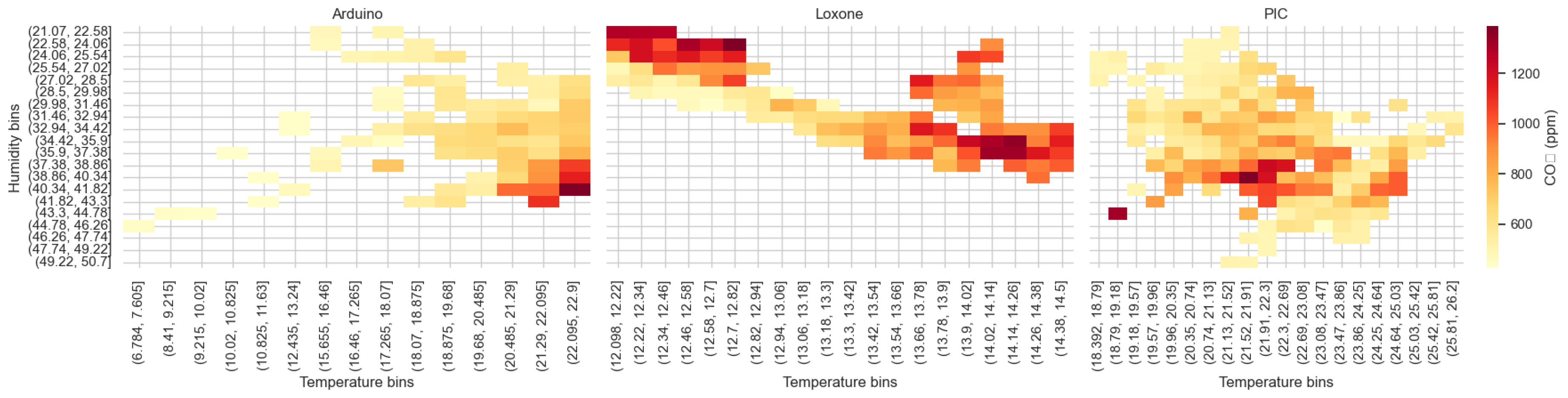
As a further step in the analysis of the influence of temperature and humidity on the levels, a two-dimensional heat map was constructed based on the partitioning of the two parameters into discrete intervals. The horizontal axis represents the temperature intervals, and the vertical axis the humidity intervals. The color of each cell shows the average value of concentration for a combination of temperature and humidity values. According to the data from Sensor 3, exceeds 1000 ppm in the region corresponding to temperatures of 21–22.5°C and humidity levels of 37–41%. This indicates that increasing temperature and humidity are suitable triggers for measurement. Similarly, the data from Sensor 2 a stable trend of increasing with increasing temperature (>21°C) and humidity. In contrast, the data from Sensor 1 show a very weak correlation, though temperature and humidity may still be used as a combined trigger for sampling.
Figure 9.
Heat map of average concentration across temperature and humidity intervals.
Building on this observation, the main proposed approach, which is based on "two to one" - involves activating one parameter (in this case ) based on the behavior of the other two (T, ). Within this pattern, two parameters are monitored simultaneously and if the change in each of them exceeds a set threshold or a checkpoint in time is reached, then the third parameter is measured. To formalize this concept, let define three parameters as : T at time t, : at time t and : . , be the threshold values for and . represent the absolute change in parameter at time t. be a fixed control interval (e.g., every 20 time steps). The conditional activation rule for measuring y is defined as:
where means that at time step t, a new measurement of is executed.
2.6. Threshold Selection
After two parameters have been approved as trigger parameters for the activation of the third parameter measurements, the next process is to determine the threshold values. A grid search was used to select the thresholds, and the Precision, Recall, and the F1 Score quality metrics were computed for each combination. Precision measures how many of the triggered events were true for CO2 peaks, recall measures how many actual CO2 peaks were correctly detected, and the F1 score is the harmonic mean of precision and recall, used to balance of both metrics:
Based on the grid search described above, we systematically evaluated all relevant combinations of temperature and humidity thresholds. The combination that achieved the highest F1 Score was selected as the optimal trigger condition, and the following thresholds were determined: the temperature threshold is C, and the humidity threshold is . This threshold pair yielded the best trade-off between precision and recall, achieving an F1 Score of 0.473, with a trigger rate of 95.4%. This means that most high events were successfully detected, although with a relatively frequent activation rate. The selected thresholds were used throughout the trigger behavior simulation and system implementation on the PIC-based sensor platform. The top five threshold combinations including precision, recall, F1 score, and triggering rates are presented in Table 2. As shown, several threshold pairs resulted in nearly identical F1 scores.
To better visualize the overall performance, Figure 10 presents the heatmap of the F1 Score, which clearly highlight areas with the best activation accuracy.
3. Results
As shown in the Figure 11, the upper part displays a sharp increase in . The middle and lower panels display the temperature and humidity signals. The dashed lines indicate the activation thresholds (20.5°C and 31%). The black markers indicate the moments when both thresholds are exceeded simultaneously, thereby activating the measurement. In the next graph, a more visual representation of the reconstructed signal from the reduced data is presented.
After triggering the measurements based on certain thresholds, the reduced data were used to reconstruct all parameters. The resulting reconstruction is visualized in the Figure 12, demonstrating that the main signal characteristics were preserved despite the lower sampling rate.
Returning to our original question of how much our measurement was reduced, the results in the accompanying Table 3 show the percentage of data points retained, as well as the corresponding reconstruction error measured in terms of MAE and RMSE.
4. Discussion
In this study, a threshold-based activation method for reducing measurements by 2-to-1 was proposed. The main goal of the proposed 2-to-1 method is to trigger the measurement of one parameter only when the thresholds of two other parameters are exceeded simultaneously. It is important to note that the trigger pair is not necessarily temperature and humidity, but can be combined depending on environmental events. In this experiment, temperature and humidity are the trigger parameters for . To evaluate the method, three different sensors were used that measured over a two-month period (March and April). The results showed the ability to reduce the data, but have several limitations. First, the analysis was conducted over a two-month period, which is a very short time to fully prove the choice of T and . For this, it is necessary to measure over the entire year in order to take into account all seasonal weather conditions, as well as changes in ventilation, the absence of people in the premises, weather variability, etc. Secondly, the use of static thresholds is limiting in the context of adaptive activations; the optimal solution would be to use a dynamic threshold mechanism that could adapt to all seasonal and temporal environmental events. Thirdly, it is important to note that readings may be more effective in the summer months. Finally, setting a smaller interval (every second) can improve the accuracy of detecting significant changes and improve the trigger response.
Author Contributions
Conceptualization, C.E. and N.D.; methodology, S.H., C.E. and N.D; software, N.D.; validation, S.H., C.E. and N.D.; formal analysis, N.D.; investigation, C.E. and N.D; resources, C.E.; data curation, N.D.; writing—original draft preparation, N.D.; writing—review and editing, N.D.; visualization, N.D.; supervision, S.H.; project administration, C.E. and N.D.; funding acquisition, S.H. All authors have read and agreed to the published version of the manuscript.
Institutional Review Board Statement
Not applicable.
Data Availability Statement
Data used in this study are not publicly available but can be obtained from the authors upon request.
Conflicts of Interest
The authors declare no conflict of interest.
References
- Liu, P.; Chen, Y.; Yu, Z. Effects of temperature, relative humidity and carbon dioxide concentration on concrete carbonation. Mag. Concr. Res. 2019, 72, 936–947. [Google Scholar] [CrossRef]
- AL-Ameeri, A.S.; Rafiq, M.I.; Tsioulou, O.; Rybdylova, O. Impact of climate change on the carbonation in concrete due to carbon dioxide ingress: Experimental investigation and modelling. J. Build. Eng. 2021, 44, 102594. [Google Scholar] [CrossRef]
- Leemann, A.; Moro, F. Carbonation of concrete: The role of CO2 concentration, relative humidity and CO2 buffer capacity. Mater. Struct. 2016, 50, 30. [Google Scholar] [CrossRef]
- Chen, Y.; Liu, P.; Yu, Z. Effects of environmental factors on concrete carbonation depth and compressive strength. Materials 2018, 11. [Google Scholar] [CrossRef]
- Asif, A.; Zeeshan, M. Indoor temperature, relative humidity and CO2 monitoring and air exchange rates simulation utilizing system dynamics tools for naturally ventilated classrooms. Build. Environ. 2020, 180, 106980. [Google Scholar] [CrossRef]
- Sedoni, R.; Romani, M.; Santangelo, P.E. A hybrid model for the assessment of indoor environmental quality in buildings: An insight into mold growth. Energy Rep. 2025, 13, 4114–4125. [Google Scholar] [CrossRef]
- Zheng, Y.; Cao, L.-X.; Lv, J.-R.; Wen, H.-Y.; Mao, L.-X.; Wang, X.-Q.; He, Z.-Z. Self-powered flexible sensor network for continuous monitoring of crop micro-environment and growth states. Measurement 2025, 242, 116002. [Google Scholar] [CrossRef]
- Sofi, A.; Regita, J.J.; Rane, B.; Lau, H.H. Structural health monitoring using wireless smart sensor network – An overview. Mech. Syst. Signal Process. 2022, 163, 108113. [Google Scholar] [CrossRef]
- de Oliveira, V.P.; Reis, A.; Alves Salvador Filho, J.A. Assessing the evolution of structural health monitoring through smart sensor integration. Procedia Struct. Integr. 2024, 64, 653–660. [Google Scholar] [CrossRef]
- Solórzano, A.; Eichmann, J.; Fernández, L.; Ziems, B.; Jiménez-Soto, J.M.; Marco, S.; Fonollosa, J. Early fire detection based on gas sensor arrays: Multivariate calibration and validation. Sens. Actuators B Chem. 2022, 352, 130961. [Google Scholar] [CrossRef]
- Keshmiry, A.; Hassani, S.; Mousavi, M.; Dackermann, U. Effects of environmental and operational conditions on structural health monitoring and non-destructive testing: A systematic review. Buildings 2023, 13(4), 918, https://www.mdpi.com/2075-5309/13/4/918. [Google Scholar] [CrossRef]
- Zhang, T.; Wang, Z.; Wang, P. A method for compressing AIS trajectory based on the adaptive core threshold difference Douglas–Peucker algorithm. Sci. Rep. 2024, 14, 21408. [Google Scholar] [CrossRef]
- Abu Seman, M.T.; Abdullah, M.N.; Ishak, M.K. Monitoring temperature, humidity and controlling system in industrial fixed room storage based on IoT. J. Eng. Sci. Technol. 2020, 15, 3588–3600. [Google Scholar]
- Entezami, A.; Sarmadi, H.; Behkamal, B. Long-term health monitoring of concrete and steel bridges under large and missing data by unsupervised meta learning. Eng. Struct. 2023, 279, 115616. [Google Scholar] [CrossRef]
- Plageras, A.P.; Psannis, K.E.; Stergiou, C.; Wang, H.; Gupta, B.B. Efficient IoT-based sensor BIG Data collection–processing and analysis in smart buildings. Future Gener. Comput. Syst. 2018, 82, 349–357. [Google Scholar] [CrossRef]
- Sofianidis, I.; Konstantakos, V.; Nikolaidis, S. Reducing Energy Consumption in Embedded Systems Applications. Technologies 2025, 13, 82. [Google Scholar] [CrossRef]
- Shukla, A.; Somagattu, P.; Singh, V.; Kalra, M. IoT-Based Data Storage for Cloud Computing Applications. In Advances in Artificial Intelligence and Data Engineering; Chiplunkar, N.N., Fukao, T., Eds.; Advances in Intelligent Systems and Computing; Springer: Singapore, 2021; Volume 1133, pp. 1455–1464. [Google Scholar] [CrossRef]
- Leal Sobral, V.A.; Nelson, J.; Asmare, L.; Mahmood, A.; Mitchell, G.; Tenkorang, K.; Todd, C.; Campbell, B.; Goodall, J.L. A Cloud-Based Data Storage and Visualization Tool for Smart City IoT: Flood Warning as an Example Application. Smart Cities 2023, 6, 1416–1434. [Google Scholar] [CrossRef]
- Zhang, H.; Na, J.; Zhang, B. Autonomous Internet of Things (IoT) Data Reduction Based on Adaptive Threshold. Sensors 2023, 23, 9427. [Google Scholar] [CrossRef]
- Hwang, S.-H.; Kim, K.-M.; Kim, S.; Kwak, J.W. Lossless Data Compression for Time-Series Sensor Data Based on Dynamic Bit Packing. Sensors 2023, 23, 8575. [Google Scholar] [CrossRef]
- Abu Alsheikh, M.; Lin, S.; Niyato, D.; Tan, H.P. Machine Learning in Wireless Sensor Networks: Algorithms, Strategies, and Applications. IEEE Communications Surveys & Tutorials 2014, 16, 1996–2018. [Google Scholar] [CrossRef]
- Guo, C.; Li, H.; Pan, D. An Improved Piecewise Aggregate Approximation Based on Statistical Features for Time Series Mining. Adv. Data Min. Appl. 2010, 6440, 234–244. [Google Scholar] [CrossRef]
- Yang, D.-H.; Kang, Y.-S. Distance- and Momentum-Based Symbolic Aggregate Approximation for Highly Imbalanced Classification. Sensors 2022, 22, 5095. [Google Scholar] [CrossRef]
- Hu, T.; Huang, Z.; Ge, P.; Gao, F.; Gao, F. Adaptive De-noising of Photoacoustic Signal and Image Based on Modified Kalman Filter. arXiv 2022, arXiv:2211.10262. [Google Scholar] [CrossRef]
- Dai, B.; Frusque, G.; Li, Q.; Fink, O. Acceleration-Guided Acoustic Signal Denoising Framework Based on Learnable Wavelet Transform Applied to Slab Track Condition Monitoring. arXiv 2022, arXiv:2205.05365. [Google Scholar] [CrossRef]
- Bailey, J.; Smith, L.; Thompson, R. R Field Phase Shift Defect Signal Peak-to-Peak vs. Excitation Frequency. NDT E Int. 2022, 130, 102599. [Google Scholar] [CrossRef]
- Schweinzer, P. Variance Compression Leads to Participation Under Sufficient Variance Aversion. Eur. J. Oper. Res. 2021, 291, 1–10. [Google Scholar] [CrossRef]
- Upadhyaya, V.; Salim, M. Compressive Sensing: Methods, Techniques, and Applications. IOP Conf. Ser. Mater. Sci. Eng. 2021, 1099, 012012. [Google Scholar] [CrossRef]
- Jeon, G.; Chehri, A. Entropy-Based Algorithms for Signal Processing. Entropy 2020, 22, 621. [Google Scholar] [CrossRef]
- Microchip Technology. PIC16(L)F19155/56/75/76/85/86 Data Sheet; Microchip Technology Inc.: Chandler, AZ, USA, 2017; Available online: https://ww1.microchip.com/downloads/en/DeviceDoc/PIC16LF19155-56-75-76-85-86-Data-Sheet-40001923B.pdf. [Google Scholar]
- Gao, J.; Hu, W.; Chen, Y. Revisiting PCA for Time Series Reduction in Temporal Dimension. arXiv 2024, arXiv:2412.19423. [Google Scholar] [CrossRef]
- Sim, M.-S.; Kwak, J.-H.; Lee, C.-H. Fast Shape Matching Algorithm Based on the Improved Douglas–Peucker Algorithm. KIPS Trans. Softw. Data Eng. 2016, 5, 497–502. [Google Scholar] [CrossRef]
- Sofianidis, I.; Konstantakos, V.; Nikolaidis, S. Reducing Energy Consumption in Embedded Systems Applications. Technologies 2025, 13, 82. [Google Scholar] [CrossRef]
Figure 1.
Positioning of sensors in room corners in a historic manor house from the Wilhelminian period, adapted from Finn E. Schmid-Bonde, Fachhochschule Potsdam.
Figure 1.
Positioning of sensors in room corners in a historic manor house from the Wilhelminian period, adapted from Finn E. Schmid-Bonde, Fachhochschule Potsdam.
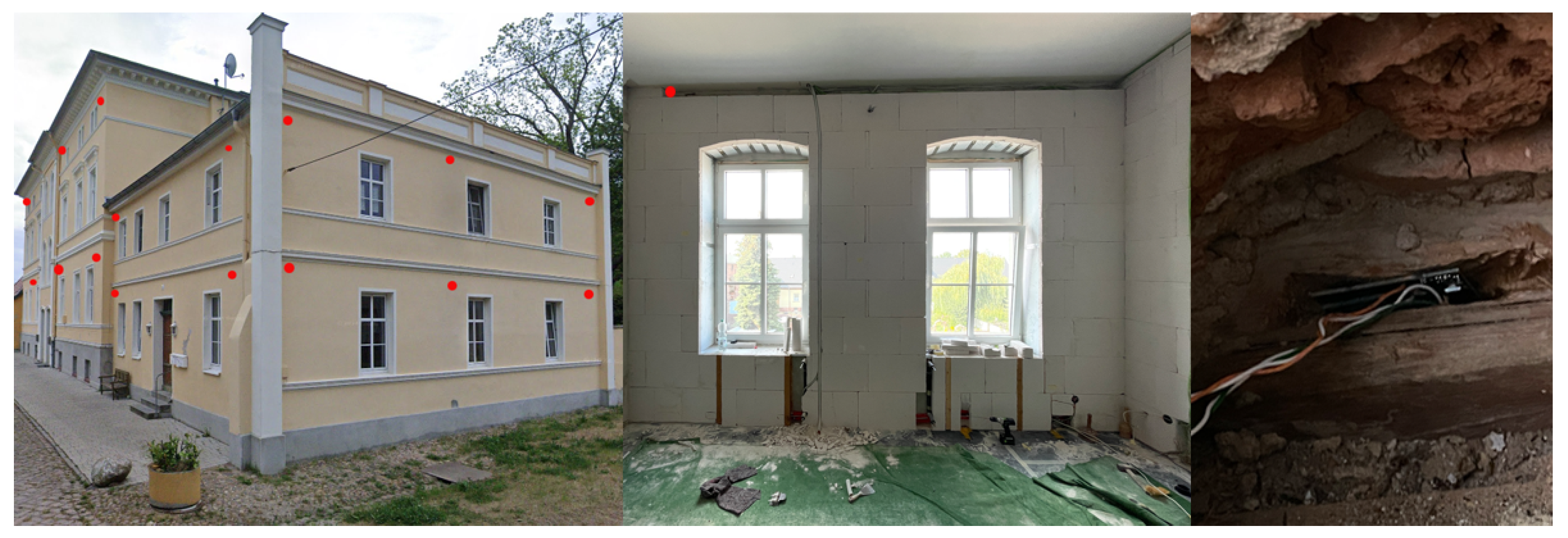
Figure 2.
Placement of sensors in two rooms within the same building: from left to right, the image shows the positions of the two monitored rooms.
Figure 2.
Placement of sensors in two rooms within the same building: from left to right, the image shows the positions of the two monitored rooms.
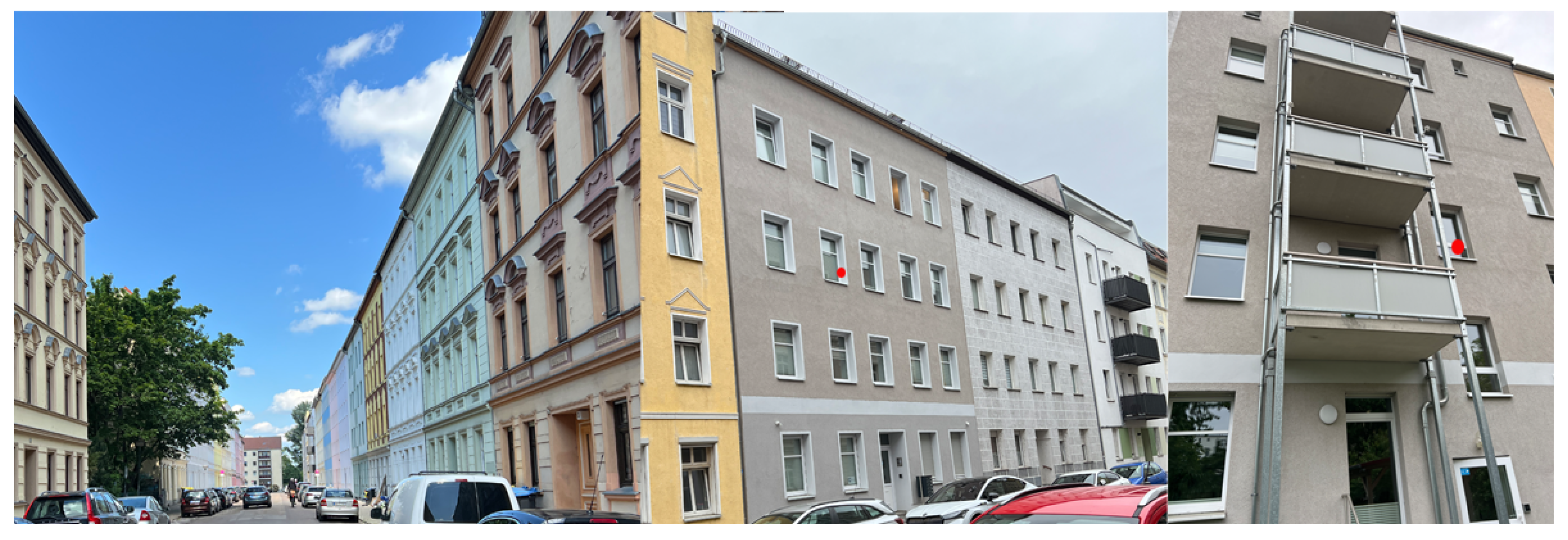
Figure 3.
From left to right: a custom PIC16LF19156-microcontroller-based (Sensor 1), Arduino based platform (Sensor 2) and Loxone smart system (Sensor 3).
Figure 3.
From left to right: a custom PIC16LF19156-microcontroller-based (Sensor 1), Arduino based platform (Sensor 2) and Loxone smart system (Sensor 3).
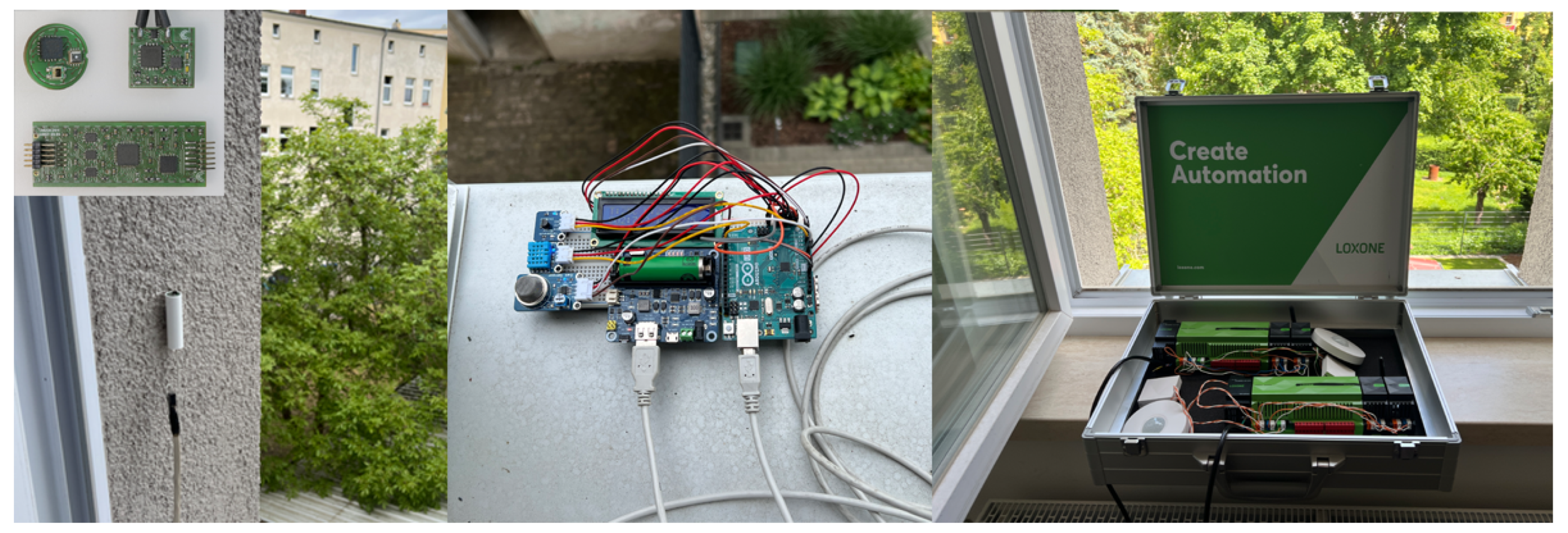
Figure 4.
Environmental data recorded by Sensor 1 during March.
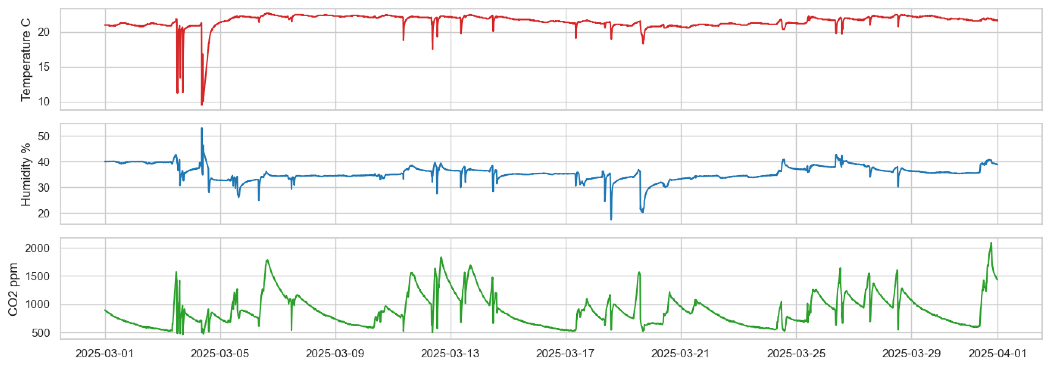
Figure 5.
Environmental data recorded by Sensor 3 during April.
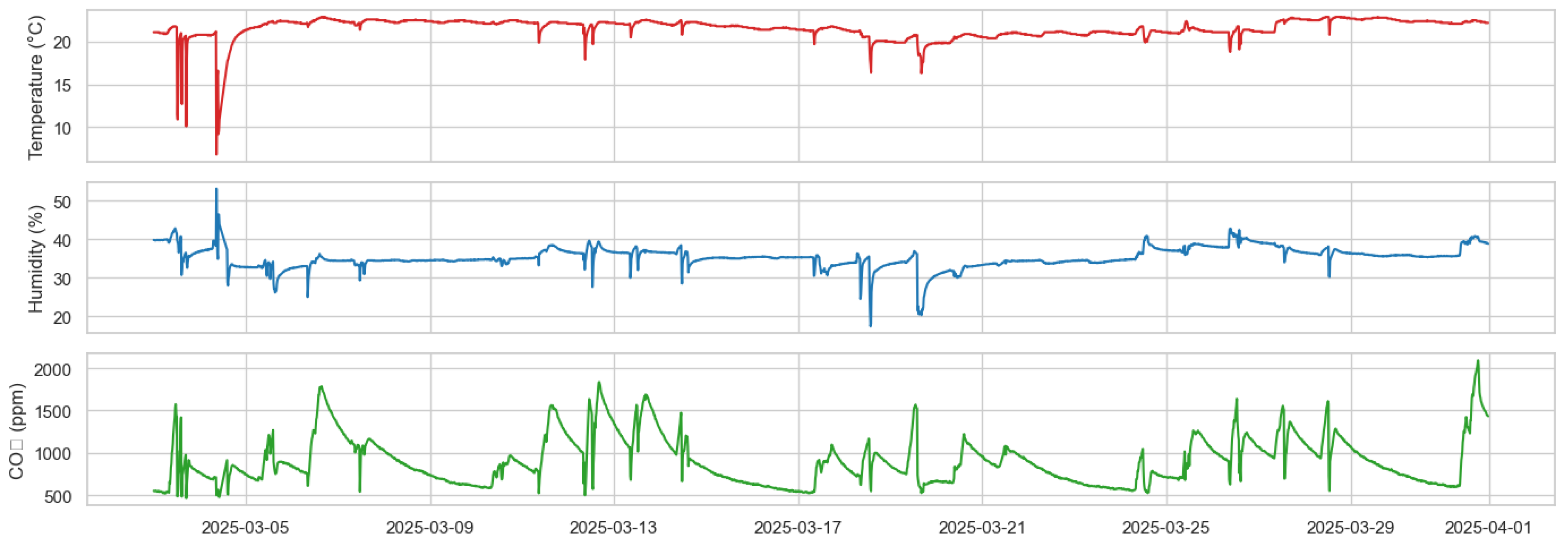
Figure 6.
Environmental data recorded by Sensor 2 during March.
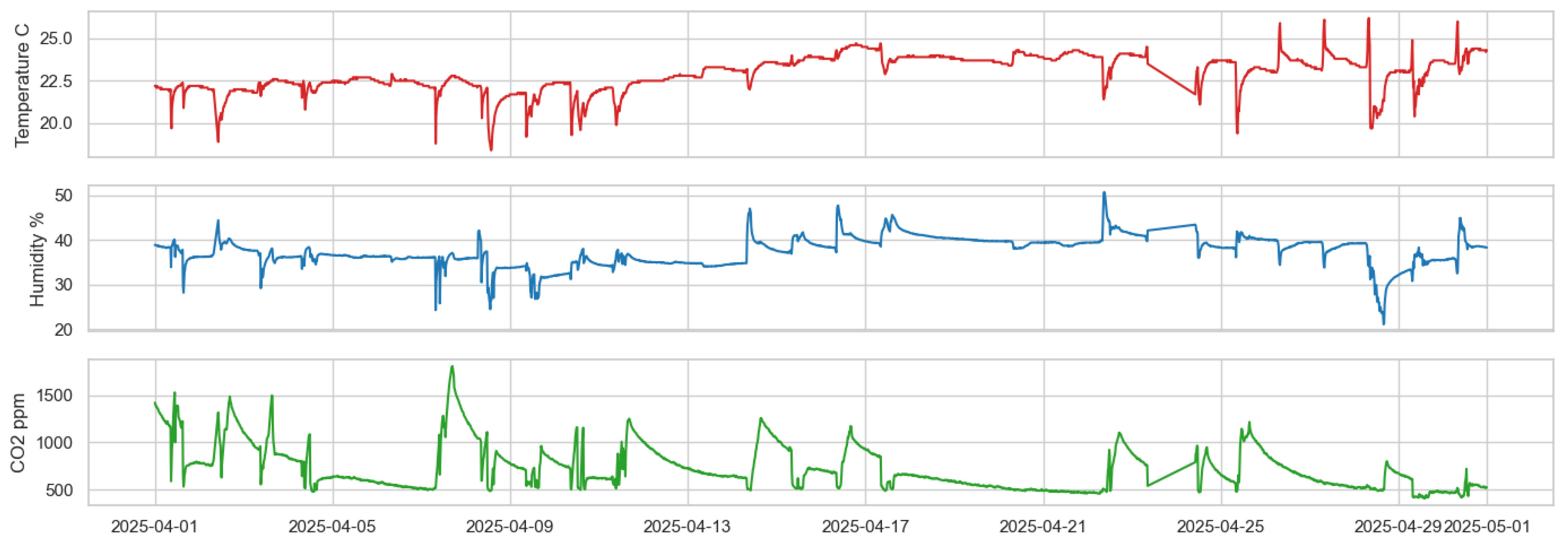
Figure 7.
Correlation matrix of environmental parameters (T, , ) for all three sensors
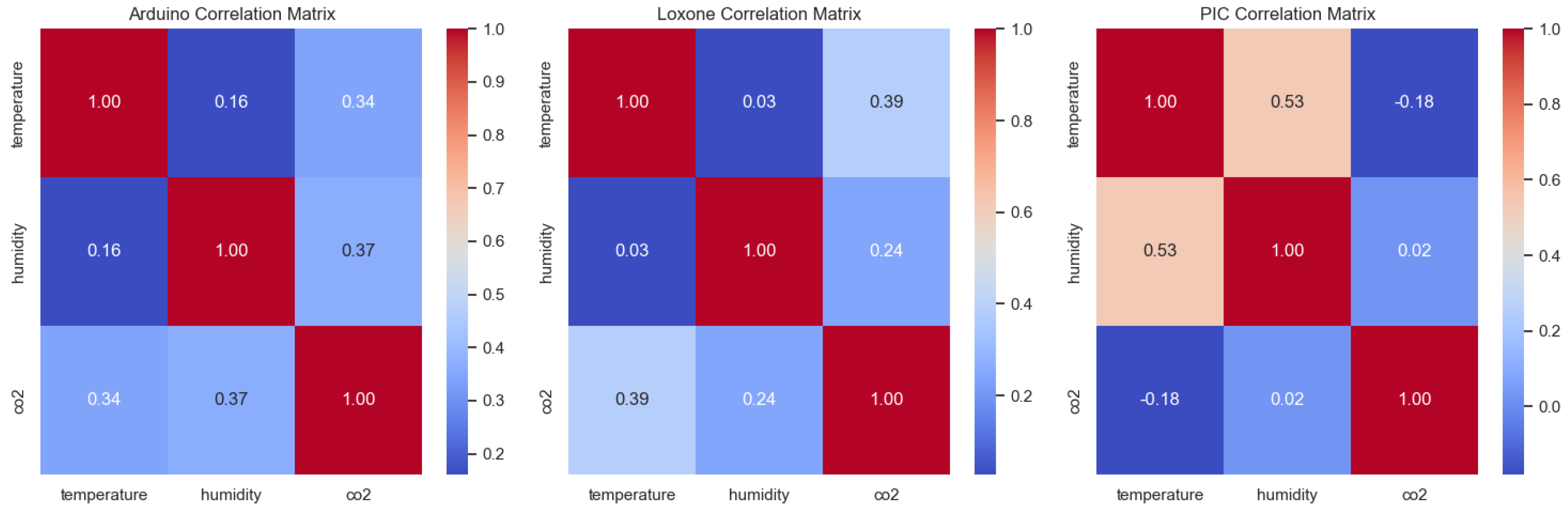
Figure 8.
Pair plot used to evaluate the relationships between environmental parameters (T, , ) relevant to trigger logic design.
Figure 8.
Pair plot used to evaluate the relationships between environmental parameters (T, , ) relevant to trigger logic design.
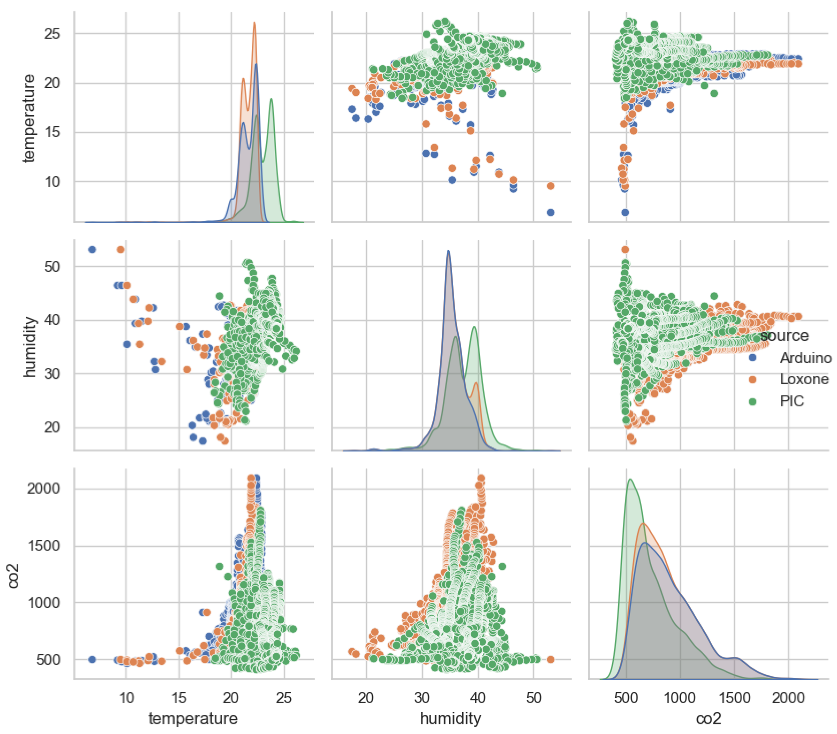
Figure 10.
F1 Score Heatmap for Trigger Thresholds.
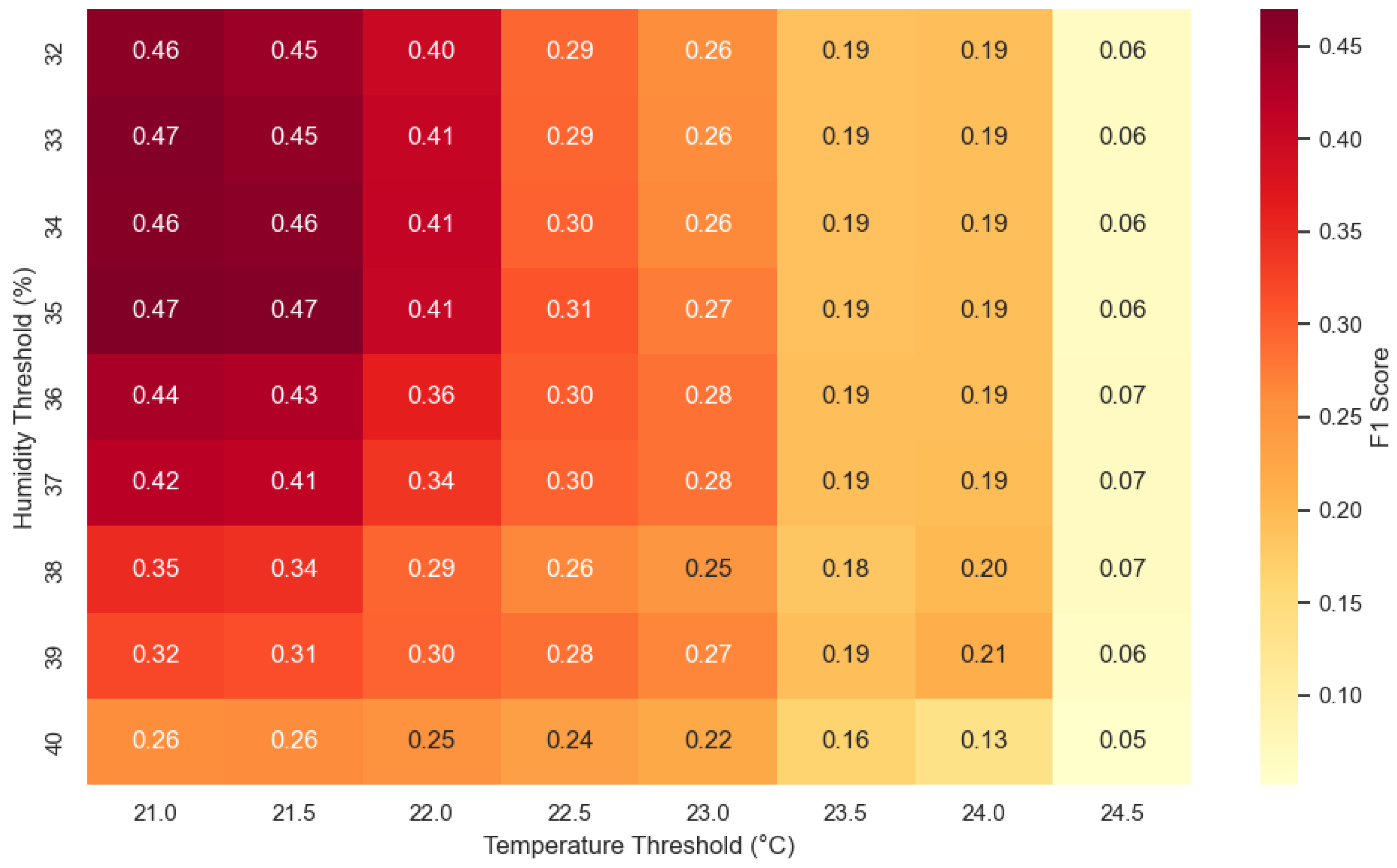
Figure 11.
Activation of measurements based on threshold exceedance of temperature and humidity.
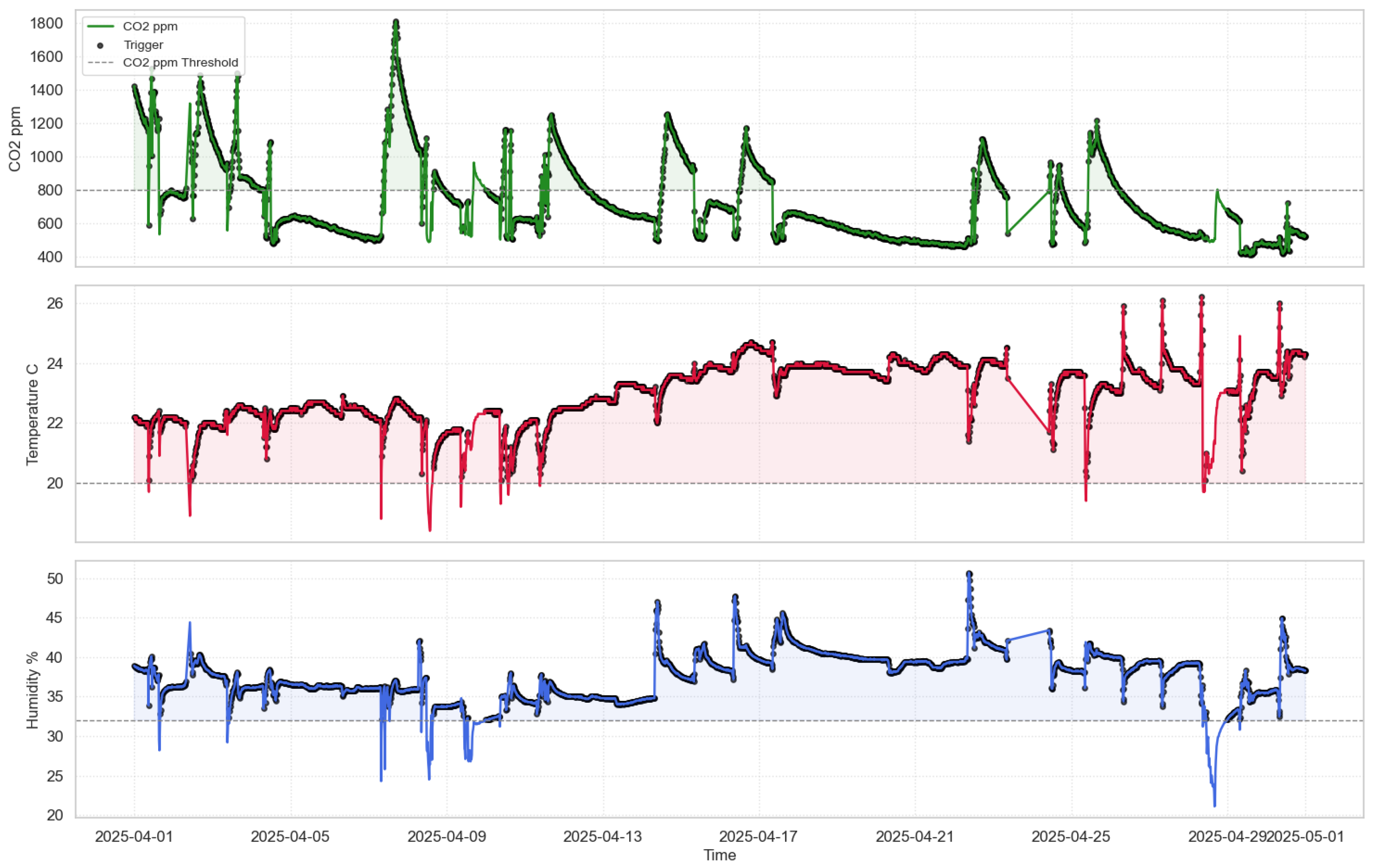
Figure 12.
Reconstructed signals from reduced measurement points using the proposed threshold-based sampling method.
Figure 12.
Reconstructed signals from reduced measurement points using the proposed threshold-based sampling method.
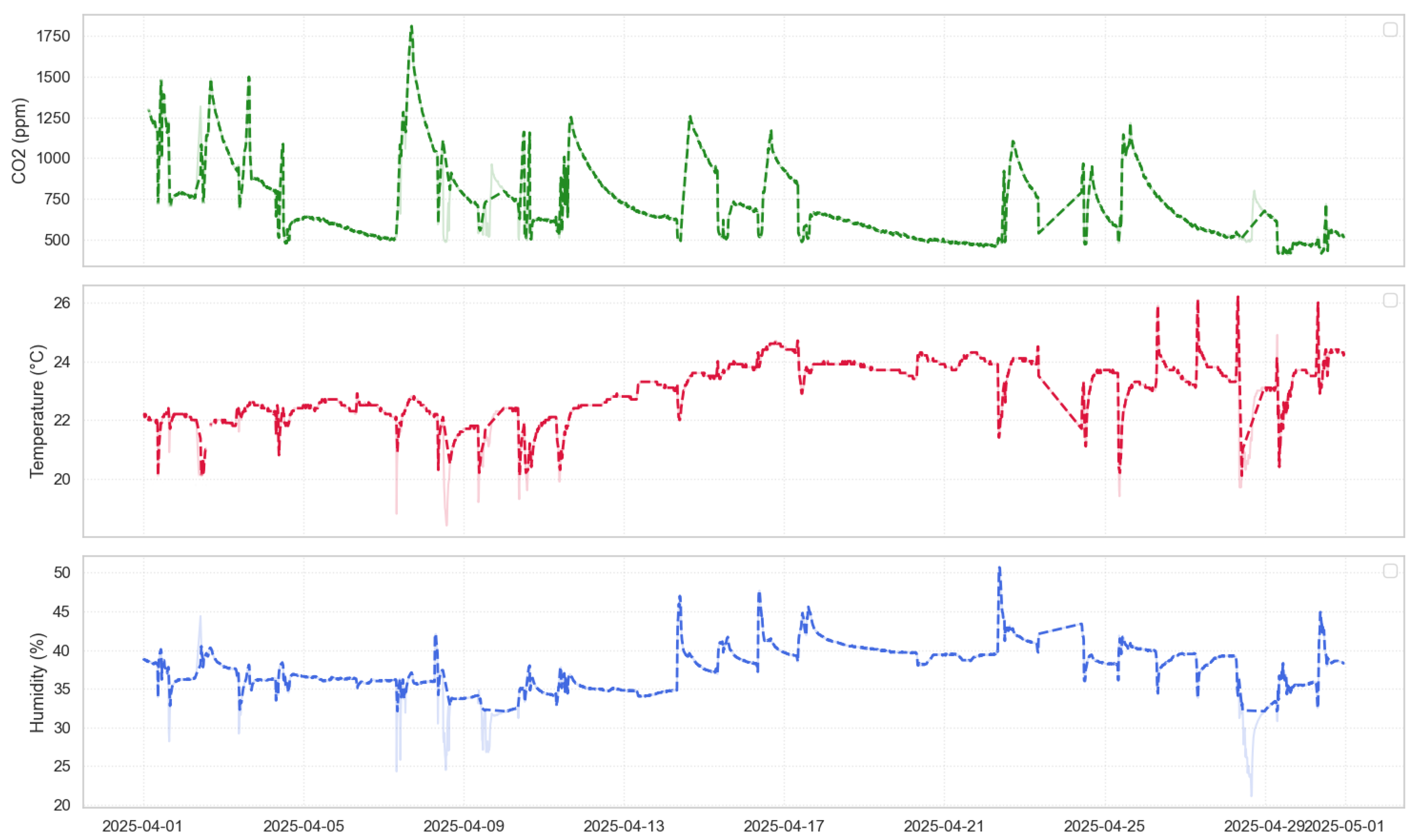

Table 1.
Data Reduction Methods.
| Method | Description | Reduced | MAE |
|---|---|---|---|
| RDP [12] | Keeps only the key points that form the waveform. | 68% | 0.0091 |
| PAA [22] | Reduces the signal dimension by dividing it into segments of equal length. | 62% | 0.0103 |
| vSAX [23] | Converts PAA values to discrete characters. | 65% | 0.0125 |
| Wavelet Tr. [25] | Decomposes a signal into components and removes small signal coefficients. | 70% | 0.0082 |
| Kalman Filter [24] | Smoothes and reduces noise | 60% | 0.0069 |
| Compressive Sensing [28] | Reconstructs signals from fewer samples. | 72% | 0.0073 |
| Delta Encoding [] | Reduces the redundancy of similar values | 50% | 0.0132 |
| Peak-to-Peak [26] | Keeps only significant peaks and valleys of the signal. | 59% | 0.0108 |
| Entropy-Based [29] | Preserves those signal segments with high information content. | 64% | 0.0099 |
| Variance-Based [27] | Compresses data to a value exceeding the threshold. | 61% | 0.0106 |
Table 2.
Top 5 threshold combinations for CO2 trigger (Sensor 1).
| T thresh. (°C) | H thresh. (%) | Precision | Recall | F1 | Trigger % |
|---|---|---|---|---|---|
| 20.5 | 31 | 0.311 | 0.990 | 0.473 | 95.4 |
| 20.0 | 31 | 0.310 | 0.996 | 0.473 | 96.3 |
| 20.5 | 35 | 0.329 | 0.842 | 0.473 | 76.8 |
| 20.0 | 35 | 0.328 | 0.847 | 0.473 | 77.3 |
| 19.5 | 35 | 0.327 | 0.848 | 0.472 | 77.6 |
Table 3.
Overview of Signal Reduction and Reconstruction Accuracy.
| Method | Description | Reduced (%) | MAE | RMSE |
|---|---|---|---|---|
| 2 to 1 | CO2 active, if T > 20.5 °C and H > 31% | 41.9% | 0.0089 | 0.0117 |
Disclaimer/Publisher’s Note: The statements, opinions and data contained in all publications are solely those of the individual author(s) and contributor(s) and not of MDPI and/or the editor(s). MDPI and/or the editor(s) disclaim responsibility for any injury to people or property resulting from any ideas, methods, instructions or products referred to in the content. |
© 2025 by the authors. Licensee MDPI, Basel, Switzerland. This article is an open access article distributed under the terms and conditions of the Creative Commons Attribution (CC BY) license (http://creativecommons.org/licenses/by/4.0/).
Copyright: This open access article is published under a Creative Commons CC BY 4.0 license, which permit the free download, distribution, and reuse, provided that the author and preprint are cited in any reuse.


