Submitted:
17 May 2025
Posted:
19 May 2025
You are already at the latest version
Abstract
Time-sensitive applications require the End-to-End (E2E) delay of wireless networks to be deterministic. For example, control signals in industrial automation, intelligent transportation, and telemedicine must be transmitted to their destinations within the millisecond range, with delay jitter controlled within the microsecond range. To formulate effective policies for maintaining E2E delay within a small deterministic range, it is essential to estimate the probability density function (PDF) of E2E delay. Data-driven methods based on mixture density networks have been employed to estimate the PDF of E2E delay in wireless networks. However, in WiFi networks, the estimation results produced by existing methods exhibit significant discrepancies and fluctuations when compared to actual measurements. Motivated by this, an improved estimation method is proposed, where the delay PDF is divided into three segments with different functional expressions that are coupled together. Moreover, the parameter estimation process is implemented in two stages. First, the two division thresholds for the three segments of the PDF are calculated based on the variation trend of E2E delay measurements. Second, the remaining parameters are obtained through training using an improved mixture density network. Experimental results indicate that the E2E delay PDF obtained by the proposed method exhibits a smaller gap compared to actual measurements than existing methods. Specifically, the mean absolute errors and average fluctuation amplitudes of tail probabilities at certain delay values decrease by at least one order of magnitude. Moreover, the multiple-segmentation feature of the proposed method enhances its robustness in situations where measurement data are affected by low levels of Gaussian noise.
Keywords:
Deterministic wireless network
; end-to-end delay
; mixture density network
; time-sensitive network
1. Introduction
Advancements in communication, computation, and artificial intelligence continuously promote the development of time-sensitive applications [1], such as industrial automation, intelligent transportation, telemedicine, data center networking, etc. Time-sensitive applications demand that the End-to-End (E2E) transmission delay remains within the millisecond range and that the delay jitter stays within the microsecond range, both with a high probability [2,3,4]. As depicted in Figure 1, for Ethernet, Time-Sensitive Networking (TSN) technology employs traffic shaping mechanisms such as IEEE 802.1Qav and IEEE 802.1Qbv to allocate deterministic transmission slots for high-priority traffic. This ensures the availability of transmission bandwidth and precise timing for critical operations, thereby enhancing the reliability and delay determinism of key services [5]. However, in wireless networks, factors such as dynamic node behavior, energy limitations, and perpetually evolving environments pose significant challenges to the implementation of TSN technologies. 5G ultra-reliable low-latency communication (URLLC) technology has achieved remarkable progress in reducing E2E delay. However, it does not adequately account for queueing delay, which may still pose challenges in certain real-time applications. As a result, there remains a gap in meeting the stringent delay requirements of time-sensitive applications. Consequently, ensuring a deterministic E2E delay remains a critical objective in the field of wireless networks. To achieve deterministic control of E2E delay in wireless networks, accurate delay estimation is essential, as relying solely on average delay is insufficient. Therefore, the delay probability density function (PDF) must be estimated so that resource and queue management strategies can be adjusted accordingly. This ensures the timely transmission of critical data even as network conditions change.
In the future, WiFi 7 is expected to incorporate TSN capabilities, thereby enabling ultra-reliability and low-latency in unlicensed frequency bands [2]. In contrast to mobile networks, the WiFi environment is predominantly indoor-oriented. Consequently, delay fluctuations in WiFi networks are less pronounced compared to those in mobile networks. Therefore, the estimation of the E2E delay PDF in WiFi networks is not as complex as that in mobile networks, yet similarities exist. In this paper, the primary focus is on the estimation of the E2E delay PDF in WiFi networks. It is expected that the associated findings can be extended and applied to mobile networks. At present, the estimation methods for network delay PDFs can be categorized into two types: theoretical analysis approaches and data-driven methods. Theoretical analysis methods generally depend on a set of assumptions and utilize mathematical tools to solve and analyze the system behavior. However, these assumptions may not always align with practical scenarios. In recent years, the integration of machine learning into network delay estimation has garnered significant attention [6]. The development in this field is primarily driven by data-driven approaches, where machine learning techniques based on neural networks are utilized to identify and learn the relationships between delay and other variables by extracting insights from real-world data.
As a representative data-driven approach, Mixture Density Networks (MDNs) have been extensively applied and validated for delay PDF estimation in complex systems. MDNs integrate neural networks with probabilistic models, such as the Gaussian Mixture Model (GMM), to estimate the parameters of the mixture model via a fully connected neural network, thereby generating a conditional PDF. Recently, Mostafavi et al. [7] employed MDN in conjunction with the Generalized Pareto Distribution (GPD) to estimate the E2E delay PDF of several real networks, including Commercial Off-The-Shelf (COTS) 5G, Open Air Interface (OAI) 5G, and Mango COMM IEEE 802.11 (WiFi). MDN maps the transmission conditions or traffic characteristics to the parameters of the PDF and generates the PDF. However, for WiFi networks, there is a noticeable gap between the estimation results and actual measurements, particularly in the tail of the PDF. To address this issue, this paper proposes a two-stage and three-divided estimation method, referred to as TSTD, for estimating the E2E delay PDF in WiFi networks. The main contributions are summarized as follows.
- A three-divided PDF is constructed, consisting of a main part and a two-segment tail part. The main part is modeled using GMM, while the two segments of the tail part are modeled using distinct GPDs. Additionally, the coupling relationships between the different segments in the main part and the tail part are taken into account.
- For the parameters of the PDF, the thresholds of the GPDs are determined based on the variation trend of the tail probability in E2E delay measurements, and the remaining parameters are obtained through training via MDN.
- Compared with existing methods, the E2E delay PDF obtained using the proposed method exhibits a smaller discrepancy from actual measurements. In particular, the mean absolute errors and average fluctuation amplitudes of tail probabilities at certain delay values are reduced by at least one order of magnitude. Moreover, the multiple-segmentation feature of the proposed method enhances its robustness in situations where measurement data are affected by low levels of Gaussian noise.
The remainder of this paper is structured as follows. Section 2 reviews the related work. Section 3 provides a concise introduction to the research problem. Section 4 elaborates on the proposed two-stage and three-divided estimation method. Section 5 details the experimental procedures and performance analysis. Finally, Section 6 presents the conclusion and discusses future work.
2. Related Work
The estimation methods for the E2E delay probability distribution in multiple application scenarios have garnered significant attention. Cao et al. [8] modeled the Mobile Edge Computing (MEC) network as a two-stage tandem queueing system. Subsequently, they proposed an estimation method for the probability distribution of the E2E delay using the matrix-geometric method. Mei et al. [9] modeled and analyzed the delay bound of a multi-cluster MEC network using the stochastic network calculus (SNC) approach. Cui et al. [10] proposed a method for calculating the E2E delay violation probability of target traffic in the industrial Internet of Things (IoT), also based on SNC. Coll-Perales et al. [11] proposed a 5G E2E delay model for Vehicle-to-Network (V2N) and Vehicle-to-Network-to-Vehicle (V2NV2N) communications. They quantified and analyzed the 5G E2E delay performance for V2N and V2NV2N communications under various 5G network deployments and configurations.
The aforementioned methods are all theoretical analysis. Theoretical analysis methods generally rely on a series of assumptions and employ mathematical tools to solve and analyze the system’s behavior. However, these assumptions may not always align with practical scenarios. In view of this, data-driven methods have been extensively studied for estimating network delay probability distributions.
Fadhil et al. [12] proposed a method for modeling the E2E delay of 5G networks using a GMM. Based on E2E delay data, an Expectation-Maximization (EM) algorithm was employed to estimate the GMM parameters. The results indicate that as the number of data samples and GMM components increases, higher accuracy can be achieved. However, the computation time also increases rapidly with the increase in the number of samples and components. Specifically, the increasing trend is approximated as an exponential behavior as the number of GMM components increases [12]. In [13], Chen et al. employed the deep learning approach to generate the probability density function (PDF) of practical data. The cumulative distribution functions (CDFs) of common probability distributions were utilized as activation functions in the hidden layers of the proposed deep learning model to learn actual cumulative probabilities. Furthermore, the differential equation derived from the trained deep learning model can be used to estimate the PDF. Experimental results demonstrated that both the CDF and PDF can be accurately estimated by the proposed method, as assessed by the mean absolute percentage error. In [14], the MDN combined with GMM was utilized to estimate the delay probability distribution of single-stage queueing systems. Subsequently, this work was extended by Raeis et al. [15] to more complex systems, namely service function chains. In [14,15], the estimation methods have been proven effective in fitting the main part of the delay probability distribution using machine learning techniques. However, the fitting results for the tail part of the distribution are less satisfactory. This is because the output of GMM-based models typically exhibits exponentially decaying tail probabilities, which can lead to significant errors when dealing with low-probability events, especially in the case of heavy-tailed distributions.
It is shown in some literature that better fitting results can be obtained when the main and tail parts of the delay probability distribution are fitted using different functions respectively. Yasuda et al. [16] utilized the bistate model to simulate wireless networks involving connection and disconnection processes. For the E2E delay probability distribution, the main part, which arises during the connection process, was fitted using the shifted Gamma distribution. In contrast, the tail part, resulting from the accumulation of probe packets during the disconnection phase, was approximated by the exponential distribution. This approach exhibited superior performance compared to traditional methods in terms of both the negative log predictive density (NLPD) [17] and the continuous ranked probability score (CRPS) [18]. In addition, the GPD is a classical asymptotically motivated model for the unknown excess distribution above high thresholds [19,20]. Consequently, it has been widely applied to fit the tail part of the delay PDF [7,21]. In [21], Mostafavi et al. proposed an extreme value mixture model based on the mixture density network (MDN). This was achieved by integrating the GPD tail model with the GMM. Specifically, the GMM was used to capture the main part of the delay PDF, while the GPD was employed to characterize the tail of the delay PDF. Numerical experiments conducted on a three-stage tandem queueing system demonstrated that the proposed method outperforms existing state-of-the-art GMM-based estimation techniques. Furthermore, Mostafavi et al. [7] integrated the MDN with the GPD to estimate the PDF of E2E delay in three wireless network scenarios, namely commercial off-the-shelf (COTS) 5G, Open Air Interface (OAI) 5G, and Mango COMM IEEE 802.11 (WiFi). The GMM was employed to fit the main part of the delay probability distribution, while the tail part was modeled using the GPD. For the 5G scenarios, this approach exhibited robust performance through noise regularization when the tail profile was nonsmooth. However, in the WiFi network scenario, the estimation results showed a significant gap and fluctuation compared to actual measurements.
In [7], the threshold parameter of the GPD is obtained through training. It is worth noting that the threshold parameter of the GPD can also be determined using other methods, such as empirical approaches and graphical techniques. The empirical method depends on an analyst’s statistical knowledge and expertise to select an appropriate threshold, which may introduce bias [22,23]. Graphical diagnostic methods [24] have been widely used for threshold estimation, utilizing specific plots of the measured data to observe trends and assist in threshold selection. Cyrille et al. [25] utilized graphical diagnostic tools to determine the threshold range. Based on this, they established specific thresholds and optimized the parameters of the GPD using the Kolmogorov-Smirnov (KS) goodness-of-fit test. They further validated that the estimated parameters exhibited improved accuracy with larger sample sizes through the use of actual hydrological data. Zhao et al. [26] pointed out that the process of GPD parameter estimation is independent of threshold selection. They compared the performance of three threshold selection procedures to determine an appropriate threshold for asymptotic fitting of the GPD above this threshold. The results demonstrated that this estimator achieved satisfactory performance in environmental data analysis, particularly in fitting the tail probability distribution.
Drawing on the strengths of the existing works mentioned above, this paper proposes an improved estimation method to enhance the accuracy of fitting the E2E delay PDF in WiFi networks. Firstly, the threshold parameter of the GPD is determined based on the variation trend of E2E delay measurements. Subsequently, the remaining parameters of the GPD are estimated via the MDN. Moreover, the tail part of the delay PDF is divided into two segments, each of which is fitted using a distinct GPD.
3. Research Problem Statement
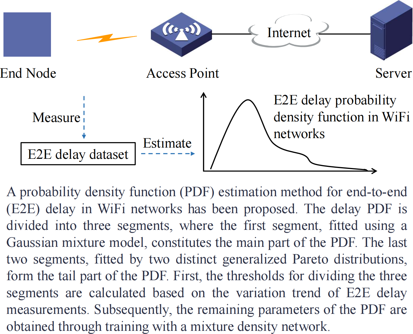
The conditional PDF for the E2E delay Y of packets with length X in WiFi networks is estimated based on the measured delay data, as illustrated in Figure 2.
Let denote the delay dataset measured over a period of time, where is the record corresponding to the n-th packet, denotes the packet length, , , and denotes the E2E (uplink or downlink) delay. For packets with length , the conditional PDF will be estimated using some samples from the delay dataset, where represents the estimated parameter vector. In additional, the CDF is denoted as . The tail probability is denoted as .
4. Two-Stage and Three-Divided Estimation Method
The proposed method, TSTD, consists of two steps: namely, PDF construction and parameter estimation, as described below.
4.1. PDF construction
The PDF is expressed in the form of (1), where
comprises both the main part and the tail part, with the latter being further divided into two segments, as illustrated in Figure 3.
4.1.1. Main part
The segment within the range of is modeled using the GMM, and its PDF is represented as .
where
represents the Gaussian PDF with mean and standard deviation , where denotes the weight. The corresponding CDF is expressed as .
4.1.2. Tail part
For the segment within the range of , the PDF is a mixture of and , as given by the second formula in (1). For the segment within the range of , the PDF is a mixture of and , , as described by the third formula in (1). Here, represents the mixture weight, and denotes the PDF of GPD, as defined in (5).
where
. when , and when . The corresponding CDF is expressed as , .
The motivations for dividing the tail part into two segments and considering the coupling relationship between different segments are as follows. The variation trend of the tail probability distribution of the measured delay indicates that the tail initially decreases slowly. However, as the delay exceeds a certain threshold, the tail probability begins to fluctuate and subsequently decreases at a faster rate. Although the GPD exhibits heavy-tailed characteristics, a single GPD is insufficient to capture the variation characteristics of the tail probability. Therefore, the tail part is divided into two segments, each of which is fitted using distinct GPDs. Additionally, according to the reference [13], fitting the probability distribution of actual data using a mixture of multiple probability distributions yields good results. Hence, the coupling relationship between the segments fitted by the GMM and GPDs is considered.
4.2. Parameter estimation for PDF
For the PDF , the parameter vector is estimated in two stages, as illustrated in Figure 4. In the first stage, the thresholds and in and are determined. In the second stage, the remaining parameters, which constitute the parameter vector , are estimated via MDN.
4.2.1. First stage: Determine the thresholds and .
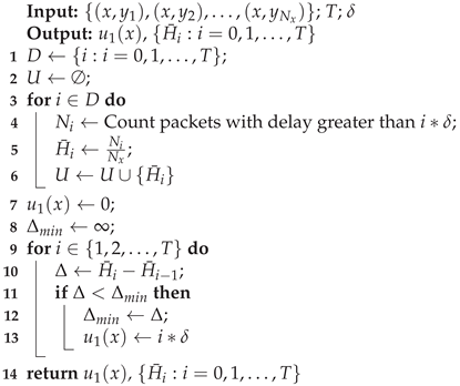
The threshold is utilized to divide the main and tail parts of the delay PDF under the condition of packet length x. Based on the characteristics of heavy-tailed distributions, significant fluctuations typically occur around the inflection point between the main and tail parts. Consequently, is defined as the delay value at which the absolute value of the differential tail probability attains its maximum. It is computed according to Algorithm 1. The inputs include the delay dataset for packets with length x, , the size of the tail probability sequence, and the interval between adjacent delays in the tail probability sequence, such as ms. The outputs are the threshold and the tail probability sequence .
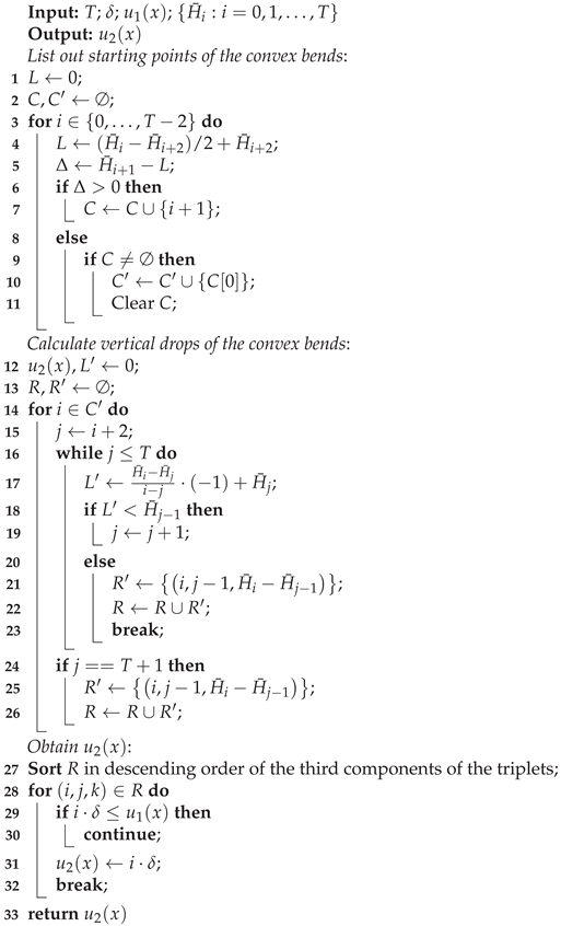
The threshold is utilized to divide the tail part into two segments. Analysis of the measured delay dataset reveals that the tail initially decreases slowly and subsequently exhibits a faster rate of decrease. This transition occurs at a convex bend. Consequently, is defined as the delay value corresponding to the starting point of the convex bend with the maximum vertical drop, as illustrated in Figure 5. It is determined through Algorithm 2, with inputs including T, , , and the tail probability sequence .
| Algorithm 1: Calculate threshold |
 |
Algorithm 2 comprises three steps. In the first step, the starting points of the convex bends in the tail probability sequence are identified in lines 1-11 of Algorithm 2, and these points are also referred to as the starting points of convex point clusters. A convex point cluster is defined as a group of consecutive convex points. The point , , is termed a convex point if the following relationship (8) is satisfied.
In the second step, the convex bends in the tail probability sequence are identified, and their vertical drops are subsequently calculated in lines 12-26 of Algorithm 2. A set of consecutive convex points form a convex bend if the following relationship (9) is satisfied for all .
The vertical drop of the aforementioned convex bend is computed as .
In the third step, is determined in lines 27-33 of Algorithm 2. Specifically, corresponds to the starting point of the convex bend with the maximum vertical drop located on the right side of .
4.2.2. Second stage: Train the remaining parameters.
The parameter vector is estimated using a MDN, which comprises one input layer, four hidden layers, one output layer, and one custom layer, as illustrated in Figure 4. The custom layer is utilized to set the thresholds obtained in the first stage. The output layer consists neurons that output the parameters in . The input layer contains a single neuron, into which the packet lengths from the dataset are fed in batches with batch size during each epoch. Additionally, the delays are used in the loss function NLPD [17], which is defined as follows.
where and . Moreover, the training process is carried out in multiple rounds with varying learning rates, and each round is divided into several epochs.
| Algorithm 2: Calculate threshold |
 |
The aforementioned training process is adapted from reference [7]. Unlike [7], the PDF in this paper comprises a main part and a two-segment tail part. The two segments of the tail part are modeled using distinct GPDs, with consideration given to the coupling relationship between segments. The thresholds for dividing the three segments are determined based on the variation trend of tail probabilities derived from historical measured delay data, rather than through training. Meanwhile, the remaining parameters are estimated via MDN-based training.
Remark 1: The loss function NLPD is essentially a negative log-likelihood. Our objective is to minimize the negative log-likelihood, which is equivalent to performing maximum likelihood estimation (MLE). However, when the classical approach for maximizing the likelihood is applied to estimate the parameters of the delay PDF, it demonstrates poor scalability. This limitation arises from the necessity of inverting a large number of covariance matrices proportional to the number of data points [27]. In contrast, an effective alternative is the deep learning framework, which utilizes the NLPD as the loss function.
5. Experiments on WiFi Networks
In this section, we compare the proposed method TSTD with existing approaches in terms of their accuracy in estimating the delay PDF. The subsequent subsections provide a detailed description of the experimental procedures, including data preprocessing, threshold determination, model training, and performance evaluation.
5.1. Data Preprocessing
Four datasets provided by Mostafavi et al. [7] are utilized, corresponding to four types of packets with varying lengths (172 bytes, 3440 bytes, 6880 bytes, and 10320 bytes). Each dataset comprises over one million samples that record the packet length and downlink delay in software-defined radio (SDR) WiFi networks. The data collection environment for the SDR WiFi networks consists of a conference room measuring 50 m2, equipped with metallic chairs, whiteboards, and screens. For collecting data related to packets with a length of 172 bytes, the coordinate of the end node location is set variably at and within a coordinate system (with scale units in meters) using the access point as the origin. This can simulate the small-scale movement of the end node. For other packet types, the end node location is consistently set at . The packet generation interval was established at 10 ms. Basic information regarding the utilized datasets is presented in Table 1.
The datasets undergo preprocessing in accordance with the following steps. First, the datasets are normalized by scaling the delay values to the millisecond level. Then, standardization is performed by subtracting the mean from the normalized delay values, yielding zero-mean delay values, to avoid training errors caused by dataset biases. Finally, to enhance the convergence speed during training, the four types of packet lengths are normalized by scaling them to the range .
5.2. Threshold Determination
The first stage illustrated in Figure 4 is carried out, where Algorithms 1 and 2 are employed to compute the thresholds and for packets with lengths 172, 3440, 6880, and 10320 bytes, respectively. The input dataset for the algorithms takes the form , where represents the delay values scaled to the millisecond level. Additionally, the other two inputs for each packet type are set as and . For each packet length, the computed threshold values are shown in Table 2.
5.3. Model Training
The second stage illustrated in Figure 4 is carried out, where the parameter vector is obtained by training the MDN model. In this model, the number of Gaussian distributions in (3) is set to . The first to fourth hidden layers contain 10, 50, 50, and 40 neurons, respectively. The activation function for each neuron is set to the ’tanh’ function. For the output layer, the neurons corresponding to have no activation function, while the neurons corresponding to use ’softmax’ functions. The remaining neurons employ ’softplus’ functions as their activation functions. For the custom layer, the parameters and are fixed at the values calculated in Section 5-5.2.
The training dataset, in the form of is utilized, where and represent the normalized packet length and delay value, respectively. This training dataset is constructed through three steps. First, the four datasets corresponding to different packet lengths are merged into a single dataset. Then, the samples in the merged dataset are randomly shuffled. Finally, N samples are randomly sampled from the shuffled dataset according to a specified sampling ratio, forming the training dataset.
The training process is carried out in four rounds with learning rates of , , , and , respectively. Each round consists of 200 epochs. In each epoch, the batch size is set to of the number of samples in the training dataset.
5.4. Performance Evaluation
The performance of TSTD is evaluated in terms of the means and fluctuation amplitudes of the delay tail probabilities, and it is compared with two existing methods. One method is GMM [15], which is one of the state-of-the-art approaches for probability density estimation. The other method is GMEVM [7], which integrates GPD with GMM.
First, Q training datasets are independently sampled with a sampling ratio of , and these datasets are used to train and obtain Q PDFs. In the experiment, Q was set to 9. The mean and fluctuation amplitude of Q tail probability distributions are plotted in Figure 6, where the delay value serves as the abscissa and the common logarithm of the tail probability serves as the ordinate. The solid line represents the mean, while the shaded area represents the fluctuation amplitude. It can be observed that both GMM and GMEVM exhibit larger deviations from the actual measurements (denoted as MEAS), whereas TSTD fluctuates around the actual measurements.
Then, similar to the above case, the experiment results for the sampling ratios and are presented in Figure 7 and Figure 8, respectively. It can be observed that the fluctuation amplitudes of both GMEVM and TSTD decrease as the sampling ratio of the training dataset increases. TSTD always follows the actual measurements as the delay increases, while GMEVM initially exhibits heavy-tail characteristics and gradually deviates from the actual measurements. Because a single GPD is insufficient for accurately capturing the probabilistic characteristics when the tail exhibits heavy-tailed behavior accompanied by fluctuations. Even though the sampling ratio increases to , GMM continues to exhibit significant fluctuations relative to the actual measurements. This is due to the fact that as the sampling ratio increases, the influence of tail events becomes more pronounced. Fitting heavy-tailed distributions using GMM introduces substantial errors given the inherent limitations of GMM. This issue persists even when the number of GMM components is increased, as shown in Figure 9, where the number of components is set to 20.
Next, the model is trained using the complete dataset. As shown in Figure 10, the improvement in estimation performance is not significant. In dynamic wireless environments, the model needs to be updated periodically. Introducing a data sampling strategy can effectively reduce computational costs. Thus, achieving an appropriate balance between the sampling ratio (or training time) and model performance is essential for efficient model updates. Table 3 provides a detailed summary of the average training time for Q PDFs under different sampling ratios. Adding one segment means that the model needs to train additional parameters, which also increases the training time to some extent. TSTD requires longer training time compared to GMM and GMEVM. However, the difference is not significant compared to GMEVM, especially when the size of the training dataset is larger.
Furthermore, the mean absolute error () and average fluctuation amplitude () of tail probabilities across all considered delays are utilized to evaluate the performance of estimation methods.
where represents the mean absolute error of tail probabilities at delay y, conditioned on packet length x, considering the Q PDFs estimated from Q training datasets.
. represents the tail probability at delay y given packet length x, estimated independently using the i-th training dataset, where . Additionally, denotes the measured tail probability at delay y under the condition of packet length x.
where represents the average fluctuation amplitude of tail probabilities at delay y given packet length x, considering Q PDFs estimated from Q independent training datasets.
and denote the functions used to select the maximum and minimum values, respectively, from a given set.
As shown in Table 4, for TSTD with a sampling ratio of , both and decrease compared to GMM and GMEVM.
For some delay values, the MAE and AFA of TSTD either remain at the same order of magnitude or decrease by at least one order of magnitude compared with GMM and GMEVM. For example, the MAEs and AFAs for certain delay values are listed in Table 5 and Table 6. However, for specific delay values, the MAE of TSTD increases by one order of magnitude compared to GMM, while the AFA decreases by one order of magnitude, with the fluctuation interval still lying within that of GMM. The PDFs constructed in GMM and TSTD are used to approximate the PDF of E2E delays. In this approximation process, the loss function is defined as the mean of negative log probability densities over multiple delays, which measures the average closeness between the estimated result and the target. Therefore, compared with GMM, it is possible for TSTD to exhibit poor fitting results on a small number of points, but its overall performance remains superior.
Finally, the potential inaccuracies or noise in delay measurements are considered as factors that could influence the estimation results. To evaluate the performance of estimation methods under such conditions, random Gaussian noises with variances of 1 ms and 3 ms are respectively introduced into the delay samples. As shown in Figure 11 and Figure 12, in the low-delay domain, as the noise variance increases, the mean of each method gradually deviates from the actual measurements, while their fluctuation amplitudes remain largely unaffected. In the high-delay domain, as the noise variance increases, the mean and fluctuation amplitude of TSTD remain almost unchanged. For GMEVM, its fluctuation amplitude initially increases and then decreases, while its mean remains nearly constant. For GMM, both its mean and fluctuation amplitude are relatively stable, with the latter continuing to decrease slightly. This is because a higher proportion of data lies in the low-delay domain, where changes in these data can significantly affect the mean of the fitting results. Additionally, the added noise tends to smooth out sharp fluctuations, ultimately reducing the fluctuation amplitudes. In summary, compared with GMM and GMEVM, the multiple-segmentation feature of TSTD makes it more robust when measurement data are slightly inaccurate or contain low levels of noise.
6. Conclusion and Future Work
In this paper, a PDF estimation method for the E2E delay in WiFi networks is proposed. The delay PDF is divided into three segments: the first segment, fitted by GMM, constitutes the main part of the PDF, while the last two segments, fitted by two different GPDs, constitute the tail part of the PDF. The thresholds for dividing the three segments are calculated first, and the other parameters of the PDF are subsequently obtained through training using MDN. Experimental validation demonstrates that this approach achieves results closer to measurement data compared to existing methods. Specifically, the mean absolute errors and average fluctuation amplitudes of tail probabilities at certain delay values decrease by at least one order of magnitude. Moreover, the multiple-segmentation feature of the proposed method enhances its robustness in situations where measurement data are affected by low levels of Gaussian noise.
In the future, further refinements will focus on integrating additional network parameters as conditioning variables to enhance both the model’s accuracy and adaptability. Potential parameters encompass modulation and coding scheme (MCS), packet arrival intervals, signal-to-noise ratio (SNR), and packet loss rate. Moreover, assessing the model’s generalizability beyond WiFi networks, such as in 5G and IoT networks, represents a critical research direction. Ultimately, the estimation results will provide a robust foundation for devising deterministic delay control strategies.
Author Contributions
Conceptualization, J.C. and Y.D.; methodology, J.C.; software, Y.D.; validation, J.C. and Y.D.; formal analysis, S.H.; investigation, S.H.; resources, M.Z.; data curation, M.Z.; writing—original draft preparation, Y.D.; writing—review and editing, J.C. All authors have read and agreed to the published version of the manuscript.
Funding
This work was supported in part by the National Natural Science Foundation of China under Grant 62361017, in part by Natural Science Foundation of Guangxi under Grant 2023GXNSFBA026212, in part by Research Foundation Ability Enhancement Project for Young and Middle aged Teachers in Guangxi Universities under Grant 2023KY0227, in part by the Open Project of State Key Laboratory of Public Big Data under Grant PBD2022-09, and in part by the Innovation Project of GUET Graduate Education 2025YCXS068.
Data Availability Statement
The original contributions presented in the study are included in the article, and further inquiries can be directed to the corresponding author.
Conflicts of Interest
The authors declare no conflicts of interest.
References
- Qiao, Y.; Niu, Y.; Chen, S.; Zhong, Z.; Zhang, C.; Wang, N.; Ai, B. Energy Efficiency Optimization of Ultra-Reliable Low-Latency Communication for High-Speed Rail. IEEE Transactions on Vehicular Technology 2024, 73, 16638–16653. [Google Scholar] [CrossRef]
- Adame, T.; Carrascosa-Zamacois, M.; Bellalta, B. Time-Sensitive Networking in IEEE 802.11be: On the Way to Low-Latency WiFi 7. Sensors 2021, 21. [Google Scholar] [CrossRef] [PubMed]
- Lee, H.; Choi, Y.; Han, T.; Kim, K. Probabilistically Guaranteeing End-to-End Latencies in Autonomous Vehicle Computing Systems. IEEE Transactions on Computers 2022, 71, 3361–3374. [Google Scholar] [CrossRef]
- Han, F.; Wang, M.; Cui, Y.; Li, Q.; Liang, R.; Liu, Y.; Jiang, Y. Future Data Center Networking: From Low Latency to Deterministic Latency. IEEE Network 2022, 36, 52–58. [Google Scholar] [CrossRef]
- Finn, N. Introduction to Time-Sensitive Networking. IEEE Communications Standards Magazine 2018, 2, 22–28. [Google Scholar] [CrossRef]
- Flinta, C.; Yan, W.; Johnsson, A. Predicting Round-Trip Time Distributions in IoT Systems using Histogram Estimators. In Proceedings of the NOMS 2020 - 2020 IEEE/IFIP Network Operations and Management Symposium, IEEE, Budapest, Hungary, 20-24 Apr. 2020; pp. 1–9. [Google Scholar]
- Mostafavi, S.; Sharma, G.P.; Gross, J. Data-Driven Latency Probability Prediction for Wireless Networks: Focusing on Tail Probabilities. In Proceedings of the GLOBECOM 2023 - 2023 IEEE Global Communications Conference, IEEE, Kuala Lumpur, Malaysia, 04-08 Dec. 2023; pp. 4338–4344. [Google Scholar]
- Cao, J.; Feng, W.; Ge, N.; Lu, J. Delay Characterization of Mobile-Edge Computing for 6G Time-Sensitive Services. IEEE Internet of Things Journal 2021, 8, 3758–3773. [Google Scholar] [CrossRef]
- Mei, M.; Yao, M.; Yang, Q.; Qin, M.; Kwak, K.S.; Rao, R.R. Delay Analysis of Mobile Edge Computing Using Poisson Cluster Process Modeling: A Stochastic Network Calculus Perspective. IEEE Transactions on Communications 2022, 70, 2532–2546. [Google Scholar] [CrossRef]
- Cui, P.; Han, S.; Xu, X.; Zhang, J.; Zhang, P.; Ren, S. End-to-End Delay Performance Analysis of Industrial Internet of Things: A Stochastic Network Calculus Perspective. IEEE Internet of Things Journal 2024, 11, 5374–5387. [Google Scholar] [CrossRef]
- Coll-Perales, B.; Lucas-Estañ, M.C.; Shimizu, T.; Gozalvez, J.; Higuchi, T.; Avedisov, S.; Altintas, O.; Sepulcre, M. End-to-End V2X Latency Modeling and Analysis in 5G Networks. IEEE Transactions on Vehicular Technology 2023, 72, 5094–5109. [Google Scholar] [CrossRef]
- Fadhil, D.; Oliveira, R. Estimation of 5G Core and RAN End-to-End Delay through Gaussian Mixture Models. Computers 2022, 11. [Google Scholar] [CrossRef]
- Chen, C.H.; Song, F.; Hwang, F.J.; Wu, L. A Probability Density Function Generator Based on Neural Networks. Physica A: Statistical Mechanics and its Applications 2020, 541. [Google Scholar] [CrossRef]
- Raeis, M.; Tizghadam, A.; Leon-Garcia, A. Predicting Distributions of Waiting Times in Customer Service Systems using Mixture Density Networks. In Proceedings of the 2019 15th International Conference on Network and Service Management (CNSM), IEEE, Halifax, NS, Canada, 21-25 Oct. 2019; pp. 1–6. [Google Scholar]
- Raeis, M.; Tizghadam, A.; Leon-Garcia, A. Probabilistic Bounds on the End-to-End Delay of Service Function Chains using Deep MDN. In Proceedings of the 2020 IEEE 31st Annual International Symposium on Personal, Indoor and Mobile Radio Communications, IEEE, London, UK, 31 Aug.-03 Sep. 2020; pp. 1–6. [Google Scholar]
- Yasuda, S.; Yoshida, H. Prediction of Round Trip Delay for Wireless Networks by a Two-state Model. In Proceedings of the 2018 IEEE Wireless Communications and Networking Conference (WCNC), IEEE, Barcelona, Spain, 15-18 Apr. 2018; pp. 1–6. [Google Scholar]
- Good, I.J. Rational Decisions. Journal of the Royal Statistical Society: Series B (Methodological) 1952, 14, 107–114. [Google Scholar] [CrossRef]
- Gneiting, T.; Raftery, A.E. Strictly Proper Scoring Rules, Prediction, and Estimation. Journal of the American Statistical Association 2007, 102, 359–378. [Google Scholar] [CrossRef]
- Scarrott, C.; MacDonald, A. A Review of Extreme Value Threshold Estimation and Uncertainty Quantification. REVSTAT-Statistical Journal 2012, 10, 33–60. [Google Scholar]
- Gomes, M.I.; Guillou, A. Extreme Value Theory and Statistics of Univariate Extremes: A Review. International Statistical Review 2015, 83, 263–292. [Google Scholar] [CrossRef]
- Mostafavi, S.S.; Dán, G.; Gross, J. Data-Driven End-to-End Delay Violation Probability Prediction with Extreme Value Mixture Models. In Proceedings of the 2021 IEEE/ACM Symposium on Edge Computing (SEC), IEEE, San Jose, CA, USA, 14-17 Dec. 2021; pp. 416–422. [Google Scholar]
- DuMouchel, W.H. Estimating the Stable Index α in Order to Measure Tail Thickness: A Critique. The Annals of Statistics 1983, 11, 1019–1031. [Google Scholar] [CrossRef]
- Ferreira, A.; de Haan, L.; Peng, L. On Optimising the Estimation of High Quantiles of a Probability Distribution. Statistics 2003, 37, 401–434. [Google Scholar] [CrossRef]
- Alaswed, H. Graphical Diagnostics for Threshold Selection in Fitting the Generalized Pareto Distribution. Journal of Pure & Applied Sciences 2024, 23, 90–95. [Google Scholar]
- Cyrille, O.G.; Keita, K. Machine Learning Method to Estimate Parameters of the GPD Distribution: Applied to Lobo Flows and Yzeron Water Levels. Mathematical Geoscience 2024. [Google Scholar] [CrossRef]
- Zhao, X.; Zhang, Z.; Cheng, W.; Zhang, P. A New Parameter Estimator for the Generalized Pareto Distribution under the Peaks over Threshold Framework. Mathematics 2019. [Google Scholar] [CrossRef]
- Lin, A.; Tolooshams, B.; Atchadé, Y.; Ba, D. Probabilistic Unrolling: Scalable, Inverse-Free Maximum Likelihood Estimation for Latent Gaussian Models. In Proceedings of the The Fortieth International Conference on Machine Learning (ICML), Honolulu, Hawaii, USA, 27 Jul. 2023; pp. 1–29. [Google Scholar]
- Mostafavi, S. SDR WiFi Measurement Commands. https://github.com/samiemostafavi/wireless-pr3d/blob/main/measurements/campaign1/IEEE80211g.md.
Figure 1.
Deterministic delay network for time-sensitive applications.
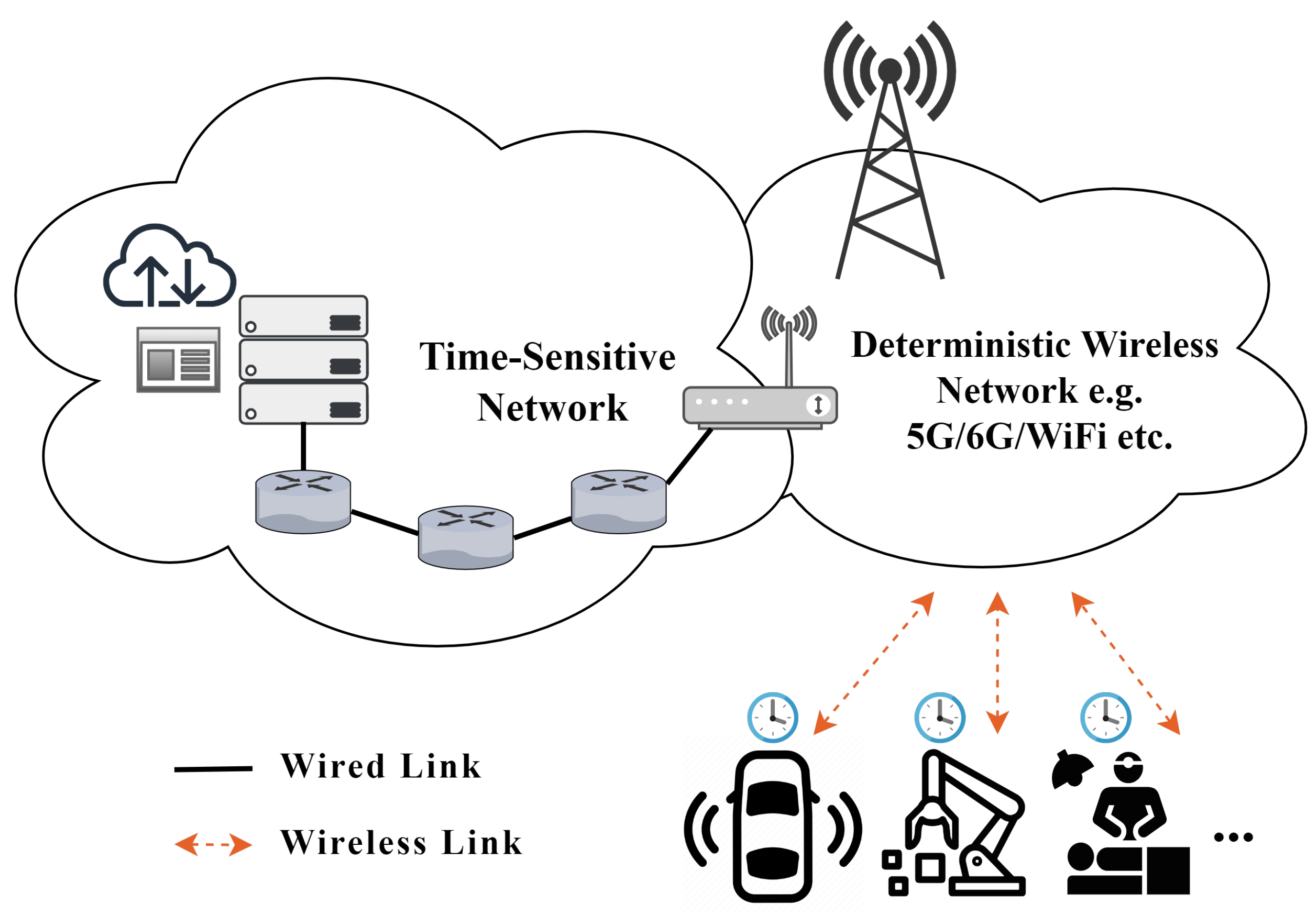
Figure 2.
Diagram of the research problem.

Figure 3.
Diagram of the delay PDF.

Figure 4.
Parameter estimation process.
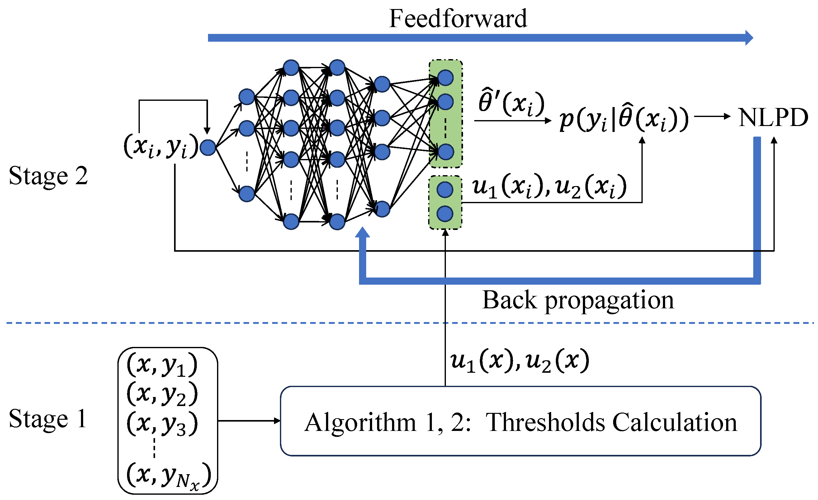
Figure 5.
Graphical characteristics of .
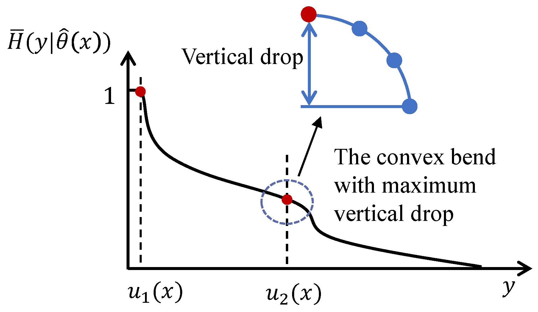
Figure 6.
Mean and fluctuation amplitude of tail probability distributions trained using the SDR WiFi downlink delay dataset sampled at a sampling ratio of 0.8%.
Figure 6.
Mean and fluctuation amplitude of tail probability distributions trained using the SDR WiFi downlink delay dataset sampled at a sampling ratio of 0.8%.
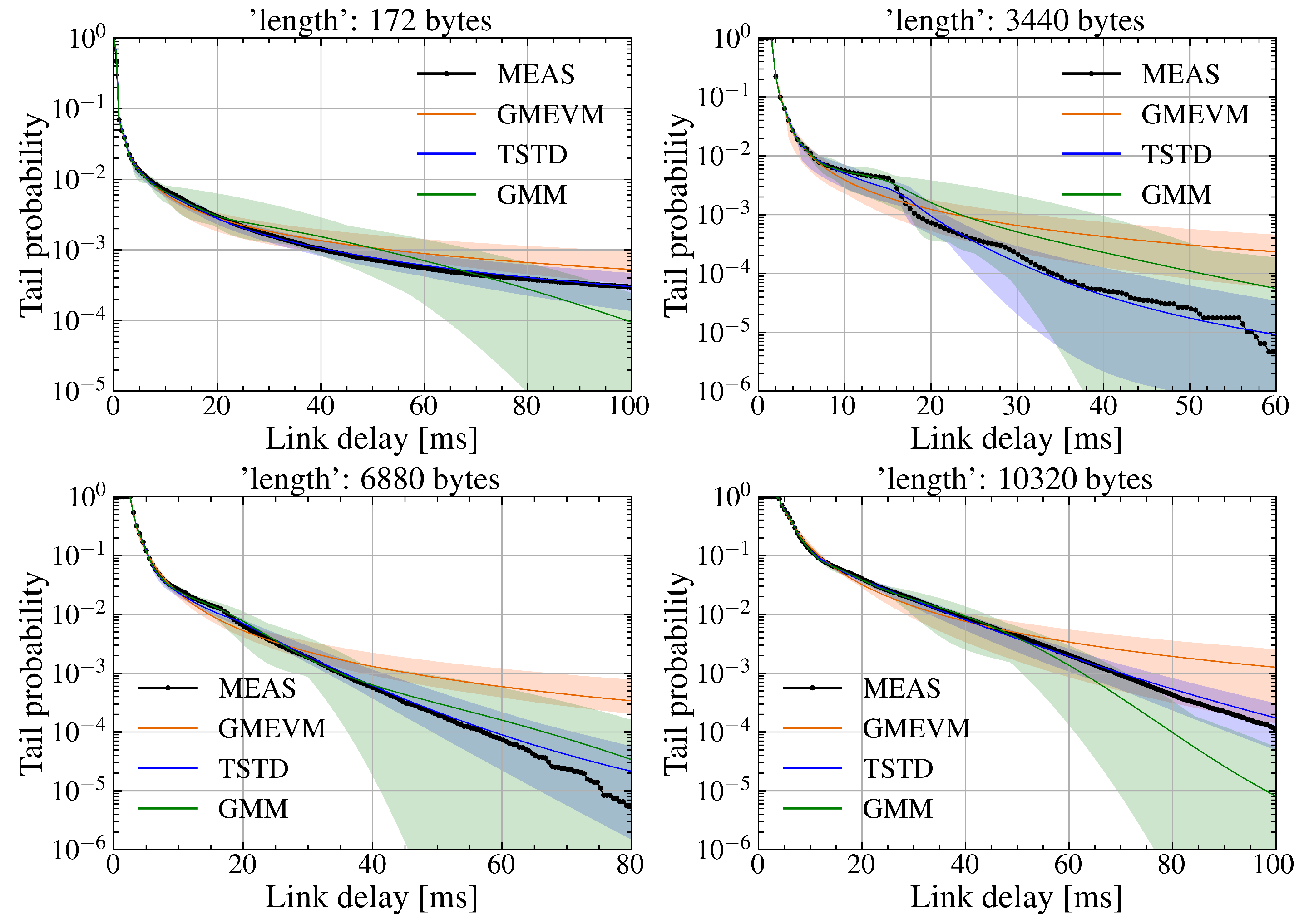
Figure 7.
Mean and fluctuation amplitude of tail probability distributions trained using the SDR WiFi downlink delay dataset sampled at a sampling ratio of 6.25%.
Figure 7.
Mean and fluctuation amplitude of tail probability distributions trained using the SDR WiFi downlink delay dataset sampled at a sampling ratio of 6.25%.
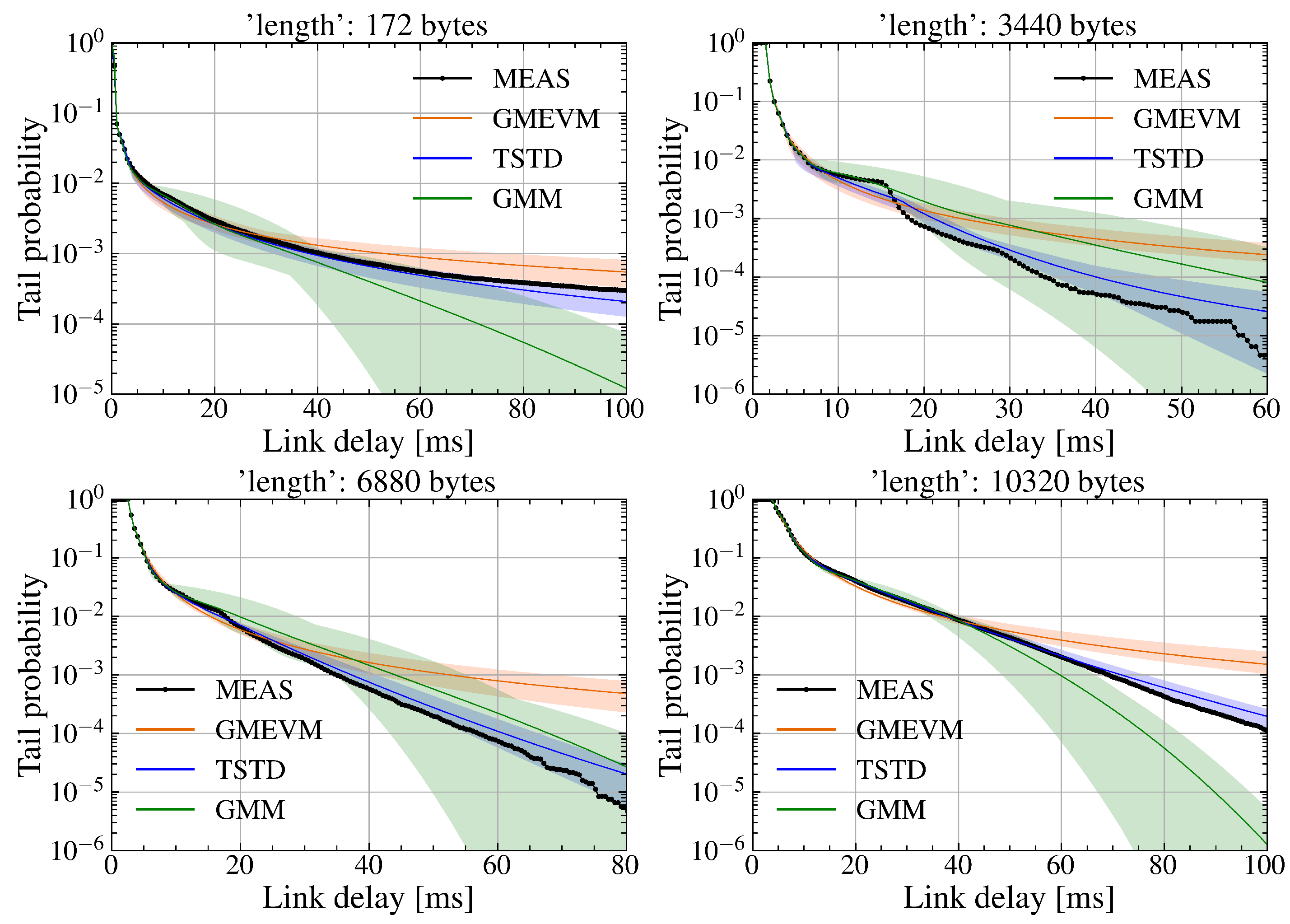
Figure 8.
Mean and fluctuation amplitude of tail probability distributions trained using the SDR WiFi downlink delay dataset sampled at a sampling ratio of 21%.
Figure 8.
Mean and fluctuation amplitude of tail probability distributions trained using the SDR WiFi downlink delay dataset sampled at a sampling ratio of 21%.
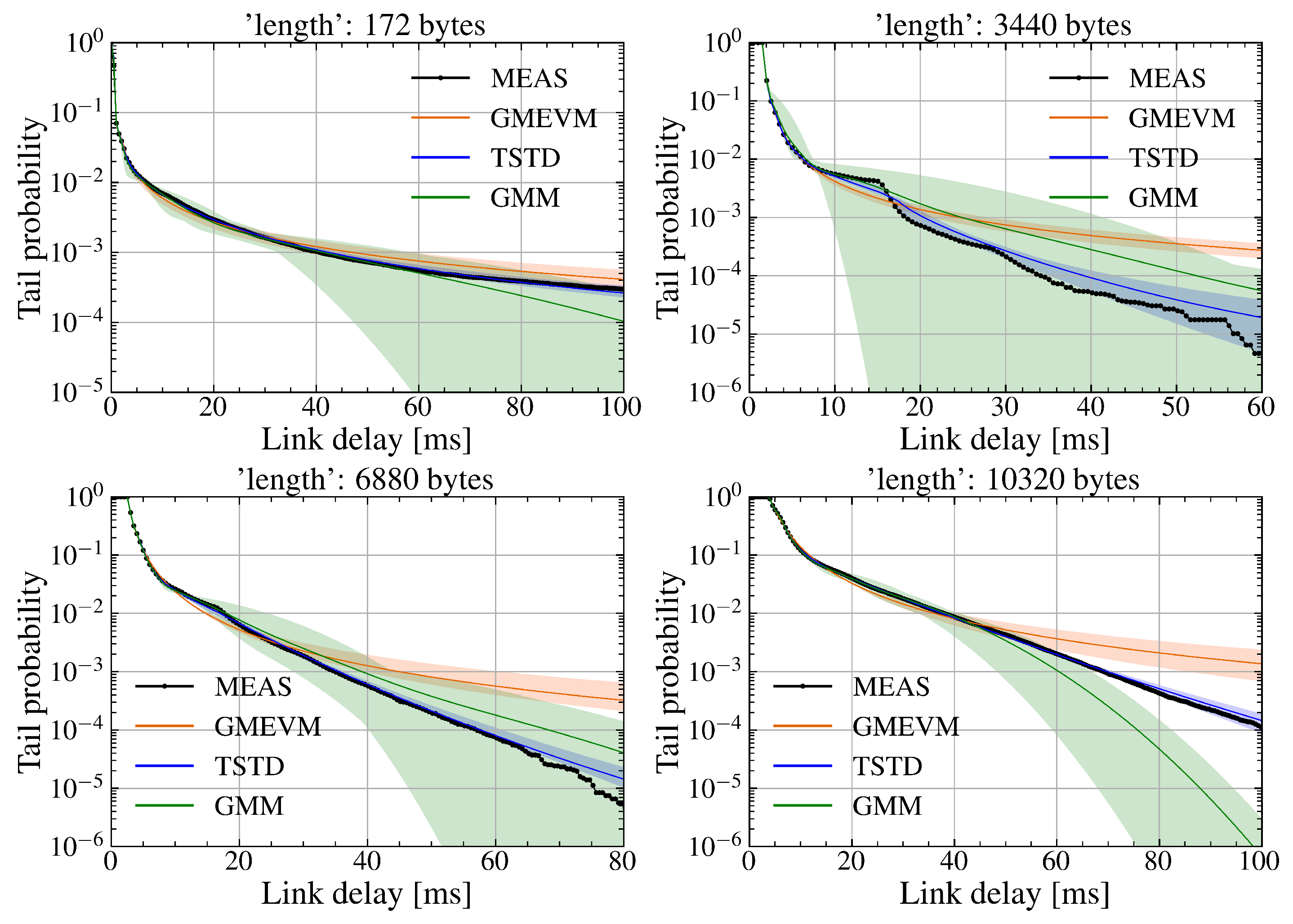
Figure 9.
Mean and fluctuation amplitude of tail probability distributions trained with I = 20 and a sampling ratio of 21% for GMM.
Figure 9.
Mean and fluctuation amplitude of tail probability distributions trained with I = 20 and a sampling ratio of 21% for GMM.
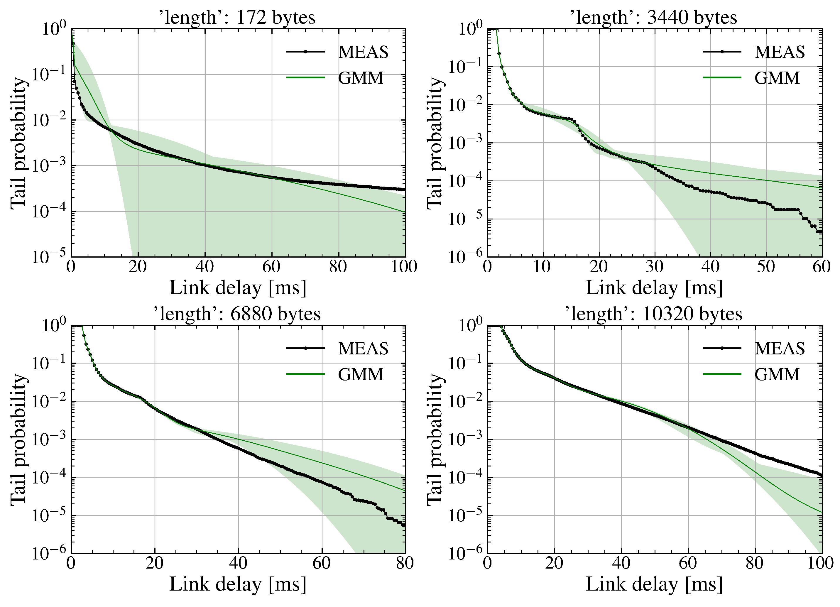
Figure 10.
Mean and fluctuation amplitude of tail probability distributions trained using the SDR WiFi downlink delay dataset sampled at a sampling ratio of 100%.
Figure 10.
Mean and fluctuation amplitude of tail probability distributions trained using the SDR WiFi downlink delay dataset sampled at a sampling ratio of 100%.
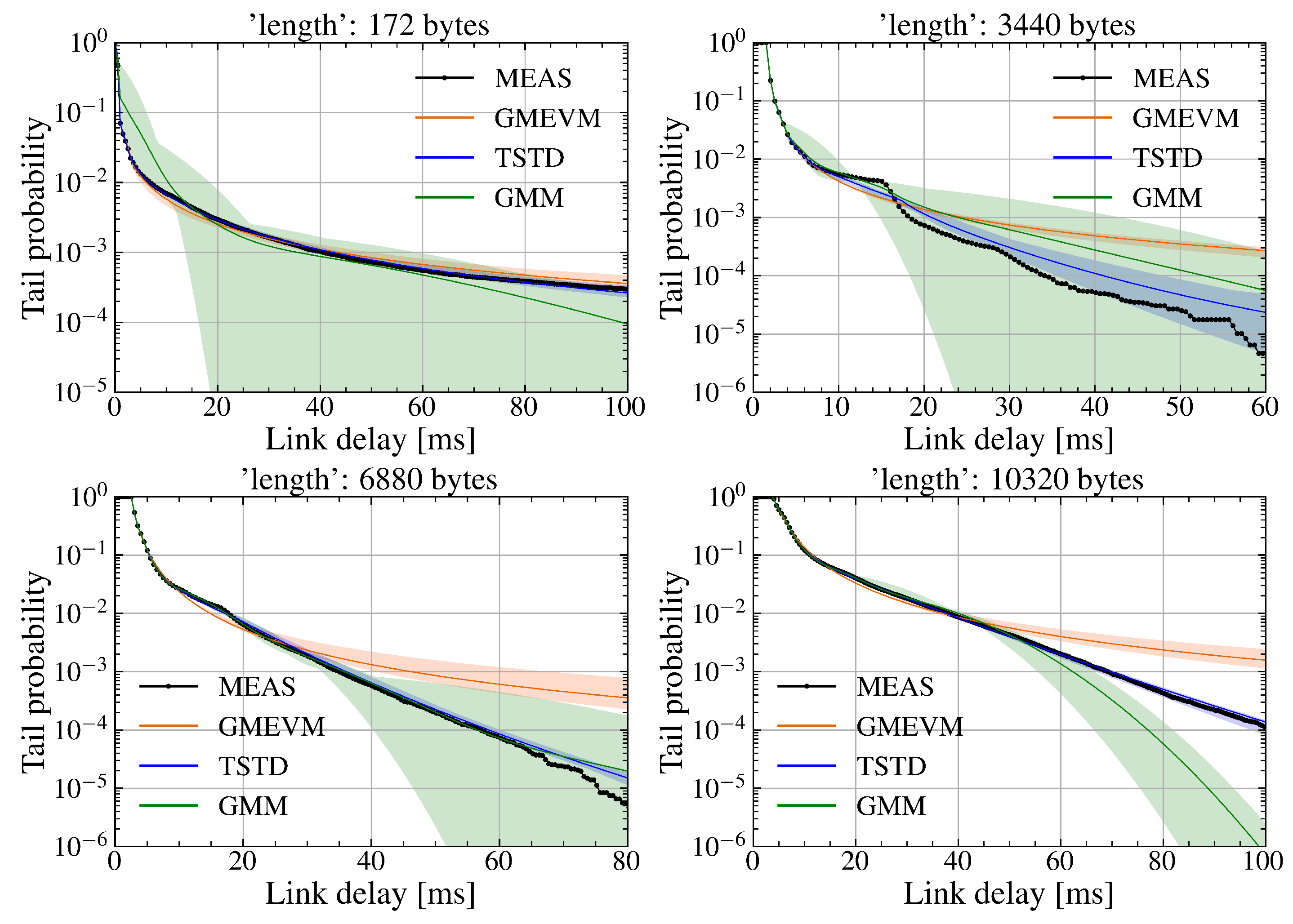
Figure 11.
Mean and fluctuation amplitude of tail probability distributions trained using the SDR WiFi downlink delay dataset, sampled at a sampling ratio of 21% and with Gaussian noise of 1 ms variance introduced.
Figure 11.
Mean and fluctuation amplitude of tail probability distributions trained using the SDR WiFi downlink delay dataset, sampled at a sampling ratio of 21% and with Gaussian noise of 1 ms variance introduced.
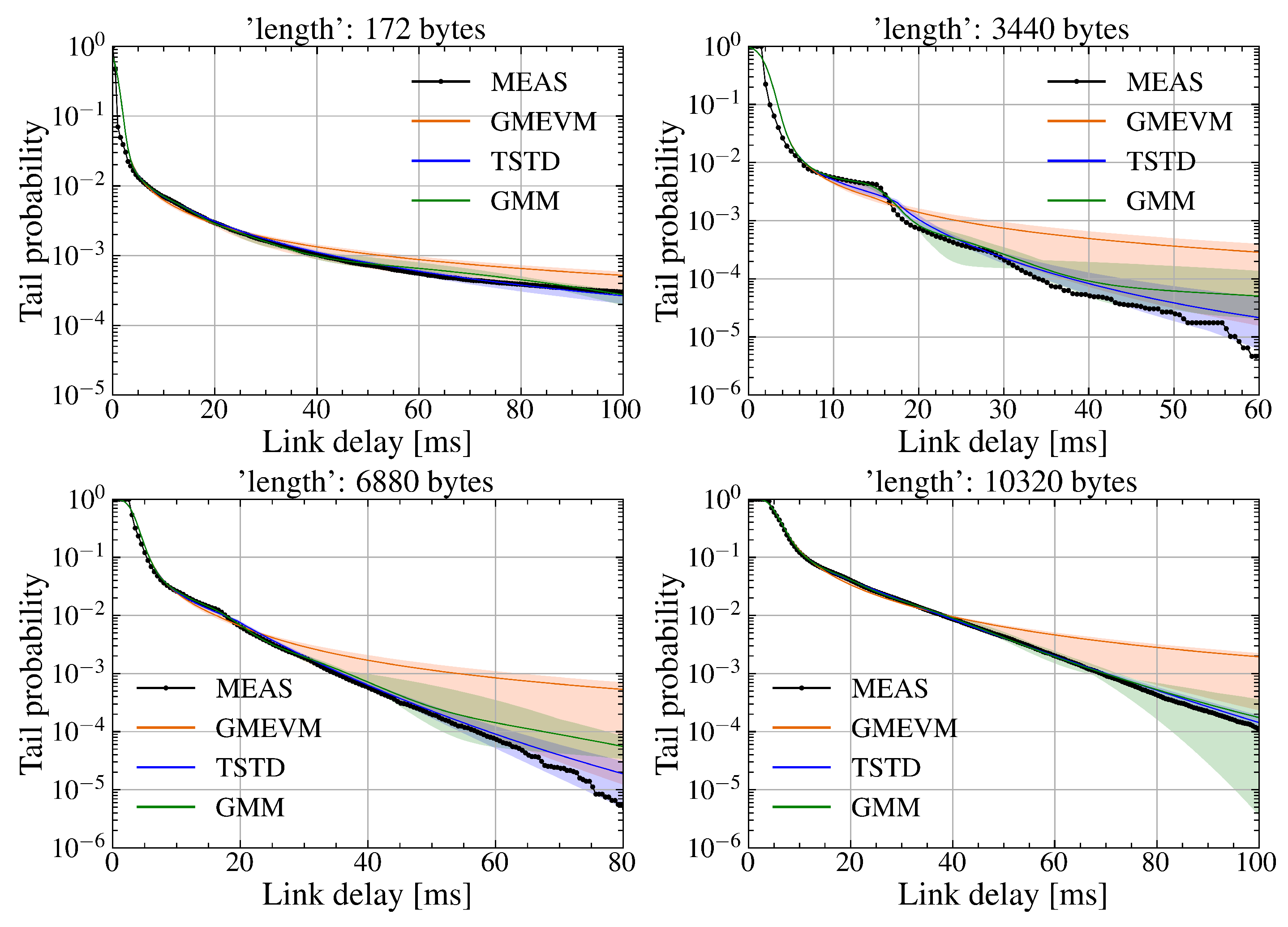
Figure 12.
Mean and fluctuation amplitude of tail probability distributions trained using the SDR WiFi downlink delay dataset, sampled at a sampling ratio of 21% and with Gaussian noise of 3 ms variance introduced.
Figure 12.
Mean and fluctuation amplitude of tail probability distributions trained using the SDR WiFi downlink delay dataset, sampled at a sampling ratio of 21% and with Gaussian noise of 3 ms variance introduced.
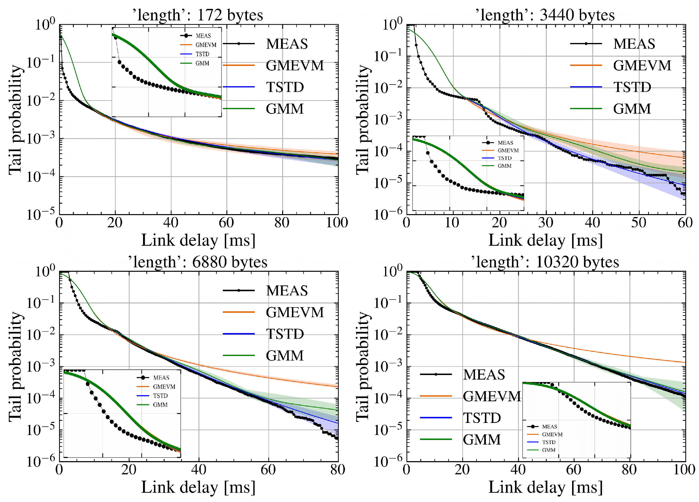

Table 1.
Basic information on SDR WiFi datasets [28].
Table 1.
Basic information on SDR WiFi datasets [28].
| End Node Location | RSSI (dBm) | Downlink Capacity (Mbps) | Packet Length (Bytes) | Number of Samples |
|---|---|---|---|---|
| (1, 0) / (8, 5) | -61 / -87 | 26.22 / 9.26 | 172 | 1256295 |
| (1, 0) | -61 | 26.22 | 3440 | 1075910 |
| (1, 0) | -61 | 26.22 | 6880 | 1068077 |
| (1, 0) | -61 | 26.22 | 10320 | 1036423 |
1 RSSI refers to the received signal strength indication.
Table 2.
Segmentation thresholds for packets of different lengthss.
| Packet Length (Bytes) | ||
|---|---|---|
| 172 | 0.5 | 10.5 |
| 3440 | 2.0 | 14.0 |
| 6880 | 3.0 | 16.0 |
| 10320 | 4.5 | 17.5 |
Table 3.
Average training time under different sampling rates, .
| Sampling Ratio | GMM | GMEVM | TSTD |
|---|---|---|---|
| 26 sec. | 42 sec. | 44.7 sec. | |
| 2.07 min. | 3.93 min. | 4.19 min. | |
| 10.56 min. | 15.15 min. | 15.54 min. |
Table 4.
and of tail probabilities.
| GMM | GMEVM | TSTD | |
|---|---|---|---|
| 172 bytes | |||
| 0.0004848 | 0.0005824 | 0.0004531 | |
| 0.0013418 | 0.0009624 | 0.0006790 | |
| 3440 bytes | |||
| 0.0002742 | 0.0002565 | 0.0000752 | |
| 0.0025520 | 0.0003158 | 0.0002115 | |
| 6880 bytes | |||
| 0.0002252 | 0.0005638 | 0.0001192 | |
| 0.0014704 | 0.0006953 | 0.0005775 | |
| 10320 bytes | |||
| 0.0005072 | 0.0018821 | 0.0001714 | |
| 0.0032255 | 0.0027527 | 0.0003937 | |
Table 5.
MAEs of tail probabilities at some delay values.
| GMM | GMEVM | TSTD | TSTD vs. GMM |
TSTD vs. GMEVM |
|
|---|---|---|---|---|---|
| 172 bytes | |||||
| 10 ms | 0.0001161 | 0.0009614 | 0.0002117 | — | — |
| 20 ms | 0.0003119 | 0.0002654 | 0.0000280 | ↓ | ↓ |
| 40 ms | 0.0002604 | 0.0001805 | 0.0000621 | — | ↓ |
| 60 ms | 0.0000448 | 0.0001994 | 0.0000344 | — | ↓ |
| 80 ms | 0.0001462 | 0.0001483 | 0.0000140 | ↓ | ↓ |
| 3440 bytes | |||||
| 10 ms | 0.0000116 | 0.0012004 | 0.0003190 | ↑ | ↓ |
| 20 ms | 0.0010484 | 0.0006407 | 0.0003960 | ↓ | — |
| 40 ms | 0.0002370 | 0.0004430 | 0.0000422 | ↓ | ↓ |
| 60 ms | 0.0000520 | 0.0002714 | 0.0000150 | — | ↓ |
| 80 ms | 0.0000114 | 0.0001795 | 0.0000035 | ↓ | |
| 6880 bytes | |||||
| 10 ms | 0.0019739 | 0.0015411 | 0.0009512 | ↓ | ↓ |
| 20 ms | 0.0013008 | 0.0013864 | 0.0002981 | ↓ | ↓ |
| 40 ms | 0.0003517 | 0.0006850 | 0.0000295 | ↓ | ↓ |
| 60 ms | 0.0001067 | 0.0004947 | 0.0000053 | ||
| 80 ms | 0.0000360 | 0.0003199 | 0.0000091 | ↓ | |
| 10320 bytes | |||||
| 10 ms | 0.0025418 | 0.0172135 | 0.0009030 | ↓ | |
| 20 ms | 0.0013047 | 0.0076196 | 0.0013923 | — | — |
| 40 ms | 0.0000938 | 0.0006340 | 0.0003321 | ↑ | — |
| 60 ms | 0.0009785 | 0.0016258 | 0.0000657 | ↓ | |
| 80 ms | 0.0003885 | 0.0016749 | 0.0000819 | ↓ | |
2 The values in columns 2-4 denote MAEs. The meanings of the symbols in columns 5 and 6 are as follows. For TSTD, compared with GMM or GMEVM, the symbol ’—’ represents that MAE remains the same in the order of magnitude; and the symbols ’↓’, ’’, and ’↑’ represent that MAE decreases by one order of magnitude, decreases by two orders of magnitude, and increases by one order of magnitude, respectively.
Table 6.
AFAs of tail probabilities at some delay values.
| GMM | GMEVM | TSTD | TSTD vs. GMM |
TSTD vs. GMEVM |
|
|---|---|---|---|---|---|
| 172 bytes | |||||
| 10 ms | 0.0039507 | 0.0019459 | 0.0004887 | ↓ | ↓ |
| 20 ms | 0.0021704 | 0.0009179 | 0.0004761 | ↓ | — |
| 40 ms | 0.0012367 | 0.0005630 | 0.0001728 | ↓ | — |
| 60 ms | 0.0009629 | 0.0004137 | 0.0001308 | — | — |
| 80 ms | 0.0005695 | 0.0003291 | 0.0001165 | — | — |
| 3440 bytes | |||||
| 10 ms | 0.0073440 | 0.0010459 | 0.0008199 | ↓ | ↓ |
| 20 ms | 0.0054414 | 0.0005337 | 0.0006164 | ↓ | — |
| 40 ms | 0.0012082 | 0.0002552 | 0.0000718 | ↓ | ↓ |
| 60 ms | 0.0001327 | 0.0001636 | 0.0000345 | ↓ | ↓ |
| 80 ms | 0.0000365 | 0.0001188 | 0.0000171 | — | ↓ |
| 6880 bytes | |||||
| 10 ms | 0.0044745 | 0.0023440 | 0.0035819 | — | — |
| 20 ms | 0.0101731 | 0.0015240 | 0.0020221 | ↓ | — |
| 40 ms | 0.0017925 | 0.0009852 | 0.0001703 | ↓ | — |
| 60 ms | 0.0005073 | 0.0006320 | 0.0000407 | ↓ | ↓ |
| 80 ms | 0.0001442 | 0.0004451 | 0.0000130 | ↓ | ↓ |
| 10320 bytes | |||||
| 10 ms | 0.0173197 | 0.0219340 | 0.0022661 | ↓ | ↓ |
| 20 ms | 0.0147038 | 0.0021904 | 0.0013999 | ↓ | — |
| 40 ms | 0.0066856 | 0.0039259 | 0.0006537 | ↓ | ↓ |
| 60 ms | 0.0021740 | 0.0029630 | 0.0002614 | ↓ | ↓ |
| 80 ms | 0.0001569 | 0.0022165 | 0.0001964 | — | ↓ |
3 The values in columns 2-4 denote AFAs. The meanings of the symbols in columns 5 and 6 are as follows. For TSTD, compared with GMM or GMEVM, the symbol ’—’ represents that AFA remains the same in the order of magnitude; and the symbol ’↓’ represents that AFA decreases by one order of magnitude.
Disclaimer/Publisher’s Note: The statements, opinions and data contained in all publications are solely those of the individual author(s) and contributor(s) and not of MDPI and/or the editor(s). MDPI and/or the editor(s) disclaim responsibility for any injury to people or property resulting from any ideas, methods, instructions or products referred to in the content. |
© 2025 by the authors. Licensee MDPI, Basel, Switzerland. This article is an open access article distributed under the terms and conditions of the Creative Commons Attribution (CC BY) license (http://creativecommons.org/licenses/by/4.0/).
Copyright: This open access article is published under a Creative Commons CC BY 4.0 license, which permit the free download, distribution, and reuse, provided that the author and preprint are cited in any reuse.


