Submitted:
19 May 2025
Posted:
19 May 2025
You are already at the latest version
Abstract
Accurate detection of anomalous ship behavior in AIS data remains challenged by signal noise and dynamic maritime patterns. While the Space-air-ground-sea integrated network (SAGSIN) technology has significantly reduced transmission delays and interruptions in maritime AIS communications that previously relied on remote satellite connections, anomalies still occur due to sensor errors and other factors. Identifying these anomalies is critical for maritime safety, efficient transportation management, and security surveillance, but faces challenges in signal quality, pattern complexity, and real-time processing requirements. We propose EASY, a novel framework integrating exponential attention with state-space models for fine-grained anomaly detection. By reformulating the task as token classification, EASY enables precise identification of abnormal trajectory segments while modeling multi-scale temporal dependencies. Evaluations on real-world port data demonstrate SOTA performance of 76.10% in F1, surpassing other models by 11.32%.
Keywords:
Exponential Attention
; State-space Models
; AIS Anomaly Detection
; Maritime Safety
1. Introduction
With the evolution of the Space-air-ground-sea integrated network (SAGSIN), maritime communications have undergone significant improvements, enhancing the reliability and coverage of ship monitoring systems. The Automatic Identification System (AIS), which transmits navigation data through integrated maritime transceivers, satellite relays, and ground stations, benefits greatly from these advancements. Previously, poor network conditions often resulted in AIS transmission delays and signal anomalies, limiting the practical application of AIS-based behavior analysis. However, with SAGSIN enhancements, communication quality has substantially improved, reducing delays, data loss, and signal anomalies. This increased reliability elevates the effectiveness of AIS-based anomaly detection systems, supporting maritime safety monitoring and ship-shore integrated management through communication networks.
Despite these improvements, sensor errors remain a critical challenge in maritime anomaly detection. The significance of this challenge has grown as maritime safety and security demands increase. Our research focuses on developing robust anomaly recognition models that can distinguish between genuine behavioral anomalies and sensor-induced errors. These models maintain high performance even when processing imperfect sensor data, enabling accurate prediction and enhanced safety management. This capability is particularly important as maritime transportation systems become increasingly automated and dependent on reliable anomaly detection mechanisms.
Abnormal behavior is defined as a characteristic that is significantly different from normal navigation behavior. Existing studies have used ship kinematic characteristics[1,2] and radar signal[3] to judge the state of a ship. As one of the most important data sources for ships, AIS has become the core data support for studying ship behavior. Abnormal behavior detection methods based on AIS data[3] include but are not limited to the following categories: 1) Methods based on detection models, which usually automatically learn normal behavior patterns through machine learning or deep learning models, and identify behaviors that deviate from the pattern; 2) rule-based detection methods, which use expert experience or existing knowledge to build a rule base to judge ship behavior; 3) Statistical methods, which identify low-probability or rare events by modeling historical behavior data; fourth, methods based on Markov chains, which establish state transition models to characterize the dynamic evolution of ship behavior, thereby identifying behaviors that do not conform to the transition rules; 4) Some other methods, such as emerging technologies based on cluster analysis, graph neural networks, spatiotemporal graph modeling, etc., which are gradually introduced into the research of anomaly detection.
Behavioral anomalies[4] in AIS tracks often indicate unsafe or non-compliant navigational behavior, including U-turns, circular drifts, unexplained detours, and noise-like position shifts. These patterns may reflect potential risks[5], such as navigational oversights, equipment failures, or intentional manipulation of AIS signals. If undetected, such anomalies may result in serious maritime incidents, including ship collisions, traffic jams, unauthorized entry into restricted areas, and even property and human casualties. Therefore, the ability to detect these behaviors in a timely and accurate manner is critical to ensuring maritime safety and operational integrity.
In recent studies, different scholars have sought the characteristics of abnormal ship behavior from a potential perspective[6,7,8]. To overcome these challenges, we propose EASY (Exponential Attention for State-Space Yearning Networks), a novel deep learning framework tailored for fine-grained ship behavior anomaly detection. Unlike previous approaches that may struggle with sensor-induced errors, EASY is designed to operate effectively within the improved SAGSIN environment where communication reliability has increased but sensor-level anomalies still persist. The framework leverages state-space representation to capture ship dynamics and embeds an exponential attention mechanism to model long-range dependencies in AIS sequences—enhancing the detection of both local and global behavior changes. This approach takes advantage of the reduced transmission delays and interruptions provided by SAGSIN while addressing the remaining sensor-level error challenges. Importantly, we formulate the detection task as a token classification problem, enabling our model to assign behavior labels at each time step, distinguishing between normal motion and various categories of abnormal behaviors: U-turns, cyclic patterns, noisy drifts, and detour paths. This granular detection capability is particularly valuable in the context of improved but still imperfect sensor data transmission within maritime environments.
Experimental results on a real AIS dataset demonstrate that EASY achieves state-of-the-art performance in both accuracy and interpretability, outperforming existing models in identifying complex behavior anomalies under realistic noisy conditions. These findings highlight the potential of integrating advanced sequence modeling techniques in the SAGSIN environment to enhance maritime situational awareness and proactively mitigate security risks.
The main contributions of this study to AIS-based vessel behavior anomaly detection are as follows:
- A fine-grained, token-level annotation scheme is proposed, defining five behavioral categories—Normal, U-Shape Turn, Cycle, Noise, and Detour, which are all based on real-world AIS trajectories. This dataset serves as a public benchmark for evaluating and comparing anomaly detection methods in maritime domains.
- This is the first work to formulate AIS trajectory anomaly detection as a token classification task, enabling sequential modeling at a fine temporal resolution and offering more precise identification of anomalous segments within vessel tracks.
- A novel hybrid architecture is proposed to integrate an exponential moving attention mechanism with a state-space-based Yearning network. Leveraging the low-latency benefits provided by SAGSIN, the proposed model demonstrates enhanced effectiveness in detecting abnormal ship characteristics.
2. Related Work
Statistical modeling has been widely applied in the domain of vessel behavior anomaly detection. Gaussian Mixture Models (GMM) [9] are frequently employed to model the distribution of vessel behavior data by combining multiple Gaussian components to capture complex dynamics. For instance, Chen et al. proposed a GMM-based anomaly detection method where vessel movement patterns are assumed to originate from multiple latent distributions, enabling effective identification of abnormal behavior [10]. Similarly, Xie et al. [11] developed a trajectory anomaly detection approach that classifies trajectory points using changes in direction and speed, achieving robust detection of U-turns, loops, and other abnormal patterns.
Kernel Density Estimation (KDE), a non-parametric technique, has also been utilized to estimate the probability density function of trajectory data for anomaly detection. Dai et al. [12] adopted KDE to model AIS trajectory distributions and identify outliers based on low-probability regions. Hidden Markov Models (HMMs) [13] have been used to model temporal dependencies within trajectory sequences by learning state transitions and observation likelihoods. In addition, Conditional Random Fields (CRFs) [14] have been leveraged for sequence labeling tasks, capturing contextual dependencies in vessel behavior. Grid-based methods, on the other hand, divide trajectory space into discrete regions to discover behavioral patterns and identify potential anomalies efficiently. Moreover, the Ornstein–Uhlenbeck process has been adopted for modeling vessel behavior dynamics. Zaman et al. [15] proposed an online anomaly detection and behavior classification framework based on this process, capable of tracking deviations in AIS streams in real-time.
Statistics-based machine learning approaches have demonstrated substantial progress in this field. Clustering methods, especially density-based techniques such as DBSCAN [16] and its variants, are widely used to identify abnormal behavior without supervision. DBSCAN detects anomalies by identifying low-density regions and has been successfully applied to vessel trajectory data. HDBSCAN [17], a hierarchical variant of DBSCAN, improves clustering robustness through adaptive density estimation, making it suitable for capturing complex maritime behaviors. Through unsupervised clustering, these methods can automatically reveal underlying behavior patterns and detect outliers with minimal human intervention. Jiao and Li [18] proposed a KD-Tree optimized DBSCAN algorithm, significantly accelerating the detection process while enhancing accuracy. In addition, trajectory-based clustering approaches further integrate AIS features and construct multi-scale cluster structures for detecting route-specific anomalies [19]. Yan et al. [20] combined spatial and semantic information of AIS trajectories using graph-based clustering algorithms, achieving reliable detection across multiple coastal regions in China. While such methods are well-suited for large-scale offline analysis with limited labeling requirements, they often struggle with rare or previously unseen anomalous patterns.
Deep learning techniques have become increasingly prevalent in vessel anomaly detection tasks. Convolutional Neural Networks (CNNs) [21] are capable of learning spatial and dynamic patterns from trajectory representations, offering powerful feature extraction capabilities. Deep Neural Networks (DNNs), as general-purpose nonlinear models, can effectively learn complex behavior patterns from sequential data, particularly in large-scale settings. Recurrent neural networks (RNNs), especially Long Short-Term Memory (LSTM) [22] and Gated Recurrent Unit (GRU) [23] models, have proven effective in capturing temporal dependencies within maritime behaviors. LSTM is particularly adept at learning long-term dependencies, while GRU offers a simplified alternative with improved training efficiency, making it well-suited for real-time detection tasks.
Hybrid approaches combining Deep RNNs with trajectory clustering have been shown to enhance detection granularity by modeling multi-modal trajectory features such as speed, course, and position [24]. The heatmap Laplacian diffusion framework integrates graph structures with sequential modeling to enhance spatiotemporal anomaly detection performance in AIS data [25]. Furthermore, the Gaussian Mixture Variational Autoencoder (GMVAE)-based framework detects anomalies by analyzing reconstruction errors and posterior cluster probabilities, showing increased robustness in weakly supervised settings [26]. Nevertheless, deep learning methods face challenges in generalization and interpretability, especially in novel environments, edge cases, or data-scarce scenarios. High training costs and substantial computational requirements also remain significant barriers to large-scale deployment.
In summary, although statistical modeling, machine learning, and deep learning approaches have each achieved varying degrees of success in maritime anomaly detection, they also exhibit inherent limitations. Statistical methods often rely on strong assumptions and are inadequate for capturing nonlinear or high-dimensional patterns. Machine learning models provide flexibility but can be data-hungry and computationally expensive. Deep learning techniques offer superior performance but are susceptible to overfitting and may lack generalizability in complex or evolving maritime environments. Therefore, a key research challenge lies in how to effectively integrate the strengths of these approaches while mitigating their respective drawbacks. Chapter Section 3 presents our proposed hybrid framework that addresses these limitations by combining model interpretability, scalability, and adaptability for practical maritime anomaly detection.
3. Methodology
This section introduces the dataset processing method and the architecture of the proposed EASY model. This study utilizes AIS data collected from ships in the Ningbo-Zhoushan port area. The dataset is collected from hifleet by scrapy. The data contains navigation information of about 500 ships with valid AIS transmissions. The diverse ship traffic in this area provides an ideal cases for evaluating our proposed EASY architecture.
3.1. Abnormal Definition
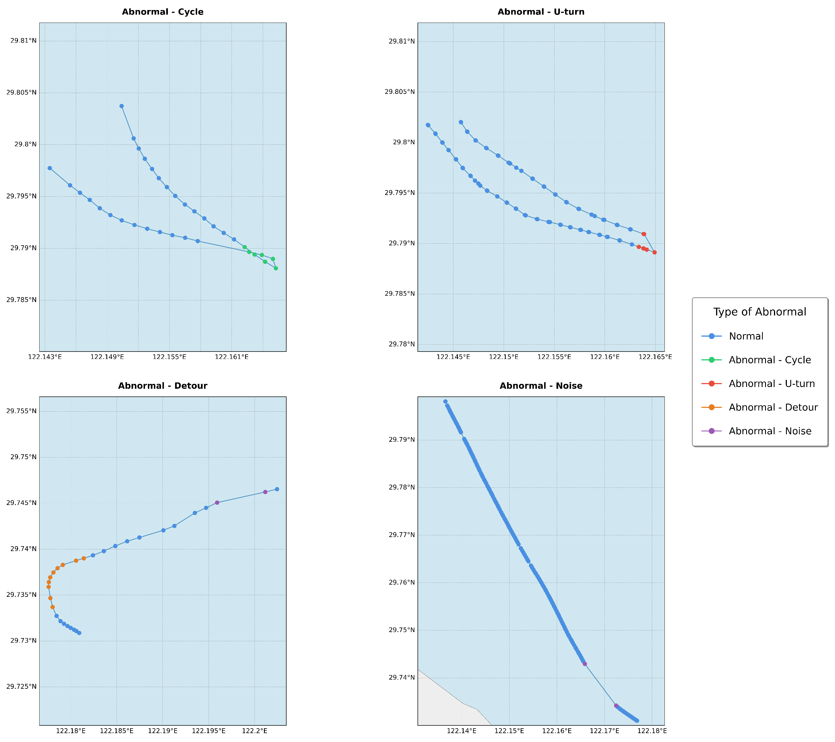
Following the annotation methodology proposed by Rong et al.[4], we developed a comprehensive labeling scheme tailored to our specific dataset. This scheme categorizes trajectory behaviors into five distinct types: one representing normal movement and four representing abnormal patterns. The abnormal trajectory types include Cycle, U-turn, Detour, and Noise, each reflecting a particular deviation from expected or efficient movement behavior.
- 0 - Normal: Smooth, goal-directed trajectories that follow an expected and efficient path.
- 1 - Cycle: Repetitive a loop within a confined area.
- 2 - U-turn: Abrupt reversals in direction, over to 180 degrees.
- 3 - Detour: Significant deviations from the shortest or expected path, usually due to obstructions or errors.
- 4 - Noise: Irregular, fragmented movements lacking continuity, typically caused by sensor errors or random disturbances.
This annotation framework allows for a nuanced interpretation of movement behavior, enabling downstream tasks such as anomaly detection, trajectory prediction, and behavior modeling to be grounded in semantically rich, high-resolution labels. Figure 1 gives examples to distinguish different types of anomalies. By distinguishing between specific abnormal patterns, our approach enhances both the interpretability and diagnostic power of trajectory analysis models.
Figure 1.
Four different types of abnormal behavior.
3.2. Data Processing
The data processing flow involves two primary steps: data cleaning and feature extraction. In data cleaning, erroneous, missing, or incomplete entries are removed from raw AIS data to maintain consistency and integrity. Cubic spline interpolation is applied to address potential gaps in time series data, enhancing data quality. A sliding window technique facilitates improved comparison between actual and predicted values within local windows. Feature extraction includes computing kinematic variables such as acceleration and angular velocity, alongside the introduction of the detour and yaw angle factors, which are crucial for analyzing ship behavior and detecting anomalies.
3.2.1. Data Cleaning
Raw AIS data exhibit several notable characteristics: large volume, wide range of features, sparse valid data, information drift, and data gaps. While abnormal detection of ship behaviors still remain a challenge, the implementation of Space-Air-Ground-Sea Integrated Network (SAGSIN) significantly enhances AIS data quality through its multi-terminal communication advantages, providing lower latency and reduced data loss rates. These improvements in AIS transmission reliability make the study of vessel anomaly detection more feasible. For this study, we focus on AIS records from the Port of Ningbo-Zhoushan as the research object, leveraging the enhanced data quality made possible by SAGSIN methods. The data cleaning process consists of several key steps:
Filtering
The first step involves selecting the Area of Interest (AOI) from the vast AIS dataset, which requires filtering based on the geographical coordinates (latitude and longitude) of the vessels. Subsequently, vessels in a moored or anchored state are excluded. These vessels are identified by characteristics such as a travel distance of less than or equal to 5 nautical miles or a constant speed of 0 knots. Next, we select vessels with continuous and complete data points. This rule primarily addresses the temporal aspect of the data, stipulating that the time interval between consecutive data points for a given vessel must not exceed 10 minutes. Although related studiesLiu et al. [2] apply a time interval of up to 6 hours, our model’s strict requirement for sequential data points necessitates a more stringent 10-minute threshold. Finally, we impose a limit on the number of data points for each vessel. Specifically, we require that the number of data points for a given vessel is no fewer than 20 and no more than 200.
The process of data extraction, based on the aforementioned criteria, can be summarized as follows:
- Area of Interest: Filter the AIS data based on the vessel’s geographic coordinates (latitude and longitude) to focus on the area of interest.
- Exclusion of moored/anchored vessels: Exclude vessels that are stationary, identified by characteristics such as a travel distance less than 5 nautical miles or a constant speed of 0 knots.
- Temporal Consistency: Select vessels with continuous and complete data points. Ensure that the time interval between consecutive data points is no more than 10 minutes to maintain temporal sequence.
- Data Point Length: Ensure that each vessel has at least 20 data points and no more than 200 data points to avoid data sparsity or excessive data.
Cubic Spline Interpolation
Currently, many interpolation methods[27,28,29] are used to compensate for the discontinuities of ship values. Cubic spline interpolation[2,27] is employed to address missing or incomplete data in AIS time series. There are often gaps in the time series due to missing or incomplete records, especially in AIS data. Cubic spline interpolation can effectively address this issue by estimating the missing values while preserving the temporal consistency of the data. This technique ensures that the resulting data is both smooth and accurately reflects the underlying trends.
The recorded time in AIS is converted to a timestamp in seconds, with each timestamp adjusted by subtracting the minimum time value as a padding technique. This allows us to treat time as the independent variable x, and use the longitude, latitude, speed, and course over ground (COG) as the dependent variables y for interpolation.
The general form of a cubic spline interpolation for a given interval is given by the following in eq:cubicspline.
where , , , and are the coefficients determined based on the boundary conditions and the data points. These coefficients are computed by solving a system of linear equations that ensures the continuity and smoothness of the spline at the data points.
The cubic spline interpolation method guarantees that the first and second derivatives of the spline are continuous across the entire data set, providing a smooth and natural fit to the data. The resulting interpolation can be used to estimate the missing values in the AIS data, thus enhancing the quality of the dataset and improving the accuracy of the model.
Given the periodic nature of vessel trajectories, directly utilizing global data for validation may not effectively capture the underlying trends or periodicities. To address this limitation, the interpolation process incorporates a sliding window approach of length 10, which is applied to evaluate the predicted values against the real values within each local window. This method is particularly advantageous when the data exhibits varying trends or periodic behavior that cannot be adequately captured by a global cubic spline fit.
In order to perform interpolation, the average distance between adjacent points in the track is first calculated. If the distance between any two adjacent points is greater than , the number of interpolation points t is defined in eq:meant.
Where is the actual distance between two adjacent points i and j, and is rounded up. In other words, if the distance between two adjacent points exceeds the average distance , t timestamp points need to be inserted between the two points to ensure the integrity of the trajectory. The interpolated points will be evenly distributed according to the timestamps and corresponding longitudes and latitudes to supplement the missing trajectory data.
The cubic spline accurately interpolates the original data points, as demonstrated by its interpolation property, which is illustrated in Figure 4. Additionally, the plot presents a smooth, continuous curve that bridges the gaps between sampled points, effectively handling the presence of missing data.
As shown in Figure 5, the error associated with the point interval reconstructed using the cubic method is minimal. Notably, during the data preprocessing phase, we restricted the use of data to intervals of 10 minutes. This constraint significantly contributes to the accuracy of the results.
3.2.2. Feature Extraction
To create an appropriate classification model that captures the observed abnormal behavior of the ship, several features can be derived from the initial data, which includes time, longitude, latitude, heading angle, SOG (Speed Over Ground), and bow angle. Besides, two factor are introduced to help futher understanding the abnormal behaviors of vessel. These features can help distinguish between normal and abnormal vessel behavior and provide meaningful inputs to the model.
Kinematic Variables
Based on AIS data and fundamental kinematic principles [2], we compute acceleration and angular velocity, denoted as and , respectively. The acceleration represents the rate of change of the vessel’s speed, while the angular velocity measures the rate of change of its heading angle. These kinematic variables are essential for analyzing the vessel’s movement dynamics and can provide insights into its navigational behavior and performance.
Detour Factor
In the field of transportation, detour factor (DF) [30] is a commonly used indicator to measure the degree of detour of a path. eq:detourfactor defines the detour factor, which expresses the ratio of the sum of the distances between points on a path to the straight-line distance from the start point to the end point.
The detour factor quantifies the degree of detour of a path by calculating the Euclidean distance between two adjacent points on the path, summing up these distances, and comparing them with the straight-line distance between the start point and the end point. By calculating the detour factor, the severity of abnormal paths can be evaluated and strong data support can be provided for the optimization of transportation.
Yaw Angle Factor
Inspired by the detour factor in eq:detourfactor, we introduce the setting of the yaw factor in eq:avgyawanglefactor. In maritime navigation, the average yaw angle factor (YAF) can be used to assess the overall stability of a vessel’s heading along its entire journey. This factor is computed by averaging the ratio of the absolute difference between the heading angle of the first point and the heading angle of each subsequent point to the initial heading angle.
Where represents the heading angle of the first point, is the heading angle of each point along the path, and n is the total number of points. The average yaw angle factor provides an overall measure of the consistency of the vessel’s heading throughout the journey. A value closer to 1 indicates that the vessel has maintained a stable heading, while a value significantly less than 1 suggests that the vessel has undergone considerable heading changes during its path. This averaged metric is useful for understanding the vessel’s navigational behavior over the entire route and can aid in the optimization of the vessel’s movement strategy.
3.3. Exponential Attention
As illustrated in the Figure 6, an EMA (Exponential Moving Attention) module was incorporated prior to the attention mechanism.The MA (Moving Average) methodology has found extensive applications in sequence analysis tasks, particularly in stock market analysis and anomaly detection. It is primarily proposed to mitigate the influence of local anomalies on overall data patterns. Generally, there are four fundamental implementations of MA: SMA (Simple Moving Average) in eq:ssma, WMA (Weighted Moving Average) in eq:wma, CMA (Cumulative Moving Average) in eq:cma, and EMA (Exponential Moving Average) in eq:ema.
When , SMA can be illustrated in Figure 7.
When , WMA can be illustrated in Figure 8.
When , CMA can be illustrated in Figure 9.
When , EMA can be illustrated in Figure 10.
In the EMA module, the parameter serves as a decay factor controlling the weight distribution of historical data. When takes a larger value, the model assigns higher weight coefficients to current timestep data while reducing dependency on historical data. This mechanism enables EMA to effectively suppress the interference of random fluctuations on overall trends in the sequence. Specifically, as timesteps progress, the weight decay term exhibits exponential decay and converges to zero, thereby achieving adaptive weight attenuation for early data.
The EMA demonstrates superior responsiveness to contemporary network state data, complementing the capabilities of SAGSIN technology. SAGSIN’s primary advantage is providing reliable, low-latency maritime communications, which creates new feasibility for vessel anomaly detection through AIS data analysis. This low-latency characteristic makes it practical to detect critical vessel state transitions and behavioral anomalies in real-time, especially in scenarios demanding immediate responses. While traditional maritime communication systems struggled with data gaps and transmission delays, SAGSIN overcomes these limitations, enabling more comprehensive vessel monitoring. The EMA approach further enhances this capability by facilitating rapid adaptation to dynamic situational changes while minimizing processing delays. Furthermore, EMA’s exponential decay mechanism effectively attenuates the influence of historical AIS data while simultaneously smoothing data irregularities without compromising essential movement pattern information, thereby maintaining robust anomaly detection performance even in complex maritime environments where vessel behaviors constantly evolve.
From a theoretical perspective, the EMA and Convolutional Neural Network (CNN) architectures exhibit fundamental structural analogies, both manifesting as sophisticated adaptive weight modulation mechanisms. The attention mechanism of EMA employs single-head attention to capture complex dependencies within SAGSIN network states. As illustrated in Figure 11, the shift window single-head attention mechanism processes network topology information through a sliding window approach. This mechanism is particularly effective in modeling dynamic relationships between space-air-ground-sea nodes.
The main query of single-head attention is in eq:singleheadattention.
Where , , and represent queries, keys, and values derived from network state matrices, is a dynamic scaling factor adapting to network conditions, and encodes relative positional information of network nodes. This formulation enables the model to effectively capture both local and global dependencies in the heterogeneous SAGSIN architecture, particularly crucial for maintaining connectivity awareness across different network layers.
Within the CNN framework, convolutional kernels facilitate local feature extraction through systematic sliding window operations; conversely, in the EMA paradigm, the weight coefficient functions as a dynamic convolution operator, implementing temporally-dependent progressive weight decay, thereby establishing differentiated weight distributions across temporal input sequences. This adaptive weight modulation methodology substantially enhances the model’s temporal sensitivity to recent data fluctuations while simultaneously achieving optimal attenuation of historical information.
The underlying mechanism demonstrates intrinsic correspondence with the weight-sharing principles and local receptive field characteristics inherent in convolutional operations, conferring upon EMA exceptional sensitivity to temporal trend variations. Through this sophisticated mechanism, EMA effectively attenuates high-frequency perturbations while preserving low-frequency trend information, thus achieving superior signal smoothing and noise suppression capabilities in temporal sequence analysis and predictive modeling applications.
3.4. State space Model
The Structured State Space Models (S4) and Mamba, as typical implementations of State Space Models (SSM) shown in Figure 12, offer critical advantages for vessel trajectory anomaly detection within the SAGSIN framework. Previously, effective vessel anomaly detection was hindered by significant AIS data challenges including signal delays, data loss, and sensor anomalies. SAGSIN’s low-latency communication and rapid switching capabilities between different satellite systems for near and offshore areas have now made AIS-based anomaly detection feasible. Within this improved communication environment, SSMs provide unique capabilities for modeling the sequential nature of vessel trajectory data.
These models map a one-dimensional input function or sequence to an output through a hidden state . The evolution parameter and projection parameters , enable SSMs to capture complex temporal dependencies in vessel movement patterns. This mathematical structure is particularly advantageous for anomaly detection as it can: (1) effectively model normal vessel behavior patterns over extended time sequences, (2) maintain sensitivity to subtle deviations indicating potential anomalies, and (3) adapt to varying noise characteristics in AIS signals that persist even with SAGSIN’s improved transmission reliability. The state-based architecture allows for continuous refinement of vessel behavior understanding, making it superior to traditional methods that struggle with the temporal complexity and irregular sampling of maritime movement data.
In the SAGSIN system, to achieve precise modeling of sea-air-ground transmission signals, S4 and Mamba employ adaptive time discretization methods, introducing dynamic discretization parameter . This parameter automatically adjusts according to multi-level signal transmission characteristics including marine environment, atmospheric transmission, and ground reception, converting continuous system parameters A and B into their discrete forms and . This transformation adopts an optimized zero-order hold (ZOH) method, mathematically expressed as:
Through this discretization process, the system better adapts to multipath effects in marine environments, atmospheric transmission losses, and ground reception interference. The eq:ssm can be reconstructed as:
Specifically, in vessel anomaly state classification tasks, the model implements feature extraction through a global convolution operator, with its adaptive kernel matrix defined as:
The final state recognition output is calculated through:
where represents the structured convolution kernel, and L denotes the length of input sequence x. This design enables the system to effectively process multi-scale temporal features in sea-air-ground signal transmission, providing a reliable mathematical foundation for vessel anomaly detection. Through the Gating mechanism, the model can adaptively adjust feature weights, significantly enhancing signal processing capabilities and classification accuracy in complex marine electromagnetic environments. This method is particularly suitable for handling complex scenarios such as signal attenuation in marine environments, random atmospheric disturbances, and multi-source interference during ground reception, providing robust support for the stable operation of the SAGSIN system.
3.5. Conditional Random Fields
CRF was introduced to strengthen the shortcomings of HMM in feature selection and dependency assumptions. HMM is a generative model that models the joint probability , that is, the joint distribution of the observed data and the label sequence, expressed as the eq:hmm. This requires HMM to make strong assumptions about the relationship between the observed data and the hidden state (such as the independent and identically distributed assumption and the Markov assumption). In contrast, CRF is a discriminative model that directly models the conditional probability without making independence assumptions on the observed data. Therefore, CRF introduces feature functions and weights into the model and maximizes the conditional probability of given observed data by learning these parameters. It is able to directly model the label sequence without assuming the Markov property between the observed data and the hidden state. This enables CRF to better capture long-distance dependencies in the sequence and automatically learn the relationship between features without manually designing features.
The calculation process of CRF involves constructing and optimizing the conditional probability , that is, the probability of predicting the label sequence y given the observation sequence x. The core of CRF is to maximize this conditional probability by defining feature functions and learning weights. Specifically, the derivation formula of CRF is in eq:crf.
where is the feature function that defines the relationship between the label sequence y and the observation sequence x. is the weight parameter of the feature function, which is learned through training. is the normalization term (partition function) that ensures that the sum of the conditional probabilities is the eq:crf-zx.
4. Experiment
This section presents a comprehensive empirical evaluation of the proposed gated network architecture combining exponentially moving attention mechanisms with selective state space models (SSMs) for maritime AIS anomaly detection.
4.1. Environment Setup
The experiments were conducted on an Ubuntu 22.04 operating system with hardware configuration comprising an Intel Xeon Gold 6336Y CPU (2.40GHz base frequency) and NVIDIA GeForce RTX 4090 GPU. The software environment utilized CUDA 12.1 parallel computing architecture and PyTorch 2.3 deep learning framework to ensure GPU acceleration compatibility and efficiency. Uniform training parameters were applied: batch size fixed at 128 samples/batch, training epoch upper limit set to 50 iterations, with Adam optimizer employed for parameter updates at an initial learning rate of 0.001. To optimize the training process and prevent overfitting, an early stopping mechanism was implemented to automatically terminate training process when the validation F1-score showed no significant improvement for 10 consecutive epochs, while preserving the model parameters snapshot with optimal validation metrics.
4.2. Evaluation Metrics
We introduced the commonly used detection indicators of Token Classification: Precision (P) in eq:p, Recall (R) in eq:r, and F1-score (F1) in eq:f1.
Where TP (True Positive), FP (False Positive), and FN (False Negative) denote true positives, false positives, and false negatives respectively. Given that F1-score provides a balanced measure between precision and recall dimensions, this study establishes it as the core evaluation metric, with all experimental comparisons primarily based on F1-score performance.
The model employs a hybrid loss function combining Focal Loss in eq:focalloss and Conditional Random Field (CRF) Loss in eq:crfloss to address class imbalance and sequential prediction optimization.
where C is the number of classes, is the ground truth indicator for class c, is the predicted probability for class c, and is the focusing parameter.
where represents the emission score from input to label , and denotes the transition score between consecutive labels.
The composite loss is constructed as eq:mixedloss.
where is a scaling coefficient balancing the contribution magnitudes of both components. The constituent loss functions are defined as:
This combined approach simultaneously handles with the class imbalance through Focal Loss’s -modulated weighting, and the label sequence dependencies via CRF’s global normalization. The scaling coefficient is empirically tuned to maintain comparable gradient magnitudes from both loss components during backpropagation. Multiple experiments have shown that setting the scaling factor is the best balance point.
4.3. Comparison Studies
To comprehensively validate the effectiveness of our proposed method, we conducted systematic comparisons against a variety of conventional machine learning models and deep learning architectures. The evaluation results are summarized in Table 1, which reports per-class F1-scores as well as macro- and weighted-average precision, recall, and F1-score metrics.
tab:comp indicates that traditional machine learning models generally underperform deep learning methods in this task, with the best weighted F1-score reaching only 0.53 (LGBM and XGBoost). Among these, LGBM [31] achieves the best overall performance, obtaining a weighted precision of 0.64, recall of 0.53, and F1-score of 0.53. While XGBoost [32] has slightly lower precision (0.63), it matches LGBM in weighted F1. Notably, both methods show relatively higher class-wise F1-scores for class 4 (0.64 and 0.62), suggesting that some classes may be easier to separate using hand-crafted features.
In contrast, deep learning methods demonstrate stronger performance, with all models except Transformer exceeding the machine learning baselines in weighted F1-score. The LSTM [22] baseline already achieves a significant leap, with a weighted F1 of 0.65. This confirms the superior representation learning capacity of sequence models, even without complex architectural enhancements.
BiLSTM [38] and EMA [40] further improve upon LSTM, with EMA reaching a weighted F1-score of 0.68. The high class-wise F1 for class 0 (0.94) and class 4 (0.88) in EMA suggests its strength in modeling discriminative temporal patterns through exponential decay-based smoothing. SSM [41], incorporating gated state-space modeling, offers balanced performance (F1 = 0.66), showing promise in selectively filtering spatiotemporal signals.
Our proposed method outperforms all baselines across every metric. Specifically, it achieves the highest weighted averages: precision of 0.80, recall of 0.77, and F1-score of 0.76. On the macro-average, it maintains strong performance (F1 = 0.75), indicating not only high overall accuracy but also balanced classification across all classes. At the per-class level, our method obtains the best F1-scores in four out of five classes (class 0: 0.94, class 1: 0.71, class 2: 0.55, class 3: 0.65, class 4: 0.90), which confirms its robust generalization across diverse categories.
The performance gain is particularly significant when compared with the LSTM baseline, with a 17% relative improvement in weighted F1-score (from 0.65 to 0.76). Additionally, compared to the strongest machine learning model (LGBM), our method delivers a 43% relative F1-score improvement, highlighting the effectiveness of our hybrid feature representation and selection strategy. The performance gap is not only numerical but also structural—our method integrates both discriminative sequence modeling and dynamic attention to informative features, overcoming the limitations of both hand-crafted pipelines and standard end-to-end models.
In summary, these results clearly establish a new state-of-the-art for this classification task, demonstrating that our architecture successfully unifies the representational power of deep models with selective focus mechanisms to extract and emphasize the most relevant information for prediction.
4.4. Ablation Studies
To comprehensively investigate the contributions of individual modules to the overall model performance, we present an ablation study summarizing experimental results in Table 2. This ablation analysis primarily explores the effectiveness of the Exponential Moving Average (EMA) attention mechanism and the State Space Model-based gating architecture.
The results indicate that a traditional LSTM model (#1) achieved moderate performance with macro F1 of 0.6387 and weighted F1 of 0.6478. Adding multi-head attention (#2) led to performance degradation. The EMA attention mechanism alone (#3) improved macro and weighted F1 scores to 0.6586 and 0.6794, highlighting its strength in capturing temporal dependencies and reducing noise.
SSM-based modules showed the importance of the gating mechanism. The basic SSM (#4) without attention resulted in a macro F1 of 0.4658 and weighted F1 of 0.6576. The gated SSM (#5) improved these to 0.6242 and 0.6497, demonstrating the gating mechanism’s adaptability to critical signals. Combining EMA with SSM (#6) enhanced performance further, achieving macro F1 of 0.7043 and weighted F1 of 0.7219, underscoring the complementary effects of EMA and SSM in handling dynamic dependencies.
The full model EASY achieved the best results, macro F1 of 0.7492 and weighted F1 of 0.7610, demonstrating the integrated modules’ effectiveness. The results show each module’s distinct contribution to improved classification in complex environments.
4.5. Discussion
Our experimental results demonstrate that the EASY framework establishes new state-of-the-art performance in AIS-based anomaly detection, outperforming baseline models. This achievement can largely be attributed to the token-level classification paradigm, which enables fine-grained anomaly localization. This approach allows for precise identification of anomalous activities, enhancing the overall detection capability of the framework.
Another significant advantage of our approach is the EMA module’s integration for temporal dependency modeling. This mechanism effectively manages SAGSIN’s heterogeneous transmission characteristics by prioritizing recent observations while maintaining essential historical context. The EMA’s ability to suppress noise better than standard moving average methods, coupled with its computational efficiency, enables real-time processing of long sequences, overcoming limitations faced by transformer architectures [39].
Despite these advancements, our study identifies areas for improvement. One such point is the model’s reliance on data within a 10-minute step size limit, which may pose challenges in cases where abnormal behavior coincides with signal loss. Additionally, the dependency on data from a single port could affect the model’s generalization across varying environments. Future work could explore extending the EMA-SSM synergy to other spatiotemporal domains, incorporating supplementary data sources like satellite imagery [3], and developing federated learning versions of EASY to enhance collaborative learning.
5. Conclusions
Our proposed EASY framework advances AIS anomaly detection through three key innovations: exponential moving average attention for noise-resilient temporal modeling, gated state-space networks for adaptive feature selection, and token-level classification for precise anomaly localization. Extensive experiments on real-world maritime data demonstrate superior performance over several baseline methods, with particular strengths in detecting transient maneuvers and signal noise. The architecture’s computational efficiency and interpretability make it suitable for deployment in next-generation maritime surveillance systems. Future work will focus on extending the model’s temporal context window and integrating multimodal sensor inputs for holistic maritime situational awareness.
Author Contributions
Conceptualization, investigation, writing and editing, project administration, funding acquisition: M.Y.; validation, investigation, writing and editing: S.S. and M.D.; methodology: M.D. and S.S.; investigation: X.X. and S.S.; dataset: X.X.; review and funding acquisition: S.J. All authors have read and agreed to the published version of the manuscript.
Funding
This research was funded by the Innovation Program of the Shanghai Municipal Education Commission of China under grant 2021-01-07-00-10-E00121.
Institutional Review Board Statement
Not applicable.
Informed Consent Statement
Not applicable.
Data Availability Statement
The data presented in this study are available on request from the first author.
Conflicts of Interest
The authors declare no conflicts of interest.
References
- Davenport, M. Kinematic behaviour anomaly detection (KBAD)-Final report. DRDC CORA report KBAD-RP-52-6615 2008.
- Liu, J.; Li, J.; Liu, C. AIS-based kinematic anomaly classification for maritime surveillance. Ocean Engineering 2024, 305, 118026. [Google Scholar] [CrossRef]
- Ming, W.C.; Yanan, L.; Lanxi, M.; Jiuhu, C.; Zhong, L.; Sunxin, S.; Yuanchao, Z.; Qianying, C.; Yugui, C.; Xiaoxue, D.; et al. Intelligent marine area supervision based on AIS and radar fusion. Ocean Engineering 2023, 285, 115373. [Google Scholar] [CrossRef]
- Rong, H.; Teixeira, A.; Soares, C.G. A framework for ship abnormal behaviour detection and classification using AIS data. Reliability Engineering & System Safety 2024, 247, 110105. [Google Scholar]
- Gil, M. A concept of critical safety area applicable for an obstacle-avoidance process for manned and autonomous ships. Reliability Engineering & System Safety 2021, 214, 107806. [Google Scholar]
- Zhou, Y.; Shen, X.; Fu, S.; Zhang, Y.; Hao, Y. Framework for detecting abnormal behaviors of passenger ships: A case study from the Yangtze River Estuary. Ocean Engineering 2025, 325, 120796. [Google Scholar] [CrossRef]
- Zhang, J.; Teixeira, Â.P.; Guedes Soares, C.; Yan, X.; Liu, K. Maritime transportation risk assessment of Tianjin Port with Bayesian belief networks. Risk analysis 2016, 36, 1171–1187. [Google Scholar] [CrossRef]
- Gil, M.; Kozioł, P.; Wróbel, K.; Montewka, J. Know your safety indicator–A determination of merchant vessels Bow Crossing Range based on big data analytics. Reliability Engineering & System Safety 2022, 220, 108311. [Google Scholar]
- Reynolds, D.A.; et al. Gaussian mixture models. Encyclopedia of biometrics 2009, 741, 3. [Google Scholar]
- Chen, J.; Chen, H.; Chen, Q.; Song, X.; Wang, H. Vessel sailing route extraction and analysis from satellite-based AIS data using density clustering and probability algorithms. Ocean engineering 2023, 280, 114627. [Google Scholar] [CrossRef]
- Xie, Z.; Bai, X.; Xu, X.; Xiao, Y. An anomaly detection method based on ship behavior trajectory. Ocean Engineering 2024, 293, 116640. [Google Scholar] [CrossRef]
- Dai, J.; Liu, Y.; Chen, J.; Liu, X. Fast feature selection for interval-valued data through kernel density estimation entropy. International Journal of Machine Learning and Cybernetics 2020, 11, 2607–2624. [Google Scholar] [CrossRef]
- Rabiner, L.; Juang, B. An introduction to hidden Markov models. ieee assp magazine 1986, 3, 4–16. [Google Scholar] [CrossRef]
- Lafferty, J.; McCallum, A.; Pereira, F.; et al. Conditional random fields: Probabilistic models for segmenting and labeling sequence data. In Proceedings of the Icml. Williamstown, MA, 2001, Vol. 1, p. 3.
- Zaman, B.; Marijan, D.; Kholodna, T. Online Ornstein–Uhlenbeck based anomaly detection and behavior classification using AIS data in maritime. Ocean Engineering 2024, 312, 119057. [Google Scholar] [CrossRef]
- Ester, M.; Kriegel, H.P.; Sander, J.; Xu, X.; et al. A density-based algorithm for discovering clusters in large spatial databases with noise. In Proceedings of the kdd, 1996, Vol. 96, pp. 226–231.
- McInnes, L.; Healy, J.; Astels, S.; et al. hdbscan: Hierarchical density based clustering. J. Open Source Softw. 2017, 2, 205. [Google Scholar] [CrossRef]
- Jiao, J.B.; Li, W.F. Ship abnormal behavior detection based on KD-Tree and clustering algorithm. In Proceedings of the 2023 8th International Conference on Intelligent Computing and Signal Processing (ICSP). IEEE. 2023; 1315–1318. [Google Scholar]
- Zhang, C.; Liu, S.; Guo, M.; Liu, Y. A novel ship trajectory clustering analysis and anomaly detection method based on AIS data. Ocean Engineering 2023, 288, 116082. [Google Scholar] [CrossRef]
- Yan, Z.; Song, X.; Zhong, H.; Yang, L.; Wang, Y. Ship classification and anomaly detection based on spaceborne AIS data considering behavior characteristics. Sensors 2022, 22, 7713. [Google Scholar] [CrossRef]
- LeCun, Y.; Bottou, L.; Bengio, Y.; Haffner, P. Gradient-based learning applied to document recognition. Proceedings of the IEEE 1998, 86, 2278–2324. [Google Scholar] [CrossRef]
- Hochreiter, S.; Schmidhuber, J. Long short-term memory. Neural computation 1997, 9, 1735–1780. [Google Scholar] [CrossRef]
- Cho, K.; Van Merriënboer, B.; Gulcehre, C.; Bahdanau, D.; Bougares, F.; Schwenk, H.; Bengio, Y. Learning phrase representations using RNN encoder-decoder for statistical machine translation. arXiv preprint, arXiv:1406.1078.
- Zhang, B.; Hirayama, K.; Ren, H.; Wang, D.; Li, H. Ship anomalous behavior detection using clustering and deep recurrent neural network. Journal of Marine Science and Engineering 2023, 11, 763. [Google Scholar] [CrossRef]
- León-López, K.; Fabre, S.; Manzoni, F.; Mirambell, L.; Tourneret, J.Y. A Multiscale Anomaly Detection Framework for AIS Trajectories via Heat Graph Laplacian Diffusion. In Proceedings of the 2024 32nd European Signal Processing Conference (EUSIPCO). IEEE, 2024, pp. 2337–2341.
- Xie, L.; Guo, T.; Chang, J.; Wan, C.; Hu, X.; Yang, Y.; Ou, C. A novel model for ship trajectory anomaly detection based on Gaussian mixture variational autoencoder. IEEE Transactions on Vehicular Technology 2023, 72, 13826–13835. [Google Scholar] [CrossRef]
- Nguyen, V.S.; Im, N.k.; Lee, S.m. The interpolation method for the missing AIS data of ship. Journal of navigation and port research 2015, 39, 377–384. [Google Scholar] [CrossRef]
- Zhang, D.; Li, J.; Wu, Q.; Liu, X.; Chu, X.; He, W. Enhance the AIS data availability by screening and interpolation. In Proceedings of the 2017 4th International Conference on Transportation Information and Safety (ICTIS). IEEE, 2017, pp. 981–986.
- Guo, S.; Mou, J.; Chen, L.; Chen, P. Improved kinematic interpolation for AIS trajectory reconstruction. Ocean Engineering 2021, 234, 109256. [Google Scholar] [CrossRef]
- Wang, C.N.; Dang, T.T.; Le, T.Q.; Kewcharoenwong, P. Transportation optimization models for intermodal networks with fuzzy node capacity, detour factor, and vehicle utilization constraints. Mathematics 2020, 8, 2109. [Google Scholar] [CrossRef]
- Ke, G.; Meng, Q.; Finley, T.; Wang, T.; Chen, W.; Ma, W.; Ye, Q.; Liu, T.Y. Lightgbm: A highly efficient gradient boosting decision tree. Advances in neural information processing systems 2017, 30. [Google Scholar]
- Chen, T.; Guestrin, C. Xgboost: A scalable tree boosting system. In Proceedings of the Proceedings of the 22nd acm sigkdd international conference on knowledge discovery and data mining, 2016, pp. 785–794.
- Liaw, A.; Wiener, M.; et al. Classification and regression by randomForest. R news 2002, 2, 18–22. [Google Scholar]
- Geurts, P.; Ernst, D.; Wehenkel, L. Extremely randomized trees. Machine learning 2006, 63, 3–42. [Google Scholar] [CrossRef]
- Peterson, L.E. K-nearest neighbor. Scholarpedia 2009, 4, 1883. [Google Scholar] [CrossRef]
- Breiman, L. Bagging predictors. Machine learning 1996, 24, 123–140. [Google Scholar] [CrossRef]
- Song, Y.Y.; Ying, L. Decision tree methods: applications for classification and prediction. Shanghai archives of psychiatry 2015, 27, 130. [Google Scholar]
- Zhang, S.; Zheng, D.; Hu, X.; Yang, M. Bidirectional long short-term memory networks for relation classification. In Proceedings of the Proceedings of the 29th Pacific Asia conference on language, information and computation, 2015, pp. 73–78.
- Vaswani, A.; Shazeer, N.; Parmar, N.; Uszkoreit, J.; Jones, L.; Gomez, A.N.; Kaiser. ; Polosukhin, I. Attention is all you need. Advances in neural information processing systems 2017, 30. [Google Scholar]
- Hunter, J.S. The exponentially weighted moving average. Journal of quality technology 1986, 18, 203–210. [Google Scholar] [CrossRef]
- Gu, A.; Dao, T. Mamba: Linear-time sequence modeling with selective state spaces. arXiv preprint, arXiv:2312.00752.
Figure 2.
The trajectory of valid ships in Ningbo and Zhoushan ports after data cleaning.

Figure 3.
The heatmap of the selected data shows that most of the ships are located near 122.175E and 29.79N.
Figure 3.
The heatmap of the selected data shows that most of the ships are located near 122.175E and 29.79N.
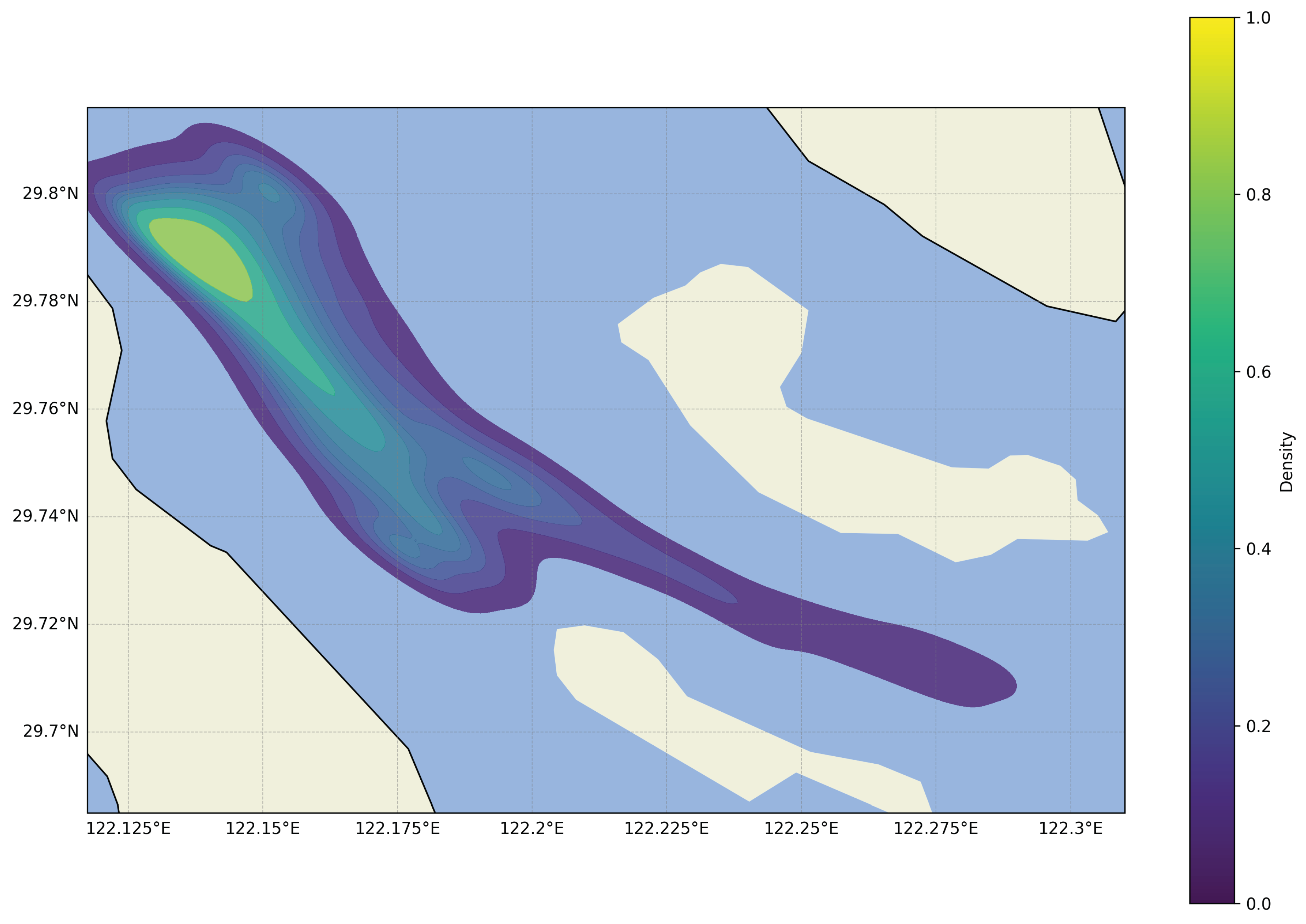
Figure 4.
This figure compares the original ship trajectory with the cubic spline-interpolated path in latitude-longitude space.
Figure 4.
This figure compares the original ship trajectory with the cubic spline-interpolated path in latitude-longitude space.
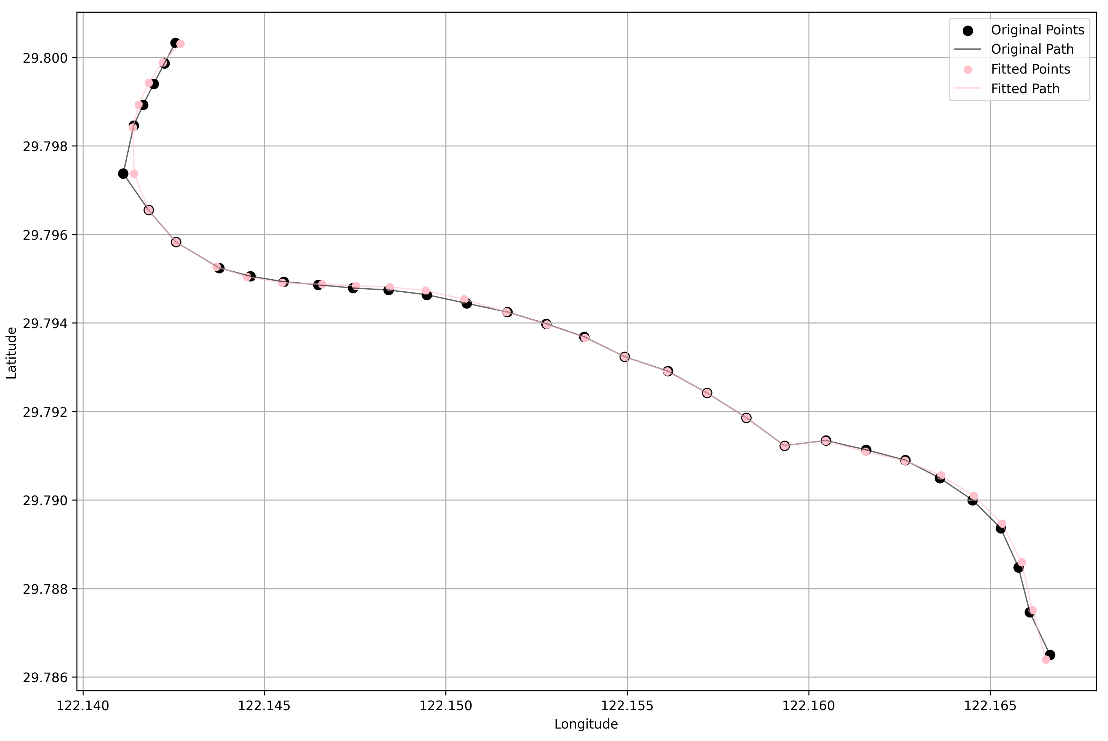
Figure 5.
After data augmentation of AIS points with large intervals by the difference method, the actual point and the predicted point are within a reasonable error range. The X-axis represents the timestamp (kilo second) and the Y-axis represents the error distance (kilo Nautical Mile).
Figure 5.
After data augmentation of AIS points with large intervals by the difference method, the actual point and the predicted point are within a reasonable error range. The X-axis represents the timestamp (kilo second) and the Y-axis represents the error distance (kilo Nautical Mile).
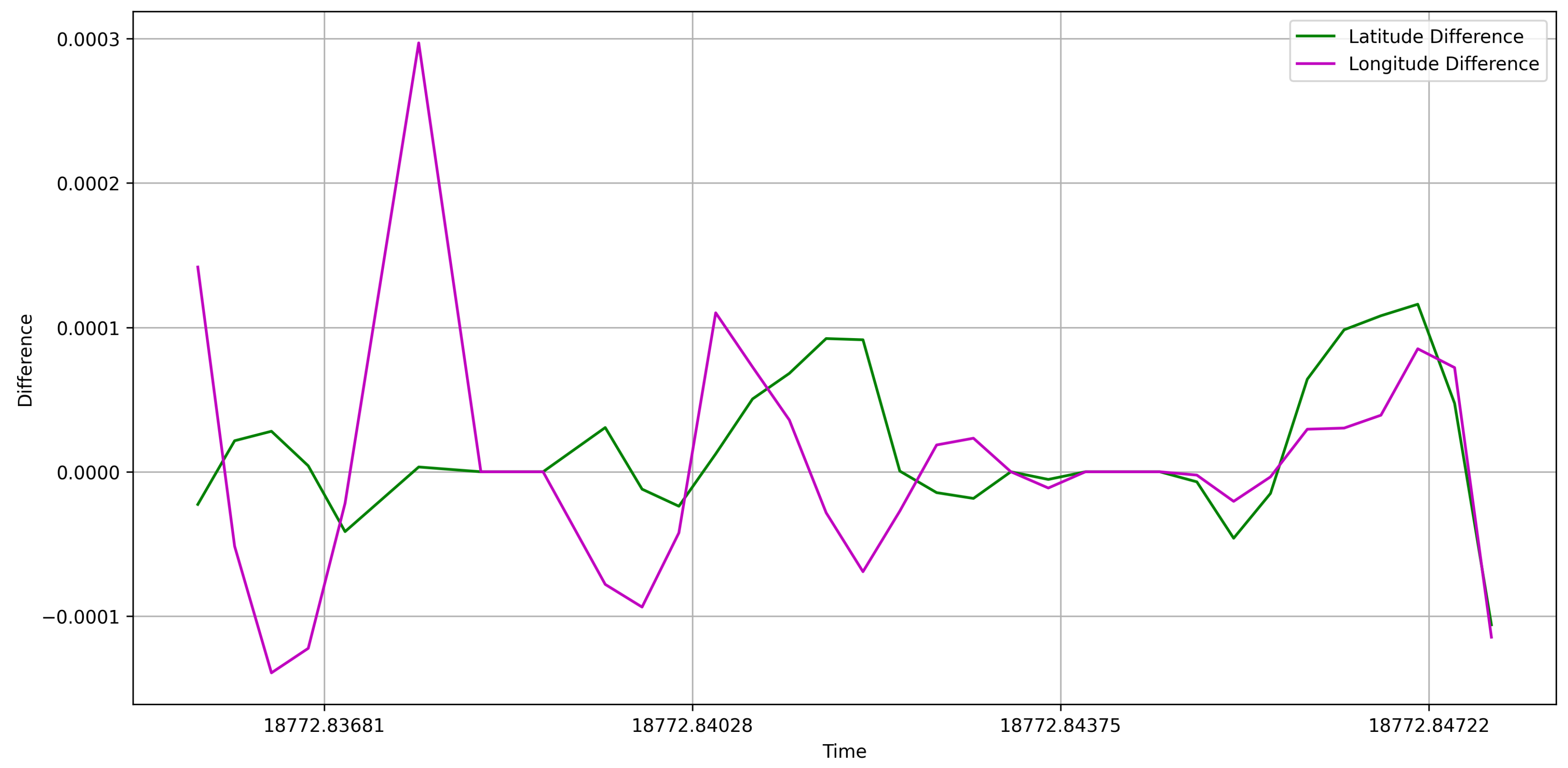
Figure 6.
Overall Structure of Exceptional Moving Average Attention.
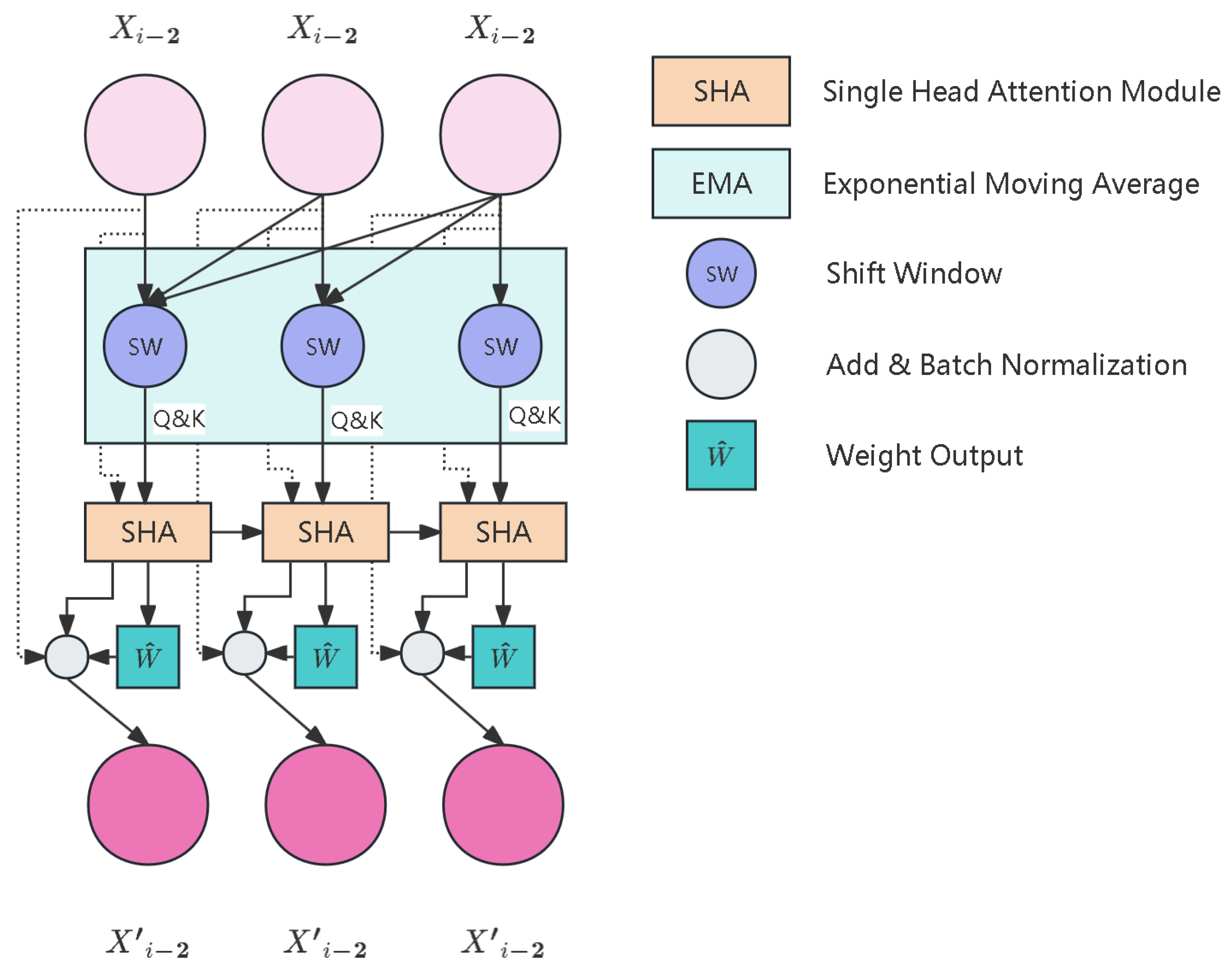
Figure 7.
The interpretation of SMA when the shift window size is 3.
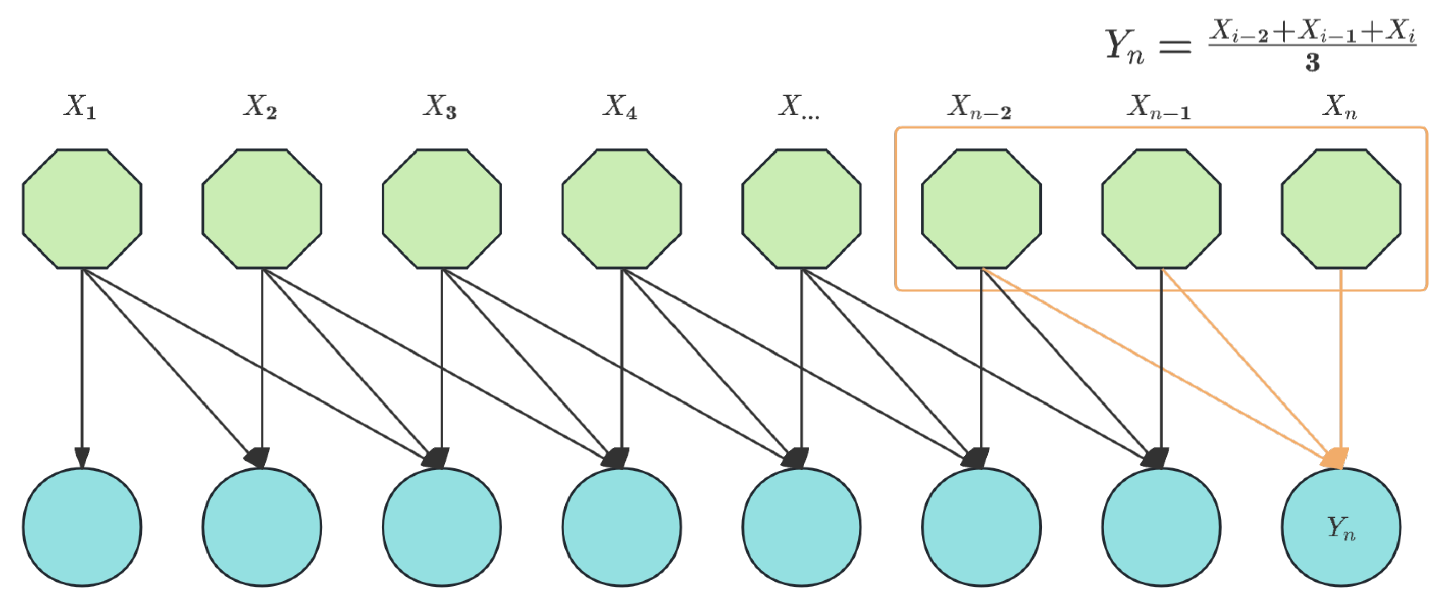
Figure 8.
The interpretation of WMA when the shift window size is 3.
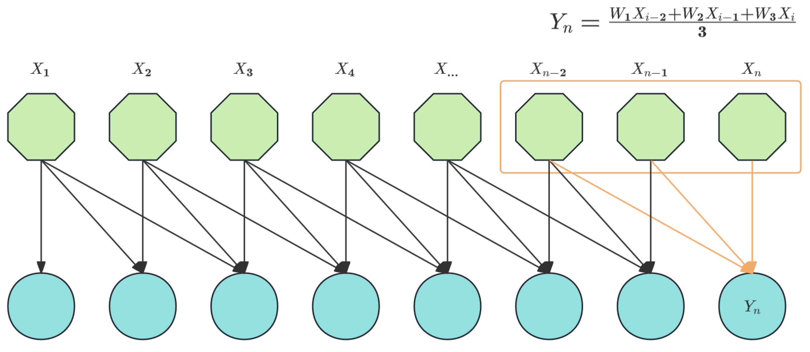
Figure 9.
The interpretation of CMA when the shift window size is 3.
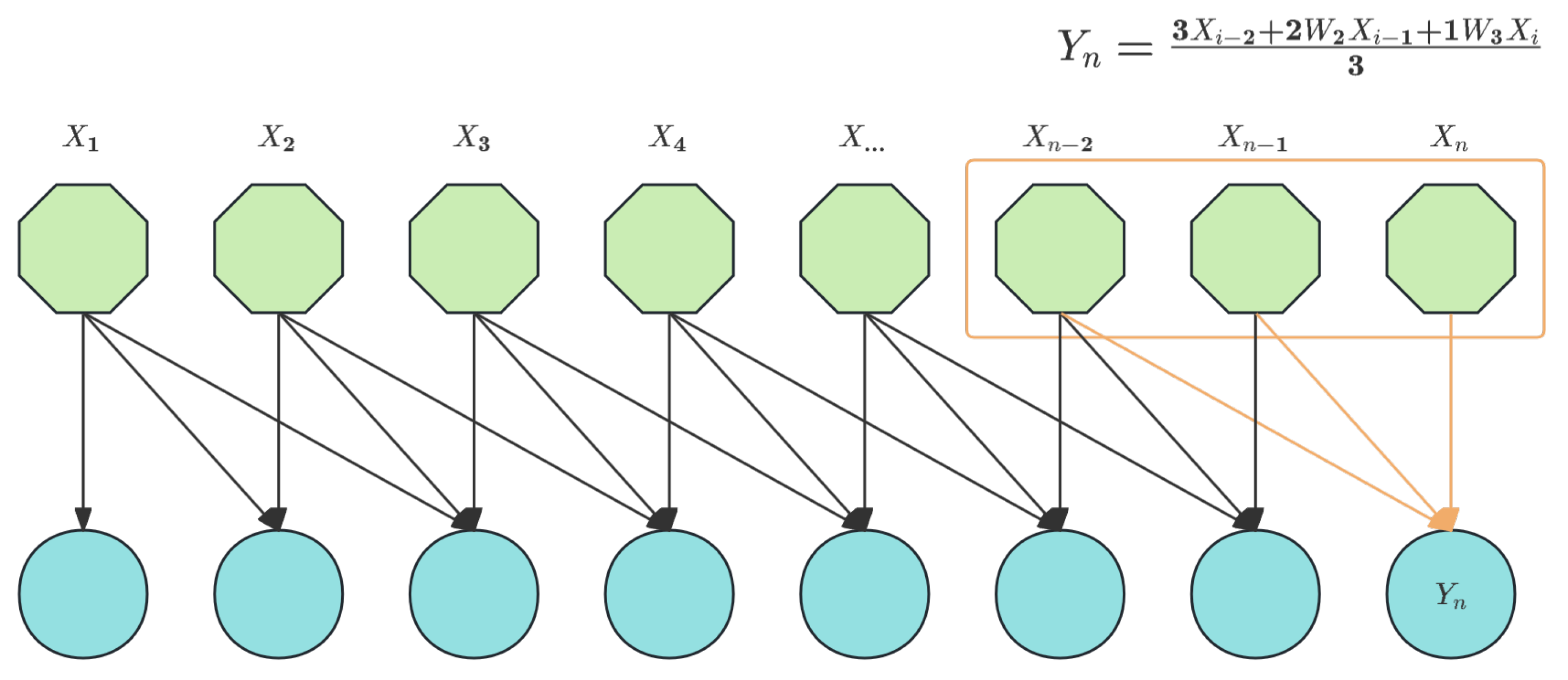
Figure 10.
The interpretation of EMA when the shift window size is 3.
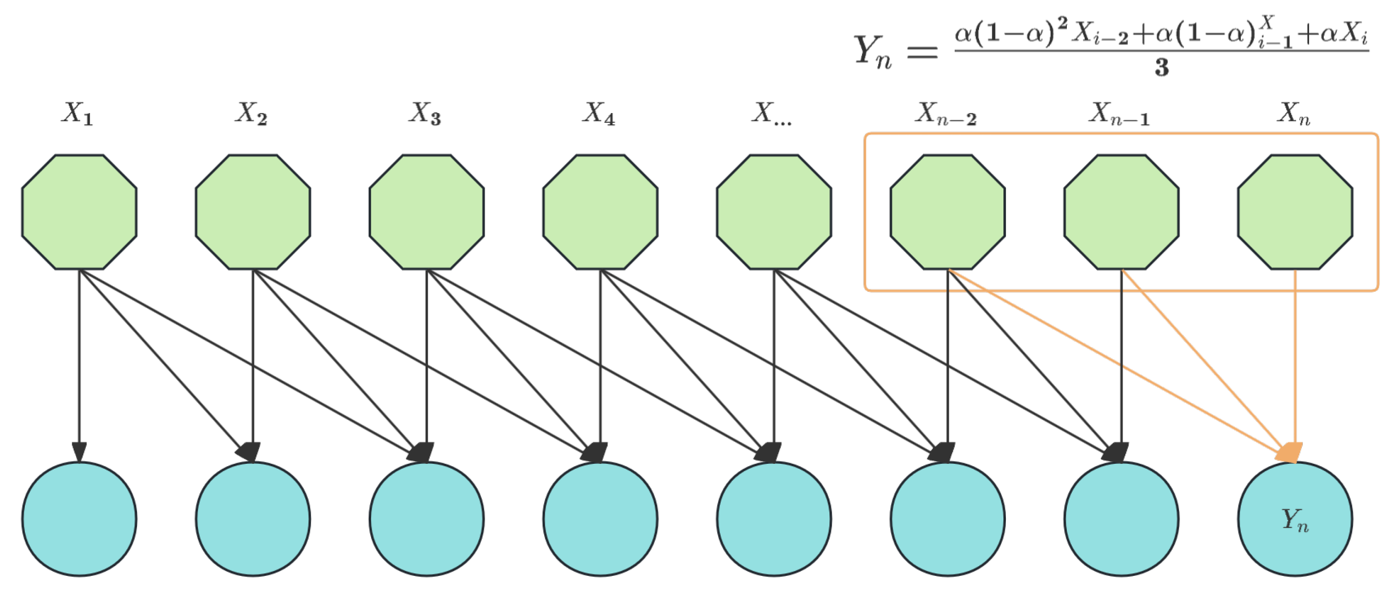
Figure 11.
Shift window single-head attention mechanism module. In this sample, the shift window of 3 is continued to be used as the reference.
Figure 11.
Shift window single-head attention mechanism module. In this sample, the shift window of 3 is continued to be used as the reference.
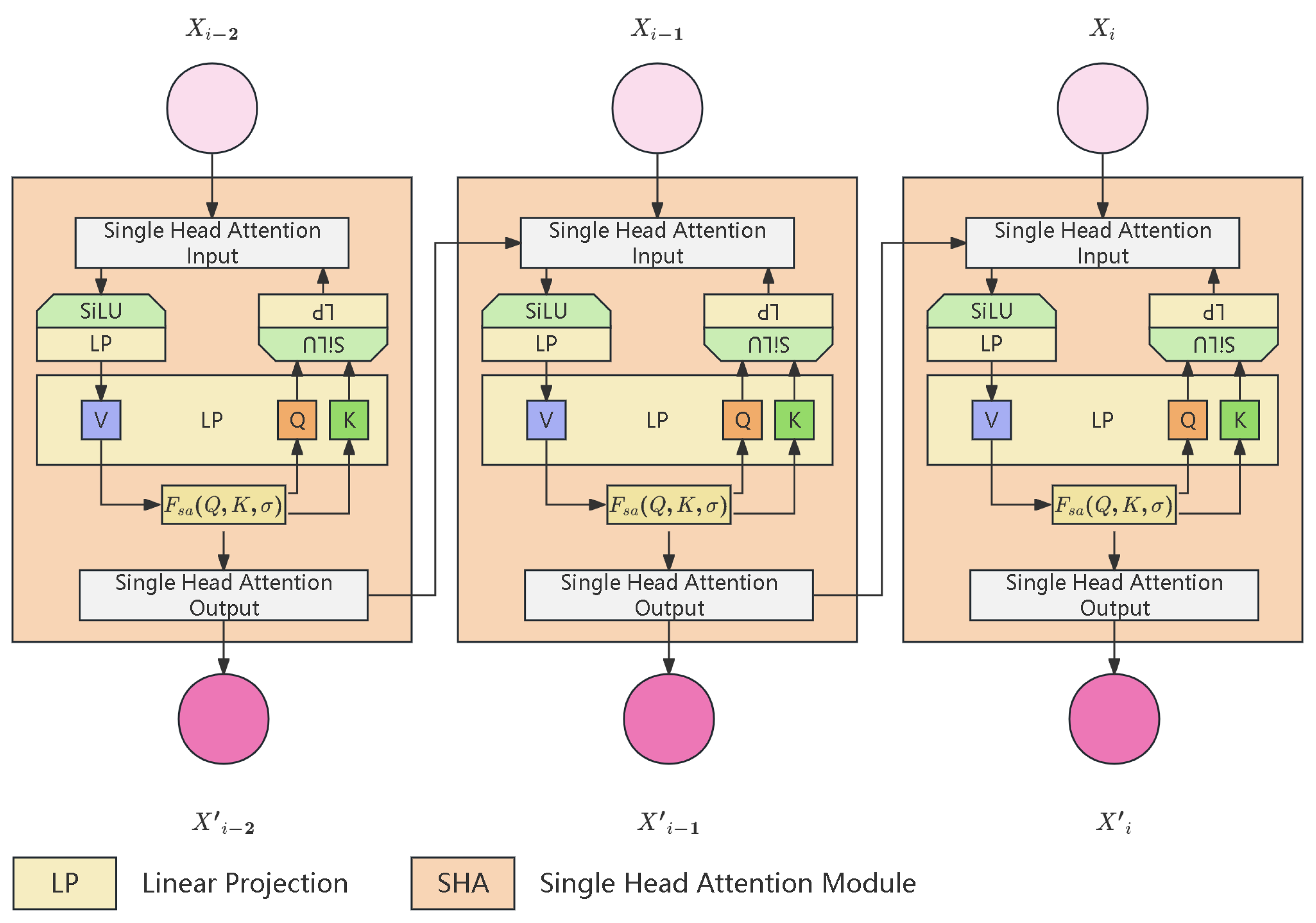
Figure 12.
The Overall Structure of State Space Models.
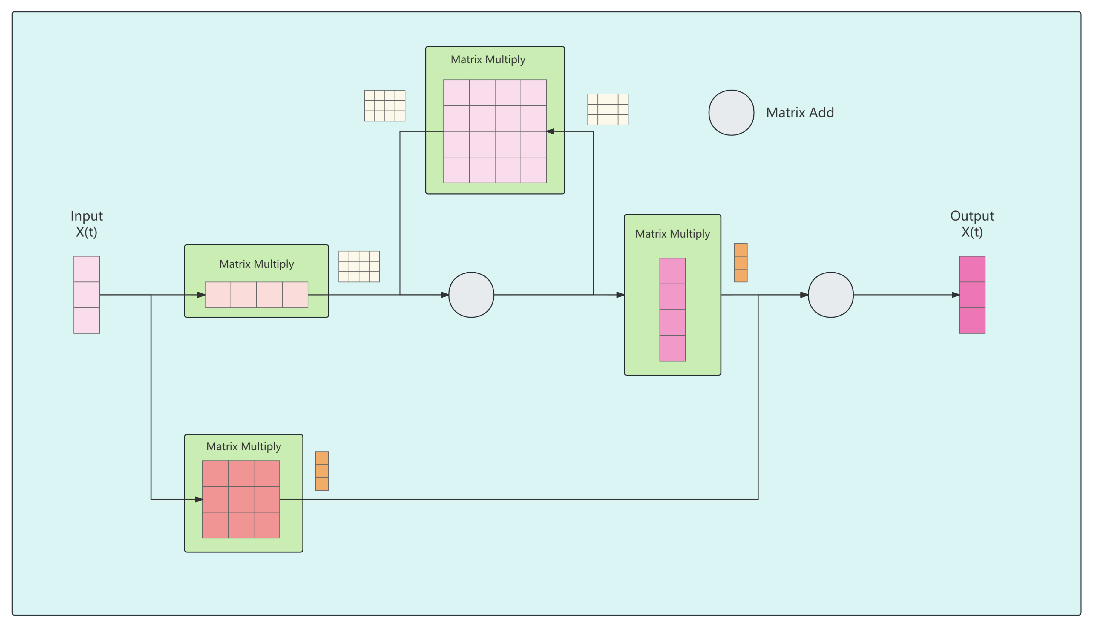

Table 1.
Performance comparison of different approaches
| Model | Class F1-Score | Macro Avg | Weighted Avg | ||||||||
|---|---|---|---|---|---|---|---|---|---|---|---|
| 0 | 1 | 2 | 3 | 4 | Prec | Rec | F1 | Prec | Rec | F1 | |
| Machine Learning | |||||||||||
| LGBM [31] | 0.54 | 0.52 | 0.49 | 0.47 | 0.64 | 0.66 | 0.51 | 0.53 | 0.64 | 0.53 | 0.53 |
| XGB [32] | 0.54 | 0.53 | 0.49 | 0.47 | 0.62 | 0.65 | 0.51 | 0.53 | 0.63 | 0.53 | 0.53 |
| RandomForest [33] | 0.54 | 0.50 | 0.48 | 0.45 | 0.58 | 0.55 | 0.50 | 0.51 | 0.54 | 0.52 | 0.51 |
| ExtraTrees [34] | 0.55 | 0.50 | 0.48 | 0.45 | 0.57 | 0.55 | 0.50 | 0.51 | 0.54 | 0.52 | 0.51 |
| KNeighbors [35] | 0.53 | 0.49 | 0.50 | 0.46 | 0.50 | 0.53 | 0.49 | 0.50 | 0.52 | 0.50 | 0.50 |
| Bagging [36] | 0.54 | 0.50 | 0.46 | 0.45 | 0.57 | 0.53 | 0.50 | 0.50 | 0.53 | 0.51 | 0.50 |
| ExtraTree [34] | 0.53 | 0.49 | 0.49 | 0.45 | 0.55 | 0.53 | 0.50 | 0.50 | 0.53 | 0.51 | 0.50 |
| DecisionTree [37] | 0.53 | 0.49 | 0.45 | 0.44 | 0.55 | 0.52 | 0.49 | 0.49 | 0.51 | 0.50 | 0.50 |
| Deep Learning | |||||||||||
| LSTM [22] | 0.78 | 0.61 | 0.50 | 0.56 | 0.75 | 0.65 | 0.65 | 0.64 | 0.65 | 0.66 | 0.65 |
| BiLSTM [38] | 0.94 | 0.49 | 0.45 | 0.48 | 0.86 | 0.68 | 0.64 | 0.64 | 0.70 | 0.66 | 0.66 |
| Transformer [39] | 0.61 | 0.38 | 0.16 | 0.36 | 0.65 | 0.52 | 0.47 | 0.43 | 0.52 | 0.49 | 0.44 |
| EMA [40] | 0.94 | 0.51 | 0.46 | 0.50 | 0.88 | 0.67 | 0.65 | 0.66 | 0.69 | 0.67 | 0.68 |
| SSM [41] | 0.75 | 0.64 | 0.53 | 0.57 | 0.77 | 0.47 | 0.47 | 0.47 | 0.66 | 0.67 | 0.66 |
| Ours | 0.94 | 0.71 | 0.55 | 0.65 | 0.90 | 0.79 | 0.76 | 0.75 | 0.80 | 0.77 | 0.76 |
| Class labels 0 to 4 represent the patterns: Normal, Cycle, U-turn, Detour, and Noise Cluster. | |||||||||||
Table 2.
Ablation experiment.
| No. | BS | Attention | SSM | Metric | |||||
|---|---|---|---|---|---|---|---|---|---|
| macro avg | weighted avg | ||||||||
| P | R | F1 | P | R | F1 | ||||
| 1 | LSTM | 0.6462 | 0.6469 | 0.6387 | 0.6543 | 0.6563 | 0.6478 | ||
| 2 | Mulit-Head | 0.5545 | 0.548 | 0.5454 | 0.5548 | 0.5449 | 0.5441 | ||
| 3 | EMA | 0.6677 | 0.6534 | 0.6586 | 0.6908 | 0.6716 | 0.6794 | ||
| 4 | Base | 0.4740 | 0.4690 | 0.4658 | 0.6643 | 0.6669 | 0.6576 | ||
| 5 | Gated | 0.6406 | 0.6261 | 0.6242 | 0.6653 | 0.6522 | 0.6497 | ||
| 6 | EMA | Base | 0.7274 | 0.7098 | 0.7043 | 0.7510 | 0.7176 | 0.7219 | |
| Ours | EMA | Gated | 0.7877 | 0.7557 | 0.7492 | 0.7996 | 0.7657 | 0.7610 | |
Disclaimer/Publisher’s Note: The statements, opinions and data contained in all publications are solely those of the individual author(s) and contributor(s) and not of MDPI and/or the editor(s). MDPI and/or the editor(s) disclaim responsibility for any injury to people or property resulting from any ideas, methods, instructions or products referred to in the content. |
© 2025 by the authors. Licensee MDPI, Basel, Switzerland. This article is an open access article distributed under the terms and conditions of the Creative Commons Attribution (CC BY) license (http://creativecommons.org/licenses/by/4.0/).
Copyright: This open access article is published under a Creative Commons CC BY 4.0 license, which permit the free download, distribution, and reuse, provided that the author and preprint are cited in any reuse.


