
Submitted:
13 May 2025
Posted:
14 May 2025
You are already at the latest version
Abstract
The paper describes two schemes, together with architectures, for the resource-efficient parallel computation of twiddle factors for the fixed-radix version of the fast Fourier transform (FFT) algorithm. Assuming a silicon-based hardware implementation with suitably chosen parallel computing equipment, the two schemes considered provide one with the facility for trading off the arithmetic component of the resource requirements, as expressed in terms of the numbers of multipliers and adders, against the memory component, as expressed in terms of the amount of memory required for constructing the look-up tables (LUTs) needed for their storage. With a separate processing element (PE) being assigned to the computation of each twiddle factor, the first scheme is based upon the adoption of the single‑instruction multiple‑data (SIMD) technique, as applied in the ‘spatial’ domain, whereby the PEs operate independently upon their own individual LUTs and may thus be executed simultaneously; the second scheme is based upon the adoption of the pipelining technique, as applied in the ‘temporal’ domain, whereby the operation of all but the first LUT-based PE is based upon second-order recursion using previously computed PE outputs. Although the FFT radix and LUT level (where the LUT may be of either single‑level or multi‑level type) may each take on arbitrary integer values, we will be particularly concerned with the radix-4 version of the FFT algorithm, together with the two‑level version of the LUT, as these two algorithmic choices facilitate ease of illustration and offer the potential for flexible computationally-efficient FFT designs. A brief comparison of the resource requirements for the two schemes is provided for various parameter sets which cater, in particular, for those big‑data memory-intensive applications involving the use of long (with length of order one million) to ultra-long (with length of order one billion) FFTs.
Keywords:
butterfly
; FFT
; LUT
; parallel
; recursion
; twiddle factor
1. Introduction
The discrete Fourier transform (DFT) is an orthogonal transform [1] which, for the case of N input/output samples, may be expressed in normalized form via the equation
where the input/output data vectors belong to CN, the linear space of complex-valued N-tuples, and the transform kernel is expressed in terms of powers of WN, where
the primitive Nth complex root of unity [3,15]. Fast solutions to the DFT are referred to generically as fast Fourier transform (FFT) algorithms [4-6] and, when the transform length is expressible as some power of a fixed integer R – whereby the algorithm is referred to as a fixed-radix FFT with radix R – enable the associated arithmetic complexity to be reduced from to just .
The complex-valued exponential terms, , appearing in Eqtn. 1, each comprise two trigonometric components – with each pair being more commonly referred to as twiddle factors [4-6] – that are required to be fed to each instance of the FFT’s butterfly, this being the computational engine used for carrying out the algorithm’s repetitive arithmetic operations and which, for a radix-R transform, produces R complex-valued outputs from R complex-valued inputs.
The twiddle factor requirement, more exactly, is that for a radix-R FFT algorithm there will be R-1 non-trivial twiddle factors to be applied to each butterfly. For a decimation-in-time (DIT) type FFT design [4-6], with typically digit-reverse (DR) -ordered inputs and naturally (NAT) -ordered outputs, the twiddle factors are applied to the butterfly inputs – see Figure 1, whilst for a decimation-in-frequency (DIF) type FFT design [4-6], with typically NAT-ordered inputs and DR-ordered outputs, the twiddle factors are applied to the butterfly outputs – see Figure 2. Each twiddle factor, as stated above, possesses two components, one being defined by the sine function and the other by the cosine function, which may be retrieved directly from the coefficient memory or generated on-the-fly in order to be able to carry out the necessary processing for the FFT butterfly.
Note that the DR-ordered and NAT-ordered index mappings referred to above may each be applied to either the input or output data sets for both the DIT and DIF variations of the fixed-radix FFT, yielding a total of four possible combinations for any fixed-radix transform: namely, DITNR, DITRN, DIFNR and DIFRN where ‘N’ refers to the NAT-ordered mapping and ‘R’ to the DR-ordered mapping and where the first letter of each pair corresponds to the input data mapping and the second letter to the output data mapping [5]. The DITRN and DIFNR radix-4 butterflies correspond to those already illustrated in Figs. 1 and 2, respectively, from which one can easily visualize how the designs may be straightforwardly generalized to higher radices. For the case of an arbitrary radix-R DIT algorithm, for example, the twiddle factors will be applied to all but one of the R butterfly inputs, whereas with the corresponding DIF algorithm, the twiddle factors will be applied to all but one of the R butterfly outputs.
When the DFT is viewed as a matrix operator, Eqtn. 1 becomes a matrix-vector product, with the effect of the radix-R FFT being to factorize the N×N DFT matrix into a product of logRN sparse matrices, with each sparse matrix being of size N×N and comprising N/R sub-matrices, each of size R×R, where each sub-matrix corresponds in turn to the operation of a radix-R butterfly. Thus, each sparse matrix factor produces N partial-DFT outputs though the execution of N/R radix-R butterflies. The effect of such a factorization is thus to reduce the computation of the original length-N transform to the execution of logRN computational stages, with each stage comprising radix-R butterflies, where the execution of a given stage can only commence once that of its predecessor has been completed, and with the FFT output being produced on completion of the final computational stage. Thus, from this analysis, it is evident that the computational efficiency of the fixed-radix FFT is totally dependent upon the computational efficiency of the individual butterfly.
Also, an efficient parallel implementation of the fixed-radix FFT – particularly for the processing of long (of order one million samples, as might be encountered with the processing of wideband signals embedded in astronomical data) to ultra-long (of order one billion samples, as might be encountered with the processing of ultra-wideband signals embedded in cosmic microwave data) data sets [13] – invariably requires an efficient parallel mechanism for the generation or computation of the twiddle factors (unless the DFT is solved by approximate means via the adoption of a suitably defined sparse FFT algorithm [8,11]) as it is essential that the full set of R-1 non-trivial terms required by each radix-R butterfly – whether applied to the inputs or the outputs – should be available simultaneously in order to avoid potential timing issues and delays and to be produced at a rate that is consistent with the processing rate of the FFT.
The computational efficiency of the twiddle factor generation for the fixed-radix FFT may be optimized by trading off the arithmetic component of the resource requirement against the memory component through the combined use of appropriately defined look-up tables (LUTs) – which may be of either single-level (comprising a single LUT with a fixed angular resolution) or multi-level (comprising multiple single-level LUTs each with its own distinct fixed angular resolution) type [10,12] – and trigonometric identities. Although the FFT radix can actually take on any integer value, the most commonly used radices are those of two and four, primarily for the resulting flexibility (generating a large number of possible transform sizes for various possible applications) that they offer and for ease of implementation. The attraction of choosing a solution based upon the radix-4 factorization, rather than that of the more familiar radix-2, is that of its greater computational efficiency – in terms of both a reduced arithmetic requirement (that is, of the required numbers of multiplications and additions) and reduced number of memory accesses (four complex-valued samples at a time instead of just two – comprising both real and imaginary components) for the retrieval of data from memory.
There is, in turn, the potential for exploiting greater parallelism, at the arithmetic level, via the use of a larger sized butterfly, thereby offering the possibility of achieving a higher computational density (that is, throughput per unit area of silicon [9]) when implemented in silicon with a suitably chosen computing device and architecture. As a result, we will be particularly concerned with the radix-4 version of the FFT algorithm, together with the two-level version of the LUT, as these two algorithmic choices facilitate ease of illustration and offer the potential for flexible computationally-efficient FFT designs.
Thus, following this introductory section, complexity considerations for both sequential and parallel computing devices are discussed in Section 2, followed by the derivation of a collection of formulae in Section 3 for some of the standard trigonometric identities which, together with suitably defined LUTs – dealing with both single-level and multi-level types – as discussed in Section 4, will be required for the efficient computation of the twiddle factors. Section 5 then describes, in some detail, two different parallel computing solutions to the task of twiddle factor computation where the computation of each twiddle factor is assigned its own processing element (PE). The first scheme is based upon the adoption of the single- instruction multiple-data (SIMD) technique [2], as applied in the spatial domain, whereby the PEs operate independently upon their own individual LUTs and may thus be executed simultaneously, whilst the second scheme is based upon the adoption of the pipelining technique [2], as applied in the temporal domain, whereby the operation of all but the first LUT-based PE is based upon second-order recursion using previously computed PE outputs. Detailed examples for these two approaches are provided using a radix-4 butterfly combined with two-level LUTs and a brief comparative analysis provided in terms of both the space-complexity, as expressed in terms of their relative arithmetic and memory components, and the time-complexity, as expressed in terms of their associated latencies and throughputs, for a silicon-based hardware implementation. Finally, a brief summary and conclusions is provided in Section 6.
2. Complexity Considerations
When dealing with questions of complexity relating to the twiddle factor computations for the case of a sequential single-processor computing device, as is the case in Section 3 and Section 4, the memory requirement is to be denoted by CMEM, with the associated arithmetic complexity being referred to via the required number of arithmetic operations, as expressed in terms of the number of multiplications, denoted CMPY, and the number of additions/subtractions, denoted CADD. When dealing with a silicon-based hardware implementation, however, on a suitably chosen parallel computing device – as might typically be made available with field- programmable gate array (FPGA) technology [14] – the complexity is to be defined in terms of the space-complexity and time-complexity. These parallel computing aspects, as will be discussed in some detail in Section 5, will be the main focus of our interest
The space-complexity comprises: 1) the memory component, denoted RMEM, (and which is the same as CMEM when expressed in ‘words’) which represents the amount of random access memory (RAM) needed for construction of the LUTs; and 2) the arithmetic component, which consists of the number of arithmetic operators, as expressed in terms of the number of hardware multipliers, denoted RMPY, and the number of hardware adders, denoted RADD, assigned to the computational task. Note also, that with the adoption of fixed-point arithmetic, multiplication by any power of two equates to that of a simple left-shift operation, with multiplication by two thereby equating to that of a left-shift operation of length just one. The associated time-complexity will be represented by means of the latency, which is the elapsed time between the initial accesses of trigonometric data from an LUT to the production of the corresponding twiddle factor, and the throughput rate, which is the number of twiddle factors that can be produced in a given period of time (typically taken to be a clock cycle, which is the rate at which the target computing device operates).
3. Schemes Based Upon Second-Order Recursion
The radix-4 FFT butterfly, which from Figs. 1 and 2 operates on four complex-valued inputs to produce four complex-valued outputs, requires the additional input of four complex-valued twiddle factors where the first twiddle factor is trivial with a fixed value of one and the remaining three non-trivial twiddle factors take on values of and for some given value of ‘θ’ – noting that the cosine terms correspond to the ‘real’ component and the sine terms to the ‘imaginary’ component. These three pairs of trigonometric terms are also those required by the large double-sized butterfly of the regularized version of the fast Hartley transform (FHT), which has strong connections to the real-data version of the radix-4 FFT, as discussed in some detail in [9]. A key task, therefore, is to show how such terms may be efficiently obtained, either 1) from the contents of one or more two-level LUTs – where such LUTs will be described in some detail in Section 4 – with the two sets of trigonometric outputs being subsequently combined via the standard two-angle identity, or 2) obtained directly, in a recursive manner, from previously computed twiddle factors via the application of suitably defined multi-angle formulae.
3.1. Standard Two-Angle Identity
The relevant trigonometric formulae required for addressing this task may be derived in a straightforward manner from the standard two-angle identities
where, when dealing with the case of the two-level LUT, ‘’ may be viewed as corresponding to the angle defined over a coarse-resolution angular region and ‘’ to the angle defined over a fine-resolution angular region – see the simplified illustration of Figure 3 for the decomposition of the cosine function into coarse-resolution and fine-resolution angular regions, each of length four. The total arithmetic complexity associated with the two-angle formulae is thus given by
CMPY = 4 & CADD = 2
3.2. Derivation of Double-Angle Formulae
The most simple of the non-trivial trigonometric expressions required for the twiddle factor computation of the radix-4 butterfly – when obtained directly via the application of trigonometric identities – are those of the double-angle formulae, as obtained by setting equal to θ in Eqtns. 3 and 4, and given by
which may also be expressed as
Thus, the total arithmetic complexity associated with the double-angle formulae is given by
where each trigonometric multiplication (that is, involving two trigonometric terms) is followed by a simple left-shift operation of length one.
CMPY = 2 & CADD = 1
3.3. Derivation of Triple-Angle Formulae
The most complex of the non-trivial trigonometric expressions required for the twiddle factor computation of the radix-4 butterfly – when obtained directly via the application of trigonometric identities – are those of the triple-angle formulae, as obtained by setting equal to 2θ in Eqtns. 3 and 4, and given by
Thus, the total arithmetic complexity associated with the triple-angle formulae is given by
where each trigonometric multiplication is again followed by that of a simple left-shift operation of length one.
CMPY = 2 & CADD = 2
3.4. Generalization to Multi-Angle Formulae
The expressions given by Eqtns. 6, 7, 10 and 11 correspond to those required for the non-trivial twiddle factor computation of the two largest angles for the radix-4 butterfly. It is clearly possible, however, without too much difficulty, to generalize these results to yield arbitrary multi-angle recursive formulae, as given by
where ‘n’ is an arbitrary positive integer > 1. Thus, as for the triple-angle case, the total arithmetic complexity associated with the multi-angle formulae is given by
where each trigonometric multiplication is again followed by that of a simple left-shift operation of length one.
CMPY = 2 & CADD = 2
3.5. Discussion
Note that Eqtns. 13 and 14 given above, which are both recursive equations of order two – each being commonly referred to as a second-order recursion or recurrence relation – clearly correspond to those needed for the twiddle factor computation of any radix-R butterfly, where R > n, when they are to be obtained directly from previously computed twiddle factors, rather than from a suitably defined LUT. The computation of each twiddle factor is thus clearly dominated by the need to perform two trigonometric multiplications, where each such multiplication is followed by that of a simple left shift operation, of length one, followed by that of a subtraction.
4. Schemes Based Upon Multi-Level LUTs
The efficient implementation of the fixed-radix butterfly invariably requires an efficient mechanism for the computation of the twiddle factors, particularly when dealing with long to ultra-long transforms. The total size of memory required by the LUT(s), as needed for their storage, can be minimized by exploiting the relationship between the cosine and sine functions, as given by the expression
as well as the periodic nature of each, as given by the expressions
Schemes are now outlined which enable a simple trade-off to be made between memory size and addressing complexity, as measured in terms of the number of arithmetic operations required for computing the necessary memory addresses.
4.1. Derivation of Single-Level LUT-Based Scheme
For the case of the radix-4 FFT butterfly the non-trivial twiddle factors comprise both cosinusoidal and sinusoidal terms for single-angle, double-angle and triple-angle cases. To minimize the arithmetic complexity for the generation of the addresses, the LUT is best sized according to a single-quadrant addressing scheme [12], whereby the twiddle factors are read from a sampled version of the sine (or, equivalently, cosine) function with argument defined from 0 up to radians. As a result, each LUT may be accessed by means of a single, easy to compute, input parameter which may be updated from one access to another via simple addition using a fixed increment – that is, the addresses form an arithmetic sequence. Thus, for the case of an N-point transform, it is required that the LUT be of length N/4, yielding a total memory requirement of
words, with the associated arithmetic complexity, as expressed in terms of the required numbers of multiplications and additions, per twiddle factor, being given by
respectively – that is, two additions for the computation of each twiddle factor, one for the LUT address of the sinusoidal component and one for that of the cosinusoidal component. This single-level scheme [12] described here would seem to offer, therefore, a reasonable compromise between the memory requirement and the addressing complexity, using more than the minimum achievable amount of memory required for the storage of the twiddle factors (albeit considerably less than would be required if the full 0 to 2π angular range was to be tabulated) so as to keep the arithmetic complexity of the addressing as simple as possible.
4.2. Derivation of Two-Level LUT-Based Scheme
The two-level case described here comprises one coarse-resolution angular region of length N/4L for the sine (or, equivalently, cosine) function, covering 0 up to radians, and one fine-resolution angular region of length L for each of the cosine and sine functions, covering 0 up to radians. The required twiddle factors may then be obtained from the contents of the two-level LUT through the application of one or other of the standard trigonometric identities, as given by Eqtns. 3 and 4.
By expressing the combined size – representing the total number of distinct angles – of the two-level LUT for the sine function as having to cater for
words, it can be seen via the straightforward application of the differential calculus [7] that the optimum single-level LUT length is obtained when the derivative
is set to zero, giving and resulting in a total memory requirement for this two-level scheme [12] of
words – for the coarse-resolution angular region (as required by the sine or cosine function) and for each of the two fine-resolution angular regions (as required by both the sine and cosine functions). This memory requirement, although clearly lower than that of the single-level scheme, is achieved at the expense of an increased arithmetic complexity, per twiddle factor, namely
where four of the additions are for generating the LUT addresses – that is, two to cater for both the sine and cosine functions defined over the coarse-resolution region and two to cater for the sine and cosine functions, one per LUT, defined over the fine-resolution region.
4.3. Generalization to Multi-Level LUT-Based Scheme
Finally, the results obtained for the two-level scheme may be straightforwardly extended to the general case of an arbitrary K-level scheme, where K ≥ 2. By expressing the combined size of the K-level LUT for the sine function as having to cater for
words, where the LUTs are assumed for ease of analysis to be each of length L, it can be seen that the optimum single-level LUT length is obtained when the derivative
is set to zero, giving
(since K > 1) and resulting in a total memory requirement for this multi-level scheme [12] of
words – that is, to cater for both the sine and cosine functions defined over the coarse-resolution region and to cater for each of the sine and cosine functions defined over each of the K-1 fine-resolution regions. The computational cost per twiddle factor, however, for K ≥ 2, would increase to
where 2K of the additions are for generating the LUT addresses – that is, two to cater for both the sine and cosine functions defined over the coarse-resolution region and two to cater for the sine and cosine functions, one per LUT, defined over each of the K-1 fine-resolution regions.
4.4. Discussion
To illustrate the trade-off of arithmetic complexity against memory requirement, per twiddle factor, for both the single-level and multi-level schemes, a set of results is provided in Table 1 which deal with a range of FFT lengths: one binary thousand (or 210=1024), one binary million (or 220=1,048,576), and one binary billion (or 230=1,073,741,824), which may be regarded as close approximations to one thousand (or 103=1,000), one million (or 106=1,000,000), and one billion (or 109=1,000,000,000), respectively, and which may each be tackled with a suitably defined radix-2K algorithm. Note that the last column of Table 1 indicates how many independent tasks are required for carrying out each of the LUT-based schemes, as this parameter will determine how well each of the schemes will parallelize and therefore map onto silicon-based hardware – as will be discussed next in Section 5.
5. Parallel Computation of Twiddle Factors
Two parallel schemes, together with architectures, are now described for the computation of the twiddle factors for the radix-4 FFT butterfly, assuming the adoption of a suitably chosen parallel computing device. The space-complexity is first discussed, whereby one is able to optimize the resource utilization by trading off the memory component against the arithmetic component. The time-complexity is also discussed, this relating to how the two approaches may differ in terms of latency, due to possible timing delays, and throughput, due to possible differences in the computational needs of their respective PEs. The requirement, for a fully parallel implementation of the radix-4 FFT, is that all the twiddle factors are to be made simultaneously available for input to each instance of the radix-4 butterfly, thereby preventing potential timing delays and enabling the associated butterfly and its FFT to achieve and maintain real-time operation.
There are two computational domains where parallelism may be exploited: namely, the temporal domain and the spatial domain. The first of the two proposed schemes is based upon the adoption of the SIMD technique, as applied in the spatial domain, whilst the second is based upon the adoption of the pipelining technique, as applied in the temporal domain. Both approaches use one or more two-level LUTs, where the contents of a given LUT are combined in an appropriate fashion via the standard two-angle identities of Eqtns. 3 and 4 – as illustrated in Figure 4.
5.1. SIMD Approach with Multiple LUTs
With the SIMD approach, the computation of each non-trivial twiddle factor is assigned its own PE which has access, in turn, to its own individual two-level LUT, as illustrated in Figure 5, thereby enabling each PE to produce a twiddle factor via the application of the standard two-angle identities of Eqtns. 3 and 4. As the parallelism is defined in the spatial domain, all three PEs may operate independently, being thus able to produce all three non-trivial twiddle factors simultaneously – noting that the other remaining twiddle factor is trivial with a fixed value of one. As a result, all the non-trivial twiddle factors are available for input to the radix-4 butterfly at the same time.
By denoting by the logic-based function that converts a pair of angles, and , to the required set of addresses for accessing the two-level LUT, the initial operation of the PEs may be defined in the following way:
where addresses m1 and m2 both access the coarse-resolution LUT, whilst addresses n1 and n2 each accesses its own fine-resolution LUT. The subscripts/superscripts ‘S’, ‘D’ and ‘T’ refer to the angles used by the single-angle, double-angle and triple-angle twiddle factors, respectively.
These addresses, together with the coarse-resolution LUT, denoted , and the two fine-resolution LUTs, denoted and , now enable the subsequent operation of the PEs to be defined in the following way:
so that, for a fully-parallel silicon-based hardware implementation, the execution of all three PEs require a total of: 1) 12 adders plus logic for setting up the three sets of LUT addresses, plus 2) 12 multipliers and six adders for the subsequent derivation of the twiddle factors, together with 3) three two-level LUTs, each two-level LUT comprising three single-level LUTs, each of length for the case of a length-N transform.
5.2. Pipelined Approach with One LUT + Recursion
With the pipelined approach, each non-trivial twiddle factor is again computed with its own PE, but whereas the first PE has access to its own individual two-level PE, the remaining two PEs each produce a twiddle factor in a recursive manner from the previously computed twiddle factors, as illustrated in Figure 6, via the application of the multi-angle formulae of Eqtns. 6 and 7 for the second non-trivial twiddle factor and Eqtns. 10 and 11 for the third non-trivial twiddle factor – these equations being particular cases of those expressed generically via Eqtns. 13 and 14. As the parallelism is defined in the temporal domain, the processing within each PE relies on the outputs produced by its predecessors, with the processing for a given PE being only able to commence once that of its predecessor has been completed. As a result, timing delays are required to ensure that all the non-trivial twiddle factors become available for input to the radix-4 butterfly at the same time – noting that the other remaining twiddle is trivial with a fixed value of one.
By denoting by the logic-based function that converts a pair of angles, and , to the required set of addresses for accessing the two-level LUT, the initial operation of the first PE may be defined in the following way:
and its subsequent operation as
The twiddle factor outputs from the remaining PEs are derived in a recursive manner from previously computed twiddle factors, so that if
they may be defined in the following way:
so that, for a fully-parallel silicon-based hardware implementation, the execution of all three PEs require a total of: 1) four adders plus logic for setting up the set of LUT addresses, plus 2) eight multipliers (four of which – as required for PE2 and PE3 – are followed by a left-shift operation of length one) and five adders for the subsequent derivation of the twiddle factors, together with 3) one two-level LUT, comprising three single-level LUTs, each of length for the case of a length-N transform.
5.3. Comparison of Resource Requirements
Firstly, from Section 5.1, the total space-complexity for the twiddle factor computation via the SIMD-based solution may be expressed in terms of its arithmetic and memory components, denoted TA and TM, respectively, where
together with a small amount of logic for the address generation, and
words, for the case of a length-N transform.
TA = 12 multipliers & 18 adders
Secondly, from Section 5.2, the total space-complexity for the twiddle factor computation via the pipelined solution may also be expressed in terms of its arithmetic and memory components, denoted TA and TM, respectively, where
together with four trivial left-shift operations, each of length one, and a small amount of additional logic for the address generation, and
words, for the case of a length-N transform.
TA = 8 multipliers & 9 adders
Assuming a silicon-based hardware implementation with a suitably chosen FPGA-based parallel computing device, the arithmetic component of the space-complexity of each solution will be dominated by the number of multipliers, given that for fixed-point arithmetic and with a word-length of W, the complexity of a multiplier will involve O(W2) slices of programmable logic whereas an adder will involve just O(W) such slices. As a result, the arithmetic component of the space-complexity for the pipelined solution is approximately two-thirds that of the SIMD-based solution, whilst its memory component is just one-third that of the SIMD-based solution, making the pipelined solution the more resource-efficient – and thus able to achieve a higher computational density – of the two studied solutions and particularly attractive, due to the low memory component, for those big-data memory-intensive applications involving the use of long to ultra-long FFTs.
Note that with both solutions, whilst the adders may be implemented very simply in programmable logic, optimal arithmetic efficiency will be obtained when the multiplications are carried out using the fast embedded multipliers as provided by the equipment manufacturer.
5.4. Discussion
To address the question of time-complexity for the two studied solutions, note firstly that the implementation of each LUT-based PE, as is evident from Eqtns. 36 to 41, involves the operation of four multipliers, which may be carried out in parallel, followed by the operation of two adders, which may also be carried out in parallel. For the remaining PEs, the twiddle factors are produced from previously computed twiddle factors in a recursive manner, so that the implementation of each such PE, as is evident from Eqtns. 47 to 50, involves the operation of just two multipliers, which may be carried out in parallel, followed by the operation of two adders, which may also be carried out in parallel. As a result, with simple internal pipelining for the implementation of the multipliers and adders, the computation for each type of PE would possess comparable latency with each PE able to produce a new twiddle factor every clock cycle. Therefore, with each type of solution, whether of SIMD or pipelined type, the set of three PEs could produce a new set of non-trivial twiddle factors every clock cycle and would thereby be consistent with the throughput rate of the associated butterfly – assuming the butterfly to be also implemented in a fully-parallel fashion using SIMD and/or pipelining techniques – thereby enabling the associated butterfly and its FFT to achieve and maintain real-time operation.
Thus, assuming the latency of each internally-pipelined PE to be one time step – expressible itself as a fixed number of clock cycles – then the only difference in time-complexity between parallel implementations of the radix-4 FFT, using the two types of twiddle factor computation schemes discussed, is that the pipelined solution requires an additional two time steps to account for the initial start-up delay due to the internal pipelining of PE2 and PE3.
Finally, note that although we have discussed the particular case of the radix-4 butterfly and its associated twiddle factors, the results generalize in a straightforward manner to the case of a radix of arbitrary size. Clearly, a radix-R butterfly would need the input of R-1 non-trivial twiddle factors, rather than the three discussed here. For the SIMD-based solution, the arithmetic and memory components of the space-complexity for the case of a length-N transform may be approximated by
and
words, whilst for the pipelined solution, the arithmetic and memory components of the space-complexity may be approximated by
and
words. As a result, the arithmetic component of the space-complexity for the pipelined solution is approximately (R-2)/(R-1) that of the SIMD-based solution, whilst its memory component is just 1/(R-1) that of the SIMD-based solution, making the two solutions comparable, for sufficiently large R, in terms of their arithmetic component, but with the pipelined solution being clearly increasingly more memory-efficient, with increasing R, and thus making it particularly attractive for those big-data memory-intensive applications involving the use of long to ultra-long FFTs.
TA = 4×(R-1) multipliers & 6×(R-1) adders
TA = 4×(R-2) multipliers & 2×R+1 adders
A comparison of the space-complexities for the two solutions, for various FFT radices and transform lengths, is provided in Table 2, whereby the relative attractions of the two schemes for different scenarios are evident. The larger FFT radices are included purely for the purposes of illustration and, although the amount of resources clearly increases with increasing radix, it is also the case that greater parallelism is achievable with the larger-sized butterfly so that the computational throughput may also be commensurately increased in terms of outputs per clock cycle. As one would expect, only the memory component of the space-complexity for the twiddle factor computation varies as the transform length is increased.
6. Summary and Conclusions
The paper has described two schemes, together with architectures, for the resource-efficient parallel computation of twiddle factors for the fixed-radix version of the FFT algorithm. Assuming a silicon-based hardware implementation with a suitably chosen parallel computing device, the two schemes have shown how the arithmetic component of the resource requirement, as expressed in terms of the numbers of hardware multipliers and adders, may be traded off against the memory component, as expressed in terms of the amount of RAM required for constructing the LUTs needed for their storage. Both schemes showed themselves able to achieve the throughputs needed for the associated butterfly and its FFT to achieve and maintain real-time operation.
The first scheme considered was based upon the adoption of the SIMD technique, as applied in the spatial domain, whereby the PEs operated independently upon their own individual LUTs and were thus able to be executed simultaneously, whilst the second scheme was based upon the adoption of the pipelining technique, as applied in the temporal domain, whereby the operation of all but the first LUT-based PE was based upon second-order recursion using previously computed PE outputs. Both schemes were assessed using the radix-4 version of the FFT algorithm, together with the two-level version of the LUT, as these two algorithmic choices facilitated ease of illustration and offered the potential for flexible computationally-efficient FFT designs – the attraction of the radix-4 butterfly being its simple design and low arithmetic complexity, with the attraction of the two-level LUT being a memory requirement of just , as opposed to the of the more commonly used single-level LUT, making it ideally suited to the task of minimizing the twiddle factor storage.
The study concluded with a brief comparative analysis of the resource requirements which showed that for the pipelined solution, the arithmetic component of the space-complexity was approximately two-thirds that of the SIMD-based solution, whilst its memory component was just one-third that of the SIMD-based solution, making the pipelined solution the more resource-efficient – and thus able to achieve a higher computational density – of the two studied solutions and particularly attractive, due to the low memory component, for those big-data memory-intensive applications involving the use of long to ultra-long FFTs.
Conflicts of Interest
The author declares no conflicts of interest relating to the production of this paper.
References
- N. Ahmed & K.R. Rao, “Orthogonal Transforms for Digital Signal Processing”, Springer, 2012.
- S.G. Akl, “The Design and Analysis of Parallel Algorithms”, Prentice-Hall, 1989.
- G. Birkhoff & S. MacLane, “A Survey of Modern Algebra”, Macmillan, 1977.
- E.O. Brigham, “The Fast Fourier Transform”, Prentice-Hall, 1974.
- E. Chu & A. George, “Inside the FFT Black Box: Serial and Parallel Fast Fourier Transform Algorithms”, CRC Press, 2000.
- D.F. Elliott & K. Ramamohan Rao, “Fast Transforms: Algorithms, Analyses, Applications”, Academic Press, 1982.
- G.H. Hardy, “A Course of Pure Mathematics”, Cambridge University Press, 1928.
- H. Hasssanieh, P. Indyk, D. Katabi & E. Price, “Simple and Practical Algorithm for Sparse Fourier Transform”, ACM-SIAM Symposium on Discrete Algorithms, Kyoto, Japan, pp. 1183-1194, 2012.
- K. Jones, “The Regularized Fast Hartley Transform: Low-Complexity Parallel Computation of the FHT in One and Multiple Dimensions”, 2nd Edition, Springer (Series on Signals & Communication Technology), 2022.
- K. Jones, “A Comparison of Two Recent Approaches, Exploiting Pipelined FFT and Memory-Based FHT Architectures, for Resource-Efficient Parallel Computation of Real-Data DFT”, Journal of Applied Science and Technology (OPAST Open Access), Vol. 1, No. 2, July 2023.
- K. Jones, “Design for Resource-Efficient Parallel Solution to Real-Data Sparse FFT”, Journal of Applied Science and Technology (Open Access), Vol. 1, No. 2, August 2023.
- K. Jones, “Schemes for Resource-Efficient Generation of Twiddle Factors for Fixed-Radix FFT Algorithms”, Engineering (OPAST Open Access), Vol. 2, No. 3, July 2024.
- K. Jones, “Design of Scalable Architecture for Real-Time Parallel Computation of Long to Ultra-Long Real-Data DFTs”, Engineering (OPAST Open Access), Vol. 2, No. 4, November 2024.
- C. Maxfield, “The Design Warrior’s Guide to FPGAs”, Newnes (Elsevier), 2004.
- J.H. McClellan & C.M. Rader, “Number Theory in Digital Signal Processing”, 1979.
Figure 1.
Signal flow graph for DITRN version of radix-4 FFT butterfly.
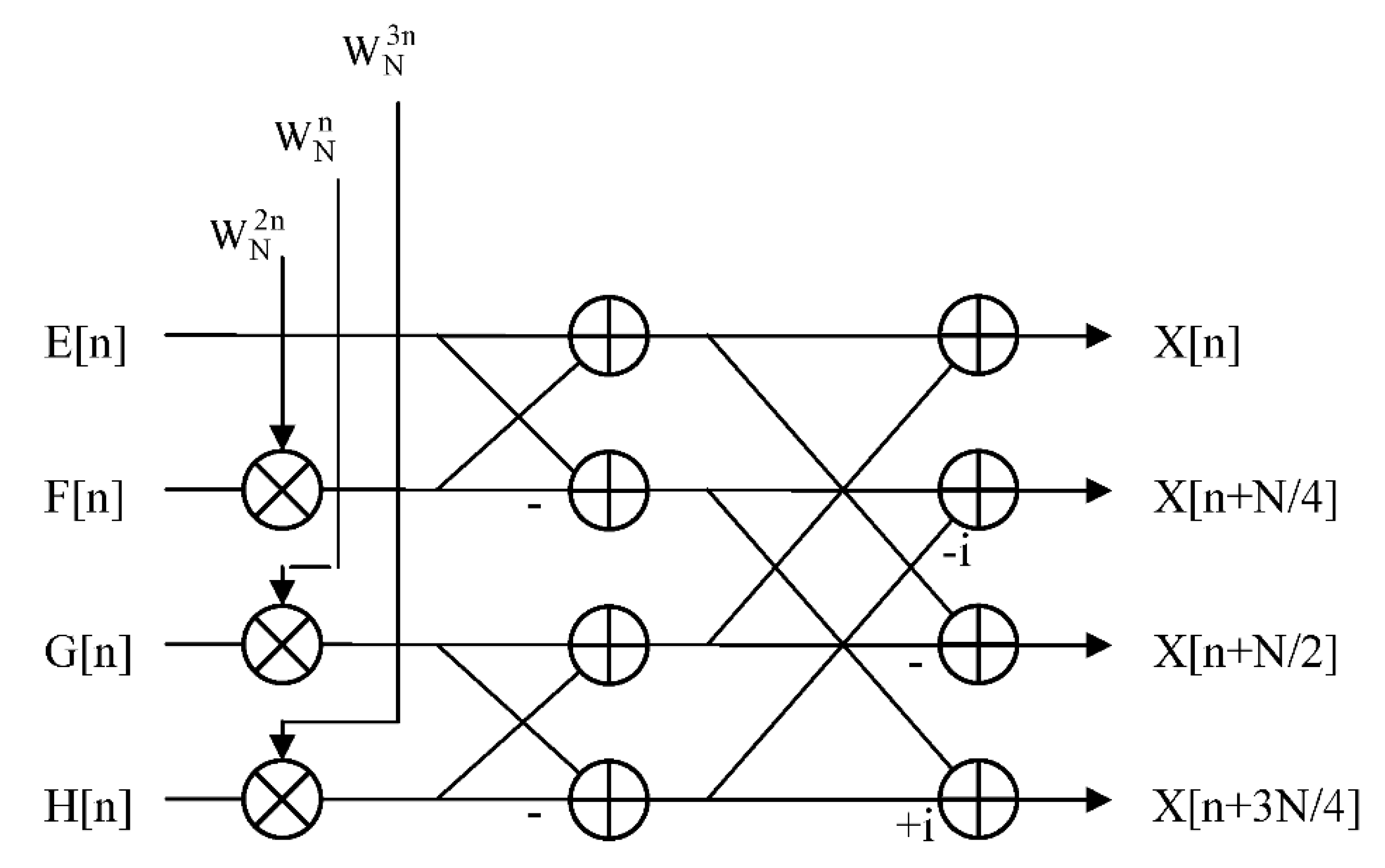
Figure 2.
Signal flow graph for DIFRN version of radix-4 FFT butterfly.
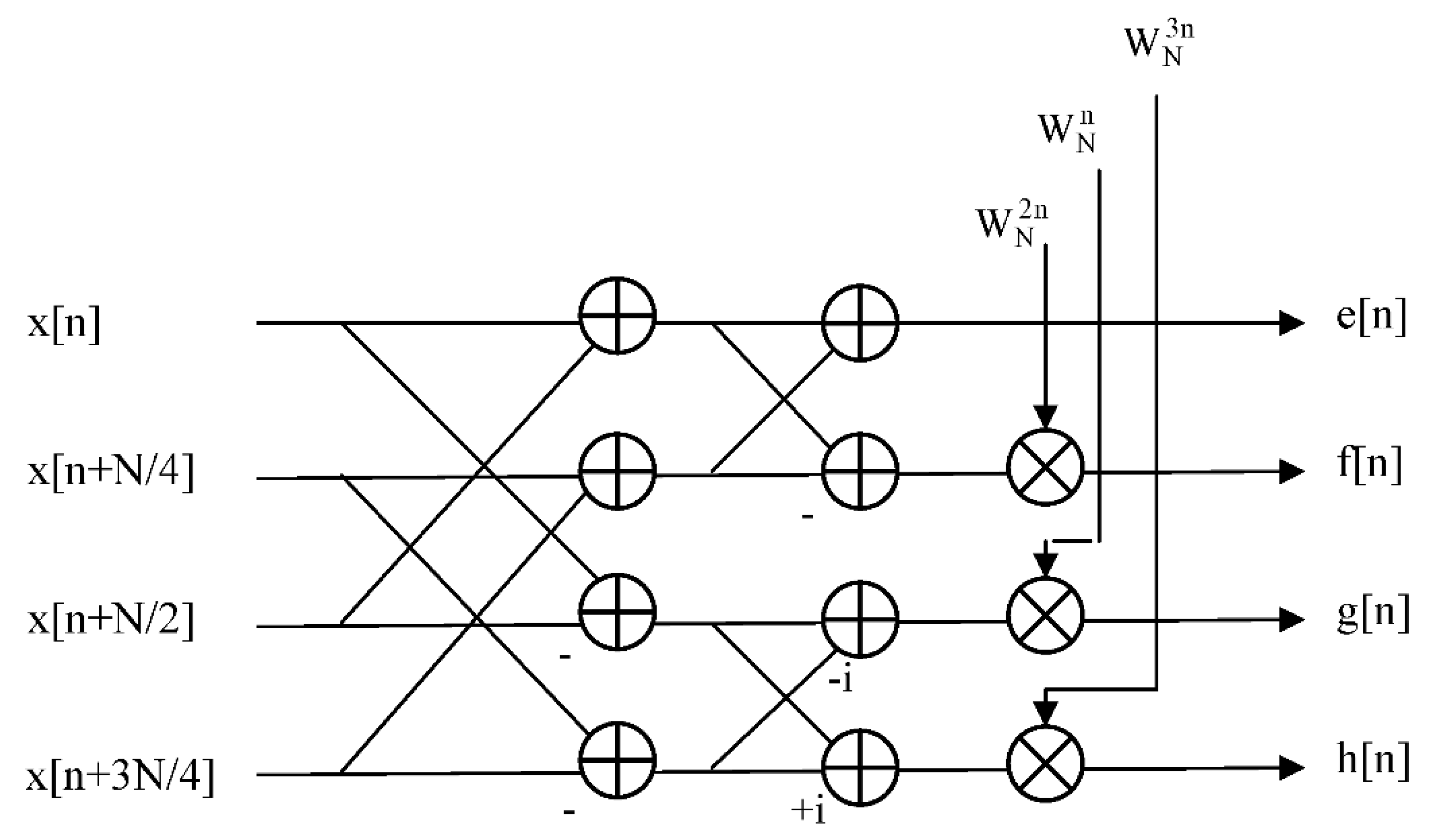
Figure 3.
decomposition of single quadrant of cosine function into coarse-resolution and fine-resolution angular regions using two single-level LUTs each of length 4.
Figure 3.
decomposition of single quadrant of cosine function into coarse-resolution and fine-resolution angular regions using two single-level LUTs each of length 4.
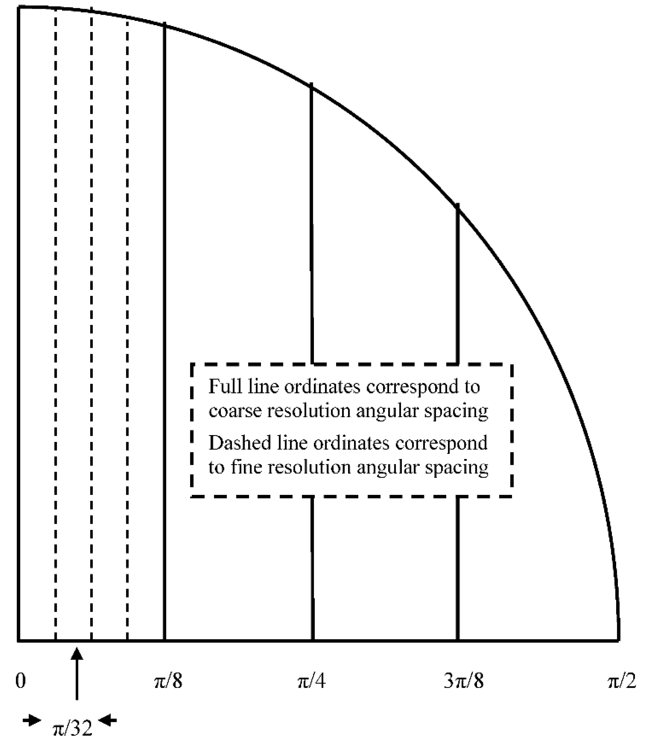
Figure 4.
Twiddle factor computation using two-level LUT with contents combined via standard two-angle identity.
Figure 4.
Twiddle factor computation using two-level LUT with contents combined via standard two-angle identity.
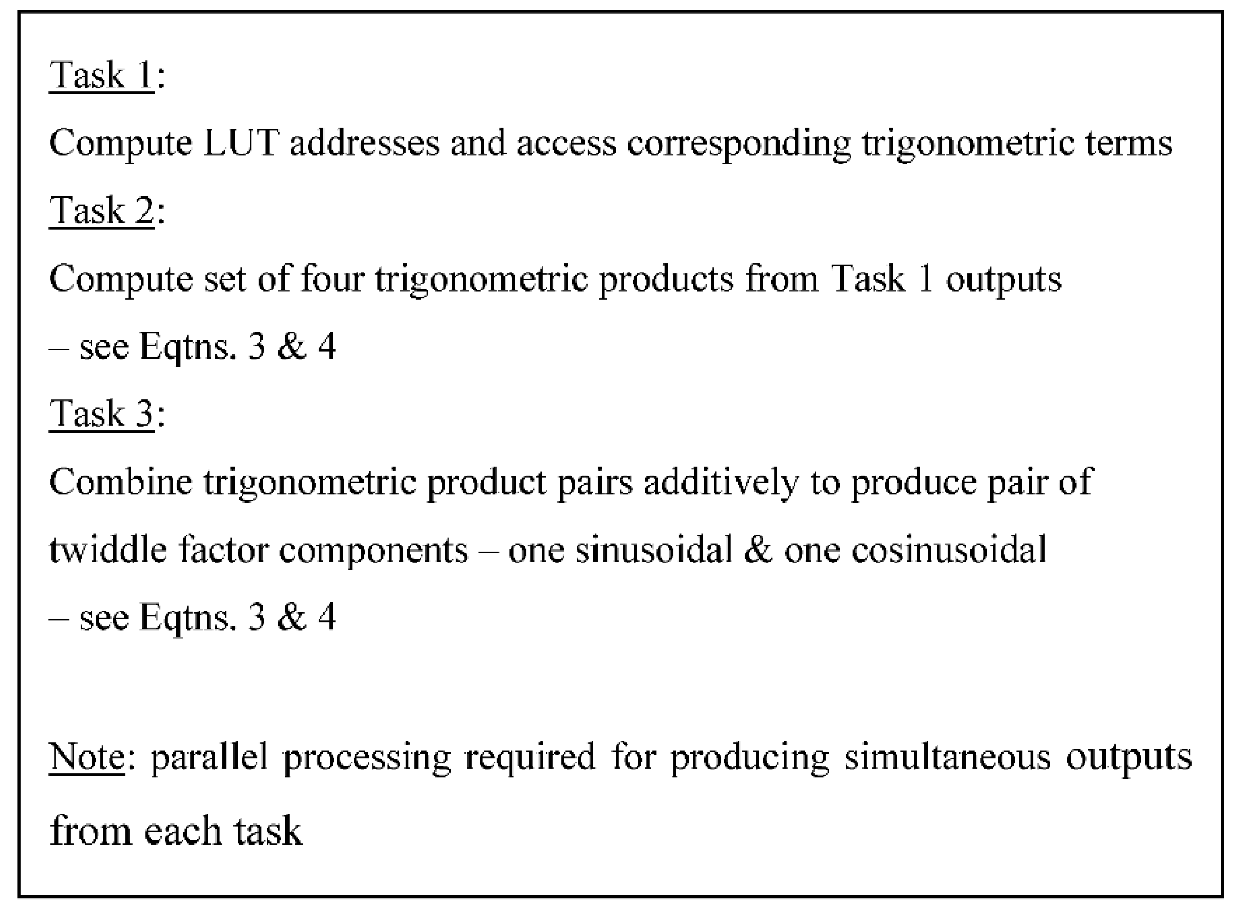
Figure 5.
SIMD computing architecture for solution to twiddle factor computation for radix-4 FFT butterfly.
Figure 5.
SIMD computing architecture for solution to twiddle factor computation for radix-4 FFT butterfly.
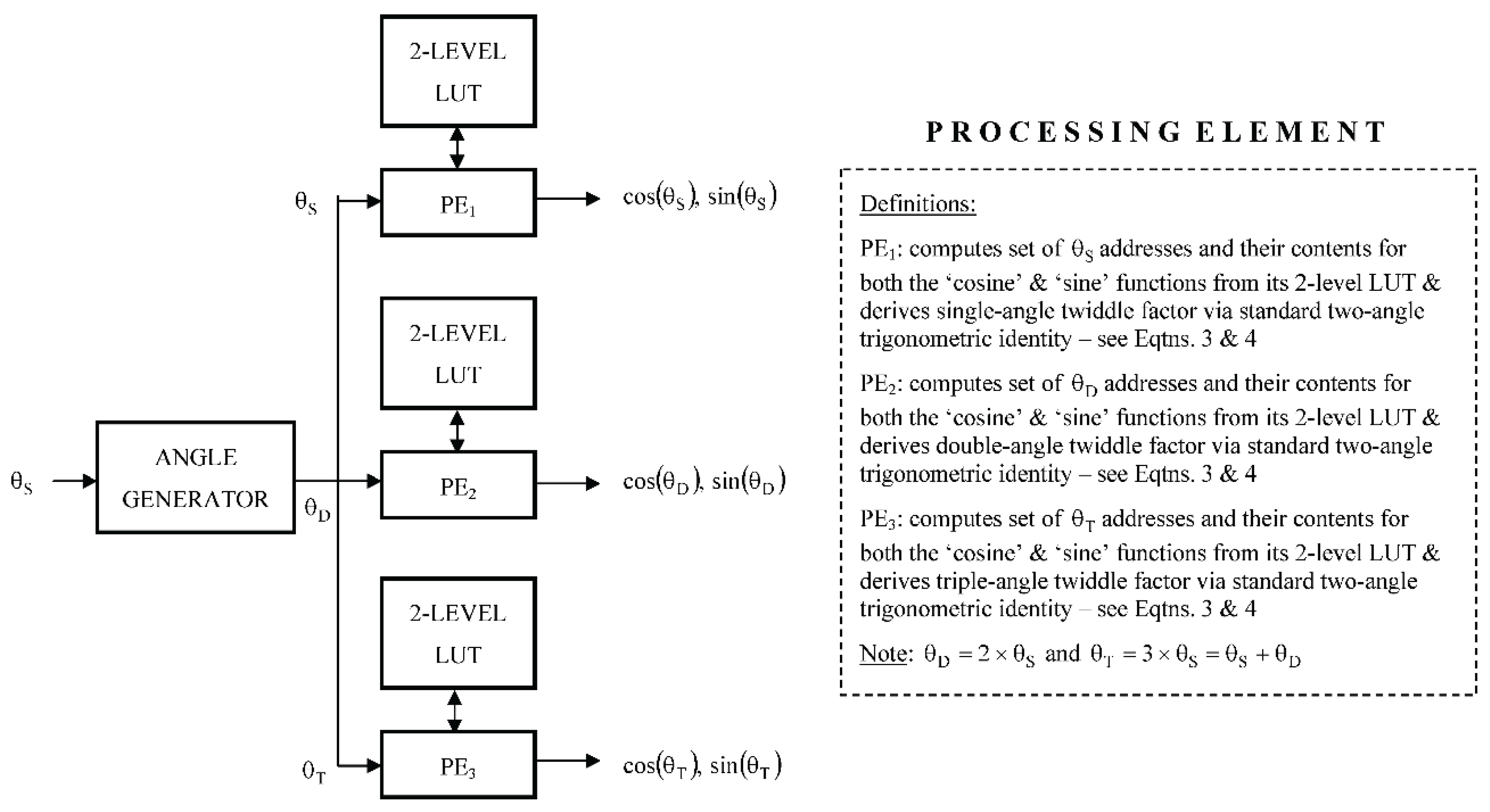
Figure 6.
pipelined computing architecture for solution to twiddle factor computation for radix-4 FFT butterfly.
Figure 6.
pipelined computing architecture for solution to twiddle factor computation for radix-4 FFT butterfly.
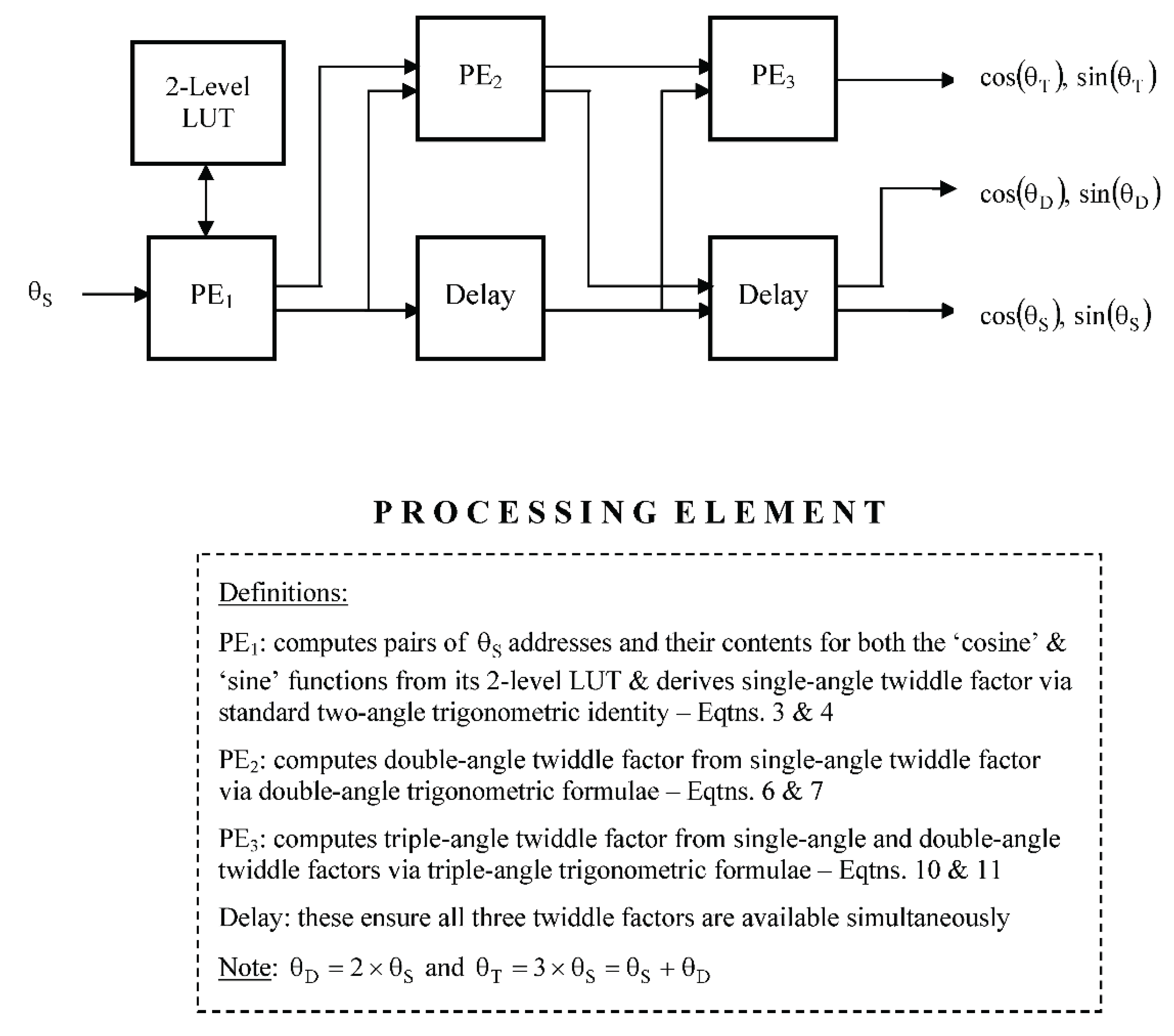

Table 1.
Arithmetic and memory requirements, per twiddle factor, for different LUT-based schemes.
| FFT Length | LUT-Based Scheme | Arithmetic Complexity | Memory Requirement (words) | Arithmetic + Memory Sizing (logic slices) | No Independent Tasks | |
| No Multiplications | No Additions | |||||
| 210 ~ 103 | 1-Level | 0 | 2 | 2.56×10² | ~ 6.14×10³ | 1 |
| 220 ~ 106 | 1-Level | 0 | 2 | ~ 2.62×10⁵ | ~ 6.29×10⁶ | 1 |
| 2-Level | 4 | 6 | ~ 1.54×10³ | ~ 2.58×10⁴ | 3 | |
| 230 ~ 109 | 1-Level | 0 | 2 | ~ 2.63×10⁸ | ~ 6.44×10⁹ | 1 |
| 3-Level | 8 | 10 | ~ 3.07×10³ | ~ 6.16×10⁴ | 5 | |
Note: word-length adopted for silicon sizing = 24 bits.
Table 2.
Space-complexity, per twiddle factor set, for different computing architectures.
| FFT Length | FFT Radix | Solution Type | Arithmetic Component | Memory Component (words) | |
| No Multipliers | No Adders | ||||
| 210 ~ 103 | 4 | SIMD | 12 | 18 | 1.44×10² |
| Pipeline | 8 | 9 | 0.48×10² | ||
| 8 | SIMD | 28 | 42 | 3.36×10² | |
| Pipeline | 24 | 17 | 0.48×10² | ||
| 16 | SIMD | 60 | 90 | 7.20×10² | |
| Pipeline | 56 | 33 | 0.48×10² | ||
| 220 ~ 106 | 4 | SIMD | 12 | 18 | ~ 0.46×10⁴ |
| Pipeline | 8 | 9 | ~ 0.15×10⁴ | ||
| 8 | SIMD | 28 | 42 | ~ 1.08×10⁴ | |
| Pipeline | 24 | 17 | ~ 0.15×10⁴ | ||
| 16 | SIMD | 60 | 90 | ~ 2.30×10⁴ | |
| Pipeline | 56 | 33 | ~ 0.15×10⁴ | ||
| 230 ~ 109 | 4 | SIMD | 12 | 18 | ~ 1.47×10⁵ |
| Pipeline | 8 | 9 | ~ 0.49×10⁵ | ||
| 8 | SIMD | 28 | 42 | ~ 3.44×10⁵ | |
| Pipeline | 24 | 17 | ~ 0.49×10⁵ | ||
| 16 | SIMD | 60 | 90 | ~ 7.37×10⁵ | |
| Pipeline | 56 | 33 | ~ 0.49×10⁵ | ||
Disclaimer/Publisher’s Note: The statements, opinions and data contained in all publications are solely those of the individual author(s) and contributor(s) and not of MDPI and/or the editor(s). MDPI and/or the editor(s) disclaim responsibility for any injury to people or property resulting from any ideas, methods, instructions or products referred to in the content. |
© 2025 by the authors. Licensee MDPI, Basel, Switzerland. This article is an open access article distributed under the terms and conditions of the Creative Commons Attribution (CC BY) license (http://creativecommons.org/licenses/by/4.0/).
Copyright: This open access article is published under a Creative Commons CC BY 4.0 license, which permit the free download, distribution, and reuse, provided that the author and preprint are cited in any reuse.


