Submitted:
13 May 2025
Posted:
14 May 2025
You are already at the latest version
Abstract
Land managers across the United States (U.S.) are developing plans to mitigate climate change. Effective implementation and monitoring of these climate action plans require standardized methods and timely, accurate geospatial data at appropriate resolutions. Despite the abundance of geospatial and statistical data in the U.S., a significant gap remains in translating these data into actionable insights. To address this gap, we developed the Land Emissions and Removals Navigator (LEARN), an online tool that automates subnational greenhouse gas (GHG) inventories of forests and trees in nonforest lands using a standardized analytical framework consistent with national and international guidelines. LEARN integrates multiple datasets to calculate land cover and tree canopy changes, delineate areas of forest disturbance, and estimate carbon emissions and removals. To demonstrate the application of LEARN, this paper presents case studies in Jefferson County, Washington; Montgomery County, Maryland; and federally owned forests across the conterminous U.S. Our results highlight LEARN’s capacity to provide localized insights into carbon dynamics, enabling subnational entities to develop tailored climate strategies. By enhancing accessibility to standardized data, LEARN empowers community land managers to more effectively mitigate climate change. Future developments aim to expand LEARN’s scope to cover nonforest landscapes and incorporate additional decision-making functionalities.
Keywords:
land use
; carbon
; forests
; trees outside forests
; climate change mitigation
; climate action planning
; local
1. Introduction
The land sector plays a pivotal role in global greenhouse gas (GHG) mitigation efforts. In 2022, the Land Use, Land-Use Change, and Forestry (LULUCF) sector in the United States (U.S.) had a net increase in carbon stocks of 921.8 million megagrams of carbon dioxide equivalent (million Mg CO2 eq.), effectively offsetting 14.5% of the nation’s total GHG emissions [1]. While forests play an outsized role in sequestering carbon from the atmosphere, they also cause significant emissions of greenhouse gasses when disturbed, burned or converted to nonforest land use. Trees on nonforest lands also absorb atmospheric carbon dioxide, while providing other ecosystem services, such as reducing urban heat [2] and regulating hydrologic systems [3].
While national GHG inventories offer valuable insights for guiding land management priorities, there is an increasing need for subnational and local GHG data to inform resource management and climate mitigation plans. Subnational entities, including state and local governments as well as private institutions, are instrumental in implementing land-use policies and practices that directly impact carbon emissions and sequestration [4].
However, lack of access to detailed, localized data hinders their ability to make informed decisions tailored to regional conditions. The U.S. Department of Agriculture (USDA) Forest Service (FS) Forest Inventory and Analysis (FIA) Program maintains one of the world’s most robust and comprehensive national forest inventory databases. Despite the wealth of data available, FIA data are often underutilized due to their complexity, scale, and lack of corresponding and accessible geospatial information. While some researchers are producing spatial datasets derived from FIA plot information [5], these datasets are challenging to apply to GHG inventories at local scales without specialized expertise.
Thus, there is a pressing need for standardized geospatial and statistical data that are timely, accurate, consistent and with sufficient resolution across jurisdictions and scales. Such standardized data can enable monitoring and reporting and facilitate collaboration among different stakeholders. Furthermore, keeping stock of carbon emissions and removals separately rather than combining them to track only the net GHG flux, can elucidate key drivers of change and highlight specific areas of improvement [6,7,8].
The Land Emissions and Removals Navigator (LEARN) is a free online tool and open-source codebase that performs automated GHG inventories of forests and trees at any scale within the conterminous U.S. from 2001 to 2023. LEARN is fully operational for use across the conterminous United States, with typical applications demonstrated through the case studies presented here (see Discussion for detailed considerations on appropriate scale and application). Built upon land use, forest inventory, and disturbance data from U.S. Department of Agriculture USDA FS, the U.S. Geological Survey (USGS), and other federal agencies, LEARN provides a user-friendly platform for generating localized GHG inventories using nationally consistent data and a standardized approach consistent with USDA and International Panel on Climate Change (IPCC) guidelines [9,10].
This paper builds upon the extensive peer-reviewed methodology with an emphasis on the multiple spatial and statistical data sources underpinning LEARN and presents case studies as examples that illustrate its applications in various contexts. By increasing accessibility to standardized geospatial data and statistical analysis, LEARN aims to empower subnational entities and communities to participate more effectively in climate mitigation planning and implementation.
2. Methods
2.1. Conceptual Framework
LEARN’s conceptual framework applies standard USDA and international analytical methods designed to be fit-for-purpose for communities while preserving the detail necessary to provide useful data for informing local climate change mitigation policies. Methods applied in LEARN were reviewed and published originally as an appendix to the ICLEI – Local Governments for Sustainability (ICLEI) U.S. Community Protocol [11] and subsequently expanded for international applicability through the publication of a standalone supplement to the Greenhouse Gas Protocol’s Global Protocol for Community-Scale Greenhouse Gas Inventories [12].
The methods are also aligned with the 2024 update to USDA’s entity-scale GHG inventory guidelines [9]. A technical note [13] documented the data inputs, methods, and processes behind version 1.1 of the LEARN tool. That document, though not peer-reviewed in a journal context, underwent extensive internal and external stakeholder review and is referenced here for transparency, reproducibility, and ease of access to methodological details not fully captured within the constraints of this manuscript.
All guidance documents upon which LEARN is based have been extensively reviewed by experts and follow the IPCC Guidelines for National Greenhouse Gas Inventories [10] both in the equations used and in the way land-related GHGs are conceptualized. Of the two equally valid methods offered in the IPCC Guidelines for estimating net C fluxes from land (stock-change and gain-loss), LEARN applies the gain-loss approach. The gain-loss method was chosen for LEARN because few communities have sufficient plot data available to use the stock-change approach. Furthermore, the gain-loss approach allows for the estimation of emissions and removals separately, which is helpful for designing policy interventions. While the term “removals” in forest inventories can sometimes refer to activities like timber harvesting, in this paper “removals” specifically refers to the process by which trees and plants absorb carbon dioxide from the atmosphere and store it as carbon in biomass and soils—a process also known as carbon sequestration.
The approach summarized below represents an application of the “gain-loss” method described by IPCC and often used in national GHG inventories. Land use and land use changes have associated emissions (GHGs lost from lands) and removals (carbon accumulated into ecosystem vegetation and soils). Both emissions and removals are represented by activity data multiplied by emission factors: represented by activity data multiplied by emission factors:
where:
Where activity data (AD) describes an area of categorized land use or land-use change and emission factors (EF) or removal factors (RF) describe the annual change in Ce per area unit. The complete description of the IPCC gain-loss method is presented in the annex to Appendix J [11]. The methods described here directly support IPCC Tier 2 and Tier 3 approaches, as detailed in Appendix B.1.
2.2. Data Sources and Applications
LEARN integrates a range of spatial and tabular datasets to perform inventory analyses, summarized in Table 1 according to their specific applications: land cover change detection, disturbance identification, and derivation of emission and removal factors. LEARN primarily utilizes datasets at a 30-meter resolution, making it most suitable for subnational analyses such as counties, municipalities, and regional landscapes. Although technically possible, applying LEARN at significantly finer (e.g., parcel-level) or broader scales (e.g., multi-state regions) may introduce uncertainties related to dataset resolution limitations and aggregation effects (see Section 4.3 for further details).
Most datasets integrated within LEARN are national in scope and applicable to subnational analyses across the conterminous U.S. A global dataset [14] is specifically used to delineate harvest because no comparable national dataset is available at suitable resolution to capture harvest disturbances comprehensively on both public and private lands. These datasets are integrated using a Python-based geospatial modeling framework to quantify land cover and tree canopy changes, identify forest disturbances, and derive accurate carbon emission and removal factors. The methods outlined below summarize the general approach for generating and integrating activity data and carbon factors. Detailed geoprocessing steps and code documentation are publicly available in the accompanying GitHub repository (see Data Availability Statement).

Table 1.
Data sources for calculation of GHG inventories in LEARN. For more detailed descriptions, see Glen et al., 2024 [13]
Table 1.
Data sources for calculation of GHG inventories in LEARN. For more detailed descriptions, see Glen et al., 2024 [13]
| Variable | Dataset | Source | Resolution | Years Available in Tool |
|---|---|---|---|---|
| Land Cover | ||||
| Land Cover | National Land Cover Database (NLCD) | [15] | 30 meters | 2001, 2004, 2006, 2008, 2011, 2013, 2016, 2019, 2021, 2023 |
| Tree Canopy | ||||
| Tree Canopy Cover | National Land Cover Database (NLCD) | [15] | 30 meters | 2011, 2013, 2016, 2019, 2021, 2023 |
| Forest Disturbances | ||||
| Forest Fires | Monitoring Trends in Burn Severity (MTBS) | [16] | 30 meters | 2001–2023 (annual) |
| Insect and Disease | Insect and Disease Detection Survey | [17] | Varies | 2001–2023 (annual) |
| Timber Harvest and Other | Global Forest Watch Tree Cover Loss | [14] | 30 meters | 2001–2023 (annual) |
| Estimating Emission and Removal Factors | ||||
| Removal Factors | ||||
| Forest Type | FIA Forest Type Groups | [5] | 30 meters | Single estimate for 2014–2018 |
| Plantations | Spatial Database of Planted Trees (v1) | [18] | Varies | 2015 |
| Forest Age | FIA Forest Stand Age | [5] | 30 meters | Single estimate for 2014–2018 |
| Undisturbed Forests | FIA Database | [19] | Non-spatial | Varies by region and variable combinations |
| Afforestation or Reforestation | FIA Database | [19] | Non-spatial | Varies by region and variable combinations |
| Trees outside forests | Urban Trees Emission and Removal Factors | [20] | Non-spatial | 2005 |
| Emission Factors | ||||
| Carbon Stocks | BIGMAP Forest Carbon Pools | [5] | 30 meters | Single estimate for 2014–2018 |
| Trees outside forests | Urban Trees Emission and Removal Factors | [20] | Non-spatial | 2005 |
| Forest Disturbances | Regionally modeled disturbance database | [21] | Non-spatial | Derived from FIA data (2001–2010) |
2.3. Activity Data Generation
Detailed methodological steps for generating activity data are provided in Appendix A. This section provides a condensed overview.
2.3.1. Land Cover and Land Use
The terms land use and land cover are often used interchangeably but have important distinctions relevant to emissions accounting. Land use refers to the management and intended purpose of land (e.g., cropland, forest land), whereas land cover describes physical vegetation or surface characteristics (e.g., grassland, shrubland, forest cover). LEARN integrates satellite-derived land-cover data (primarily from NLCD) and explicitly includes additional disturbance datasets (such as fire and insect/disease maps), which improve differentiation between temporary disturbances and permanent land-use transitions by providing specific spatial and temporal context for disturbance events. Nonetheless, this integrated approach still has limitations, as land-cover maps alone may not fully distinguish temporary changes (e.g., fire or harvest) from permanent conversions (e.g., urban development or agricultural expansion). Therefore, additional contextual analysis and integration of local knowledge or ground-based data are recommended to further refine LEARN’s categorization of emissions and removals (see Section 4).
2.3.2. Land Use Change Matrices
Activity data are calculated using a land use change matrix approach [10], in which spatially and temporally explicit data derived from 30-meter Landsat satellite imagery are used to track individual pixels consistently through time. NLCD is specifically designed to be harmonized over time so that classification changes in a pixel over a time series are more likely to represent actual changes on the ground. In this approach, area (ha) of total losses and gains in specific land-use categories can be calculated, as well as what these conversions represent. The NLCD datasets for start year and end year of an inventory period are combined to create a land cover change matrix. The detailed land cover change values are recategorized (see Figure A1) to the into six standard IPCC land-use categories (Forest Land, Cropland, Grassland, Settlements, Wetlands and Other Land) to create a simplified transition matrix (see Figure 1). Transitions identified in the NLCD data are aggregated into four key categories (Forests Remaining Forests, Forest to Nonforest, Nonforest to Forest, Nonforest Remaining Nonforest) based on IPCC standards, which directly inform subsequent emission and removal calculations (see Figure 2). The Forests Remaining Forests and Nonforest Remaining Nonforest categories are further stratified as described in Section 2.3.3 and Section 2.3.4 below.
2.3.3. Forests Remaining Forests
Areas of forest land remaining forest are further stratified as either undisturbed or disturbed (Figure 2), depending on their overlap with disturbance datasets during the inventory period. For each inventory period, spatial information about the location and timing of disturbances are estimated using a hierarchical combination of fire [16], insect and disease mortality [17], and tree cover loss ([14], updated annually on Global Forest Watch). Any areas of tree cover loss during the inventory period that do not overlap with fire or insect and disease mortality are assigned to the “harvest or other” category. This methodology aligns with findings from [22], who determined that from 1986 to 2010, less than 1% of forest disturbances in the United States could be attributed to causes outside of fire, insect/disease ("stress"), or harvest.
Low-severity disturbances, defined as those resulting in less than 50% canopy loss, are excluded from explicit disturbance classifications due to their typically rapid recovery, as corroborated by [21]. These disturbances are thus implicitly considered within the undisturbed forest category, as they do not substantially alter long-term forest carbon dynamics within the inventory timeframe. Disturbances in areas outside of forests remaining forests (e.g., fire in grasslands) are excluded.
2.3.4. Nonforest Remaining Nonforest
In any nonforest areas that remained nonforest during the inventory period, emissions and/or removals from changes from one land use class to another (e.g. grassland to cropland) are not calculated individually. Rather, in this category LEARN estimates emissions and removals from NLCD Tree Canopy Cover change over the inventory period. Where tree canopy data do not exactly align with NLCD land cover data periods, canopy metrics are annualized by averaging available overlapping data points to estimate consistent annual change rates for the inventory period. Within areas that remained nonforest over the inventory period selected, tree canopy data for start and end year of the inventory period are compared to derive gross tree canopy loss. Tree canopy maintained or gained is estimated by averaging the total tree canopy cover areas in the start and end years of the inventory period.
2.4. Deriving Emission and Removal Factors
This section provides a condensed overview of underlying assumptions and methods for deriving emission and removal factors. A thorough description with detail is provided in Appendix B. A complete list of emission and removal factors is provided in Supplementary Materials Table S.1.
2.4.1. Forests Remaining Forests
Undisturbed Forests. Removal factors for undisturbed forests are generated using the FIA database via EVALIDator [23]. Data stratification includes management regions from [24], FIA forest-type groups, stand origin, and age class distributions. Plots with recent disturbances or atypical stocking levels are excluded. Detailed methodology for the development of removal factors in undisturbed forests is provided in Appendix B.4. A complete list of removal factors for undisturbed forests by region, forest type, age class, and origin are provided in Supplementary Materials Table S.1.
Disturbed Forests. Emission factors for forest disturbances within the inventory area are calculated by mapping unique combinations of forest region, forest type group, disturbance type, and disturbance severity to a database of emission factors developed by the USDA FS and collaborators [25] based on methods reported in [21]. Additional methodological considerations are documented in Appendix B.8. Detailed emission factors are available in Supplementary Materials Table S.1.
2.4.2. Forests and Land Use Change
Forest Converted to Nonforest. For any pixel delineated as forest converted to nonforest land uses, a carbon stock value for the forest is calculated for three aggregated carbon pools: living biomass (aboveground, belowground, and understory), dead organic matter (standing dead, down dead, and litter), and organic soil carbon [5]. Emissions are estimated by applying default national carbon loss percentages provided by the [26] to mapped values for pre-conversion biomass, dead organic matter, and soil carbon pools (Table A4). Calculations and assumptions are further described in Appendix B.7.
Nonforest Converted to Forest. Areas of new forest establishment via reforestation or afforestation are assigned removal factors based on forest region and forest type group. Removal factors were developed by querying FIA data using the same methods for the 0–20-year age class of undisturbed forests, with additional adjustments for soil organic carbon accumulation during early forest establishment (following [27]). Additional information is provided in Appendix B.5. The complete table of removal factors for nonforest converted to forest is available in Supplementary Materials Table S.1.
Nonforest Remaining Nonforest. Emission and removal factors for trees outside forests are derived from [20]. Emission factors associated with canopy loss are determined at the city level, based on direct measurements and detailed urban canopy assessments from representative cities within each state or region. These representative cities were selected based on data availability, urban tree composition similarity, and geographic representativeness. Removal factors related to canopy maintained or gained during an inventory period utilize state-level averages due to limited availability of detailed local measurements for canopy growth across all communities. Additional methodological details including selection criteria for representative cities are provided in Appendix B.6. Complete factor tables are included as Supplementary Materials (Table S.2)
2.5. Case Studies
LEARN analyses were conducted for three specific areas of interest over four periods: 2013-2016, 2016-2019, 2019-2021 and 2021-2023.
2.5.1. Community Inventories
Two of the analyses are community GHG inventories, selected to demonstrate diversity in community land bases and data applications. Jefferson County, Washington is a large (5,650 km2), sparsely populated county with significant forested area including Olympic National Park and National Forest. Montgomery County, Maryland is a smaller (1,310 km2) but more populated county [28], with a range of settlement densities, patchworks of cropland and pasture, and deciduous forests. Spatial boundaries for both counties were extracted from the US Census TIGER/Line dataset [28].
The community GHG inventories include analyses of forests and trees outside forests (tree canopy extent, tree canopy loss) and associated carbon sequestration and emissions. For trees outside forests, emission and removal factors were selected based on proximity to representative cities and states. Specifically, for Montgomery County, the emission factor from Baltimore, Maryland, and the removal factor for the state of Maryland were applied. Similarly, for Jefferson County, Washington, the emission factor from Seattle, Washington, and the removal factor from the state of Washington were used (see Supplementary Materials Table 2 for a complete list of emission and removal factors applied to trees outside forests). Because the 2023 NLCD Tree Canopy data were not yet available at the time of publication, tree canopy data from 2019 to 2021 were used for the 2019–2023 inventory period.
2.5.2. Federally Owned Forests
The third case study focuses on forests remaining forests (see 2.3.2) in federally owned forest lands across the CONUS. The PAD-US database [29] was used to delineate forest ownership. The database was filtered to ownership by USDA FS or the Bureau of Land Management (BLM), then dissolved by state to correct overlapping or broken geometries. Because this case study is focused on forests remaining forests and excludes trees outside forests, tree canopy data was not included in the analysis.
2.6. Validation Exercise
To validate our results, we performed independent queries of the U.S. Forest Inventory and Analysis (FIA) database for each of the case study areas using the EVALIDator query system [23], and compared the FIA stock-change estimates with the LEARN “net flux” estimates, which should be of similar magnitude for forests by excluding estimates for trees outside forests from LEARN since these are not included in the FIA database. The inventory periods, however, are not fully comparable due to differences in remeasurement intervals. FIA remeasurement cycles typically range from 5 to 10 years depending on the region, generally shorter in the eastern United States and longer in the West, while LEARN inventory periods are user-defined and can vary widely but often span intervals aligned with National Land Cover Database (NLCD) releases, typically 2 to 3 years apart. Therefore, some temporal mismatch between FIA remeasurements and LEARN estimates should be considered when interpreting validation results. For community inventories, comparisons between LEARN and FIA included forests remaining forests and forest change, but excluded trees outside forests. For federally owned forests, comparisons included forests remaining forests only.
3. Results
3.1. Community Inventories
3.1.1. Jefferson County
Jefferson County had significant net GHG removals by forests and trees in all four inventory periods (see Figure 3 and Table 2). The magnitude of net removals averaged about -3.89 million Mg C/year from 2013-2023, roughly equivalent to the emissions from driving 900,000 gasoline-powered passenger vehicles for one year [1]. The net sink decreased about 24% from 2013-2016 to 2019-2023, driven by an increase in emissions from forest conversion and disturbances.
Gross removals are approximately -5.03 million Mg C/year, on average, and average gross emissions roughly 1.13 million Mg C/year. Most of the carbon removals in the Jefferson County Inventory (95%) came from undisturbed forests. Forests disturbed by insects and disease, while sequestering less carbon than an undisturbed forest, remove an average of roughly -142.7 thousand Mg C/year. Nonforest to forest change accounts for roughly 2% of gross removals. Trees outside forests contribute about 3% of gross removals.
The largest cumulative sources of emissions are forest to grassland changes and disturbances in the harvest/other category, comprising an average of 52% and 41% of gross emissions, respectively. Emissions from forest-to-grassland changes and harvest disturbances were spatially clustered, predominantly in areas identified as private or state forest lands. Areas identified as forest to grassland change occur in larger blocks compared to a more dispersed pattern in areas identified as disturbed by harvest/other. (Figure 4).
A validation exercise comparing LEARN and FIA estimates showed that LEARN estimated similar net C flux for Jefferson County as FIA estimates (-3.88 million Mg C/year during 2019-2021 compared to FIA’s -3.97 million Mg C/year during a similar period, respectively, excluding trees outside forests). The forest area estimated by LEARN was nearly identical to FIA, about 2% greater. (Table 5).
3.1.2. Montgomery County
Montgomery County’s gross emissions decreased steadily over the four inventory periods from 2013 to 2023, showing a reduction of 39% from the first inventory to the last (See Figure 5 and Table 3). This reduction was due largely due to decreasing emissions from nonforest tree canopy loss which contributed 94% of cumulative gross emissions on average. Most of this nonforest tree canopy loss in Montgomery County from 2013-2023 occurred in settlement land use areas (81%). Other emission sources such as forest conversion and forest disturbances accounted for only about 6% of gross emissions, with the harvest/other disturbance category as the largest forest emissions source.
Montgomery County maintained an average net carbon sink of roughly -429.7 thousand Mg C/year from 2013-2023, with notable variation across inventory periods. The net sink increased by approximately 20% from 2013–2016 to 2019–2021, driven primarily by decreased emissions from tree canopy loss. However, there was a 6% uptick in tree canopy loss area and associated emissions between the 2019–2021 and 2021–2023 periods. Gross removals were roughly 55% from nonforest tree canopy and 45% from undisturbed forests.
LEARN estimated the net flux of C for Montgomery County forests at less than half compared with an independent FIA query (-242.3 thousand Mg C/year vs. FIA’s -629.4 thousand Mg C/year, excluding trees outside forests). The area of forest land was similar for both estimates, with minimal influence from disturbances or harvesting.(Table 5). Possible reasons for these differences are explored in Section 4.1.
Patches of tree canopy loss (see Figure 6) are widespread across Montgomery County and occur primarily in urban land use areas. The pattern of tree canopy loss is decentralized in many small patches as opposed to large blocks of loss.
3.2. Federally Owned Forests
The net carbon sink from federally owned forests was roughly -133.91 million Mg C/year from 2013 to 2023, with a decrease in net removals in the 2019–2021 period (Figure 7, Table 4). Gross removals remained relatively stable at an average of -175.17 million Mg C/year. The observed decrease in net removals was driven primarily by increased emissions from fire disturbances, which increased by more than 400% from the 2013–2016 period to the 2019–2021 period. Emissions from the harvest/other category also increased from 2013-2023, with annual average emissions rising about 65% from the 2013-2016 to 2021-2023 periods. In some cases, disturbances from insect/disease can result in overall net emissions (2013-2016 period), while in other cases they can result in overall net removals (2016-2019 period), though these are always reported within the emissions category in the inventory.
Land ownership and forest disturbances have high spatial heterogeneity across CONUS. Figure 8.a provides an overview of federal land ownership, which is highly concentrated in the Western States. Figure Figure 8.b shows forests remaining forests within federally owned lands in Western Colorado, where disturbance from fire and insect/disease is prevalent. LEARN estimated the net flux of C for federally owned forests at approximately -133.91 million Mg C/year, similar to the FIA’s independent estimate of -129.01 million Mg C/year. Forest area differed significantly between estimates: LEARN estimated around 49.80 million hectares versus FIA’s 67.61 million hectares. Both estimates indicated significant emissions from fire and harvesting, though direct comparisons are complicated by differences in inventory periods and the resolution of small-scale disturbances (Table 5).
4. Discussion
The LEARN tool provides a robust approach to developing subnational GHG inventories by integrating publicly available spatial datasets with ground-sourced forest and tree inventory data. This standardized yet flexible framework bridges a critical gap between national-level aggregation and local-level action, enabling jurisdictions to effectively monitor changes in carbon sources and sinks from forests and trees and to inform climate strategies at a local level. Case studies from Jefferson County, Montgomery County, and federally owned forests demonstrate the practical utility and adaptability of LEARN across varying scales and land-management contexts.
4.1. Interpretation of Case Studies
The case studies of Jefferson and Montgomery counties illustrate LEARN’s practical applications and implications for local climate strategies. In Jefferson County, the significant average net sink of approximately -3.89 million Mg C/year highlights the critical role that forests and trees play in regional climate mitigation strategies. However, substantial temporal variation in emissions from forest disturbances and land-use changes emphasizes the importance of understanding and managing local drivers of emissions.
A significant portion of emissions in the Jefferson County inventory (52%) were found to be from forest to grassland changes. Challenges exist in differentiating between emissions resulting from land use and land cover changes, especially for forests. Major forest disturbances such as fires may be classified as land cover changes transitions from forest to grassland. Conversely, areas designated as grassland might inaccurately appear as forest transitions during early recovery phases after disturbances. Thus, clearly distinguishing temporary disturbances from permanent changes is vital. Jurisdictions like Jefferson County finding large changes between forest and grassland should conduct supplemental analyses to correctly identify and categorize emissions and removals.
Notably, FIA retrievals for Jefferson County yielded similar results for both forest area (390.7 thousand ha for LEARN and 384.5 thousand ha for FIA) and net flux (-3.88 million Mg C for LEARN and -3.97 million Mg C for FIA). However, careful interpretation is advised regarding this alignment, particularly given the fundamental methodological differences between LEARN and FIA. LEARN primarily uses remotely sensed spatial data combined with FIA emission and removal factors to estimate carbon fluxes, which provides broad geographic coverage but may overlook fine-scale variability. In contrast, FIA utilizes detailed ground-based plot measurements, offering higher precision but potentially missing broader landscape-level dynamics. Also, temporal mismatches affect results, with remote sensing observations being more aligned with specific dates of data collection compared with FIA that spans longer and older inventory periods. These methodological distinctions inherently limit direct comparability and may contribute to discrepancies observed in other case studies, such as Montgomery County and federally owned forests. Therefore, while the Jefferson County results suggest promising consistency, users should recognize these methodological constraints and pursue supplemental validation to ensure accurate and context-specific interpretation for local climate strategies.
Montgomery County illustrates distinct challenges given its smaller forested area and higher development density. The steady decrease in emissions from tree canopy loss within settlement areas could suggest effective local management practices. However, recent slight upticks in emissions indicate the need for continued vigilance and monitoring to sustain progress. LEARN estimated the net flux of C for Montgomery County at less than half compared with an independent FIA query, excluding trees outside forests. The area of forest land was similar for both estimates, with neither showing significant influence from disturbances or harvest. The difference is likely due to other factors, such as different dates of inventory data, regional removal factors potentially set too low given Montgomery County’s position at ecological boundaries between the Northeast and Southeast regions, and uncertainties inherent in estimating fluxes for relatively small, forested areas. Users encountering similar discrepancies should carefully review and consider revising local removal factors to enhance accuracy.
Federally owned forests provide insights into broader-scale dynamics affecting carbon sinks, notably highlighting significant increases in emissions from fire disturbances and timber harvesting activities. LEARN estimated the net flux of C for federally owned forests similarly to an independent FIA query (-133.90 million Mg C/year vs. FIA’s -129 million Mg C/year). However, significant differences in estimated forest area exist: LEARN estimated approximately 49.80 million hectares compared to FIA’s 67.6 million hectares. These discrepancies are primarily because NLCD data classifies some areas without trees as non-forest land, while FIA classifies these areas based on land use as forests. Since these areas lack substantial tree cover, this discrepancy in forest area has limited influence on the net C flux. Both estimates indicate significant emissions from fire and harvesting activities, though direct comparisons are challenging due to differences in inventory periods and LEARN’s limited representation of small-scale disturbances. These area discrepancies reinforce the need for explicit local verification and interpretation of results.
4.2. Methodological Considerations and Recommended Improvements
Despite LEARN’s strengths, several methodological considerations and uncertainties remain. First, LEARN currently assesses land-use changes involving only forests and trees outside forests and does not address other significant land-use types such as cropland and pasture. Expanding LEARN to include soil carbon stock changes in nonforest landscapes would significantly enhance its utility for jurisdictions with diverse land-use profiles. Within forest analyses, LEARN currently focuses exclusively on C due to the greater availability and standardization of spatially explicit datasets and emission/removal factors. However, we acknowledge the significant emissions of other greenhouse gases such as methane (CH) and nitrous oxide (NO), particularly from disturbances like fires or specific land-management practices. Future developments of LEARN aim to integrate these additional greenhouse gases once reliable, spatially explicit methodologies and datasets become broadly available.
Second, the geospatial data integration approach employed by LEARN provides a scalable and consistent methodology but introduces uncertainty. Although LEARN utilizes the latest publicly available datasets, these datasets vary in accuracy and often lack comprehensive uncertainty documentation. Additionally, uncertainties associated with scale and resolution affect the interpretation of LEARN’s outputs. Applying LEARN at scales finer than intended, such as individual parcels, may amplify data uncertainty due to limitations in dataset resolution. Conversely, aggregating data to broader scales can obscure local dynamics and introduce classification challenges. Establishing standardized methods for uncertainty documentation and reporting across LEARN’s components could increase user confidence and transparency.
Third, accurately delineating forest disturbances—especially timber harvests—remains challenging due to the lack of dedicated national datasets explicitly tracking harvest activities. LEARN applies a hierarchical rule to classify disturbances (fire > insect mortality > harvest or other disturbances), but events such as windthrow or weather-related disturbances can be mistakenly classified as harvests. Given that harvest, insect, and fire disturbances constitute most forest disturbances in the conterminous United States [22], LEARN relies on a process of elimination based on assumptions. Developing robust delineations of forest disturbances and improving the classification of temporary versus permanent land-use changes could reduce misclassification errors. Land managers with significant areas of harvest or other disturbances should evaluate contextual data to accurately identify disturbance causes and refine their policy decisions accordingly.
4.3. Implications and Guidance for Users
Considering the methodological challenges and uncertainties described above, users should verify automated outputs against local knowledge and supplemental data to distinguish temporary disturbances from permanent land-use changes. Contextual analyses are essential to accurately differentiate types of disturbances, particularly distinguishing harvests from other forms of forest disturbance. A particular challenge users should actively address is differentiating between temporary land-cover changes due to disturbances (e.g., forest harvests or fires) and genuine, permanent land-use transitions (e.g., permanent deforestation or urban development). Because LEARN relies on satellite-derived land-cover data (primarily NLCD) as proxies for land-use changes, misclassification can occur, especially in areas recently disturbed by forest harvests or stand-replacing events, where temporary grassland or shrubland cover might appear.
To mitigate potential misclassification, users are encouraged to incorporate supplemental analyses using aerial imagery, local forest-management records, or ground-based inventories. Such verification can confirm whether significant changes detected by LEARN represent temporary disturbances or actual land-use conversions. Additionally, users should consider cross-validating LEARN results with complementary datasets that explicitly classify land use, such as the FIA land-use classifications or emerging national land-use mapping products. Integrating these additional data sources can significantly refine the accuracy and reliability of GHG inventories generated by LEARN.
It is crucial that users align the spatial scale of their analyses with the resolution of input datasets to avoid magnifying inaccuracies or overlooking critical local details. Although LEARN is fully operational across the entire conterminous United States, its optimal application is at subnational scales—such as counties, municipalities, and regional landscapes. LEARN primarily uses datasets provided at a 30-meter resolution, effectively supporting analyses at these scales. While the tool can technically produce inventories at finer scales (e.g., parcel-level) or broader scales (e.g., multi-state regions), users should exercise caution with such applications. Finer-scale analyses can amplify uncertainties inherent in input datasets, while overly broad analyses might obscure critical local variations. Carefully matching analytical scale with data resolution ensures more meaningful and reliable results.
LEARN’s reliance on 30-meter resolution data from NLCD aligns well with recommendations from recent literature [30], which highlight that extremely high-resolution satellite-based forest carbon maps (0.3–5 m) may significantly increase uncertainty and be less reliable for carbon monitoring. Spatial resolutions exceeding typical tree crown diameters (approximately 10–20 m for temperate forests) are most appropriate, confirming LEARN’s resolution as suitable for accurately capturing forest carbon dynamics at typical plot scales used in carbon accounting.
When significant discrepancies occur between LEARN outputs and independent datasets, users should evaluate and recalibrate local emission and removal factors accordingly. Subnational entities—cities, counties, states, or tribal nations—should clearly define jurisdictional boundaries when establishing net-zero or net-negative targets, recognizing contributions from lands beyond direct management control, such as federally managed areas. Clear delineation of jurisdictions, distinguishing locally managed from federally managed lands, is crucial for effectively setting and achieving climate targets. Proactive collaboration with data producers and funders can help identify emerging data needs, refine methodologies, and enhance support for local climate policies and land-use management strategies. By proactively addressing these methodological and interpretative challenges, users can significantly improve the reliability, accuracy, and policy relevance of GHG inventories derived using LEARN.
5. Conclusion
The LEARN tool has been applied in multiple subnational contexts across the conterminous United States, including but not limited to the examples presented here, reflecting its broad utility in various land-use and climate mitigation initiatives. These diverse applications illustrate how land-based greenhouse gas inventories can inform strategies aimed at reducing emissions and enhancing carbon sequestration. LEARN’s alignment with USDA and IPCC guidelines, combined with its accessibility and standardized framework, supports jurisdictions seeking to incorporate land sector dynamics into their climate action planning, particularly those with limited technical resources. By identifying key factors influencing local carbon balances—such as forest management, tree planting, and canopy maintenance—LEARN provides information that can help guide effective land management decisions. Continued user engagement and iterative refinement based on practical feedback will be essential to address remaining methodological limitations and ensure the tool continues to effectively support climate mitigation efforts.
Supplementary Materials
The following supporting information can be downloaded at: https://www.mdpi.com/article/doi/s1, Table S1: Emission and Removal Factors for Forests Remaining Forests and Nonforest to Forest; Table S2: Emission and Removal Factors for Trees Outside Forests.
Author Contributions
Conceptualization, N.H. and R.B.; methodology, N.H. and R.B.; formal analysis, E.G.; data curation, E.G. and A.S.; writing—original draft preparation, E.G., N.H., and R.B.; writing—review and editing, A.S.; visualization, A.S.; supervision, N.H. and R.B. All authors have read and agreed to the published version of the manuscript.
Funding
Funding for LEARN has been provided by Doris Duke Foundation, the Climate and Land Use Alliance, Woodwell Climate Research Center, ICLEI-USA and the Bezos Earth Fund.
Data Availability Statement
The code used for this analysis is available at: https://github.com/erin-glen/learn_analysis. The free online LEARN tool is available at: https://icleiusa.org/LEARN/. All input datasets used in this analysis are publicly available, and sources have been provided in the paper. Any derivative data products used in LEARN, such as the combined disturbance rasters or forest characteristics rasters, are available upon request. Please contact Erin Glen (erin.glen@wri.org) for any inquiries.
Acknowledgments
We are pleased to acknowledge the many organizations and individuals who have contributed to this work. We extend our gratitude to ICLEI-USA for leading community engagement, organizing training cohorts, and hosting the LEARN Tool on their website. Susan Minnemeyer and the Chesapeake Conservancy have been instrumental in piloting the use of high-resolution tree canopy data and organizing communities in the Chesapeake Bay Watershed. Barry (Ty) Wilson (USDA FS) has provided endless support in utilizing the BIGMAP data products. Andrew Lister (USDA FS) has helped to guide data and user interface priorities through constructive review and advising. We are appreciative of Garrett Rose and Carolyn Ramirez from the National Resources Defense Council for their collaboration and interest in assessing federally owned forests. We thank Donna Lee for her work on the LEARN tool’s conceptualization and early pilot testing. We are indebted to the various communities and organizations that actively participated in the piloting of the LEARN Tool. Finally, we thank our GIS and web development partners, Blue Raster, for their immeasurable contribution to creating and maintaining the LEARN platform. Eric Ashcroft (Blue Raster) has been instrumental in leading technical development and facilitating strategic engagement.
Conflicts of Interest
The authors declare no conflicts of interest.
Abbreviations
The following abbreviations are used in this manuscript:
| LEARN | Land Emissions And Removals Navigator |
| Mg | Megagrams |
| C | Carbon |
| C | Carbon Dioxide |
| C | Methane |
| NO | Nitrous Oxide |
| GHG | Greenhouse gas |
| AD | Activity Data |
| EF | Emission Factors |
| RF | Removal Factors |
| NF | Non-Forest |
| TOF | Trees Outside Forests |
| FS | Forest Service |
| USDA | U.S. Department of Agriculture |
| USGS | U.S. Geological Survey |
| USCB | U.S. Census Bureau |
| BLM | Bureau of Land Management |
| IPCC | International Panel on Climate Change |
| FIA | Forest Inventory and Analysis |
| NLCD | National Land Cover Database |
| MTBS | Monitoring Trends in Burn Severity |
Appendix A. Detailed Methods for Activity Data Generation
Appendix A.1. Land Cover and Land Use
Activity data for the LEARN tool are derived from the NLCD, produced by the Multi-resolution Land Characteristics Consortium and led by the U.S. Geological Survey. NLCD provides consistent national coverage at a 30-meter spatial resolution, enabling systematic tracking of land cover and changes over time. Within the LEARN framework, forest lands are defined specifically as areas identified by NLCD as deciduous forest, evergreen forest, mixed forest, or woody wetlands. The full remapping of NLCD fields to IPCC land use classes is outlined in (Table A1).
NLCD data are designed primarily to detect changes in land cover rather than land use. Consequently, temporary or low-severity disturbances—such as selective harvesting or minor insect impacts—may be detected as land-cover changes. However, because these disturbances represent temporary rather than permanent land-use changes, they should not necessarily be interpreted as permanent transitions within the LEARN inventory. Users interpreting LEARN results should remain aware of this important distinction. NLCD data for the chosen inventory start and end years are directly compared to generate a detailed land-cover change matrix. This matrix classifies transitions into four primary categories: forest remaining forest (further stratified into undisturbed or disturbed by fire, insect and disease, or harvest/other disturbances), forest converted to nonforest, nonforest converted to forest, and nonforest remaining nonforest.
Table A1.
Re-classification of NLCD land-cover classes to the six IPCC land-use classes.
| IPCC Land-Use Class | Corresponding NLCD Land-Cover Classes |
|---|---|
| Forest Land | Deciduous Forest; Evergreen Forest; Mixed Forest; Woody Wetlands |
| Grassland | Shrub/Scrub; Grassland/Herbaceous; Pasture/Hay |
| Cropland | Cultivated Crops |
| Wetland | Open Water; Emergent Herbaceous Wetlands |
| Settlement | Developed, Open Space; Developed, Low Density; Developed, Medium Density; Developed, High Density |
| Other Land | Perennial Ice/Snow; Barren Land |
Appendix A.2. Calculation of Land Cover and Land Use Transition Matrices
Upon selection of an inventory period, LEARN compares NLCD land-cover maps to produce a detailed 256-class transition matrix, subsequently aggregated into a simplified 6-class IPCC-aligned matrix (forest, grassland, cropland, wetland, settlement, other land) (see Figure 1). This aggregated transition matrix is useful for identifying broad-scale land-use dynamics and informing management and policy decisions. The resulting aggregated matrix categorizes activity data into four primary groups: forest remaining forest, forest to nonforest, nonforest to forest, and nonforest remaining nonforest (see Figure 2), facilitating simplified reporting.
Appendix A.3. Resolving Overlapping Activity Data
Spatial analyses frequently yield overlapping datasets, creating potential conflicts when a single pixel is eligible for multiple classifications. When combining spatial datasets, it is necessary to reconcile areas where multiple classification results are possible due to overlapping criteria. For example, during an inventory period, an area within a community may appear in the NLCD land cover transition matrix as converted from forest to grassland, while simultaneously classified as forest disturbance. LEARN resolves overlaps systematically:
- The NLCD land-cover transition classifications (e.g., forest-to-grassland transitions) take the highest priority. All areas of land cover change identified by NLCD are calculated first.
- Areas classified as forest remaining forest by NLCD are subsequently evaluated for disturbances. Within these disturbed forests, disturbance types are assigned using a hierarchical rule in the following order: fire, insect mortality, and harvest/other disturbances. Only one disturbance type is assigned per disturbed forest pixel over a given inventory period, even if multiple disturbance types are technically possible (e.g., overlapping harvest and fire disturbances).
- Lower-severity disturbances (e.g., insect damage or disease without mortality) and disturbances outside NLCD-defined forests (e.g., grassland fires) are excluded or included within nonforest tree canopy changes.
Appendix A.4. Trees Outside Forests
Areas of tree canopy and tree canopy loss outside NLCD-defined forest extent are delineated using NLCD’s Tree Canopy Cover products, generated by the USDA FS at a 30-meter resolution using multispectral Landsat imagery. These datasets report tree canopy as the percentage cover for each pixel, allowing detailed tracking of canopy changes between available years. Nonforest trees provide critical ecosystem services such as urban heat mitigation and carbon sequestration, making their monitoring essential for climate mitigation strategies.
Activity data for tree canopy outside forests are calculated in two categories: average tree canopy (used to calculate carbon removals) and average annual tree canopy loss (used to calculate emissions). Average tree canopy refers to the average area of tree canopy within nonforest areas from the start to the end of the inventory period. This value is calculated by summing the pixel-level tree canopy percentages from the start year and end year, then dividing by two. These pixel values represent the average percent tree canopy coverage, converted to average total canopy area in hectares. Zonal statistics are used to sum the total average canopy area within nonforest areas.
Tree canopy loss refers to areas where tree canopy was present in the start year but absent in the end year. Total tree canopy loss is calculated by identifying pixels where canopy percentage decreased between the start and end year. This total loss is divided by the number of years in the inventory period to determine average annual tree canopy loss. This approach allows flexibility in analysis periods, even if they do not align exactly with available tree canopy datasets.
Areas of tree canopy gain are not tracked separately because canopy gain occurs gradually and is implicitly captured in average canopy calculations. The LEARN tool does not calculate emissions or removals associated with canopy transitions between nonforest categories.
Appendix A.5. Forest Disturbances
Areas classified as forest remaining forest are identified as disturbed if they overlap with disturbance datasets during the selected inventory period. Disturbance maps included in LEARN capture medium- or high-severity fire, tree mortality from insect damage and disease, and loss of tree cover attributed to harvest or other disturbances. Emission factors correspond to unique combinations of disturbance type, region, and forest type.
- Forest Fire: Data from MTBS delineate fire perimeters annually across the United States, capturing fires greater than 1,000 acres in the West and 500 acres in the East. Pixels with burn severity scores of 4 (medium severity) or 5 (high severity) are classified as disturbed by fire. Pixels with scores of 3 or lower are excluded, assuming rapid carbon stock recovery.
- Insect and Disease Mortality: The USDS FS’s aerial detection surveys map areas affected by insect damage and disease, using aerial and ground verification. Pixels overlapping severe insect mortality and not classified as burned are categorized as insect or disease disturbances. Minor damages (discoloration, crown dieback, topkill) are excluded, similar to low-severity fires.
- Harvest and Other Disturbances: Due to limited national data explicitly tracking timber harvesting disturbances, LEARN relies on the Global Forest Watch Tree Cover Loss product (Hansen et al. 2013) to delineate timber harvesting and other non-fire, non-insect disturbances. Pixels representing loss not attributed to fire or insect damage are categorized as harvest or other disturbances.
If multiple disturbances overlap, LEARN applies a hierarchy prioritizing fire disturbances first, followed by insect mortality, and finally harvest or other disturbances.
Appendix B. Detailed Methods for Emission and Removal Factor Derivation
Appendix B.1. Emission and Removal Factors Framework
Emission and removal factors used in LEARN were developed for 11 geographic regions of the conterminous United States, selected to broadly represent distinct climatic zones and historical land management practices. These regional factors are further stratified by forest stand origin (natural or plantation), forest type group, and age class (0–20, 20–100, and 100+ years). The regional approach aligns closely with the methodologies described by the IPCC, specifically aligning with Tier 2 and Tier 3 methods. Tier 2 methodologies involve the use of national forest inventory data to derive regionally representative emission and removal factors, while Tier 3 integrates repeated direct inventory measurements with detailed remote sensing data, providing a high degree of spatial and temporal specificity.
The approach described here is consistent with IPCC guidelines and also aligns with USDA guidelines for entity-scale quantification of greenhouse gas emissions and removals in forestry [9], as well as methodologies used in annual greenhouse gas inventories reported by the U.S. Environmental Protection Agency [26]. Specifically, LEARN integrates emission and removal factors derived from detailed analyses of repeated FIA measurements managed by the USDA FS. Biomass carbon stocks and stock changes in live trees are calculated based on individual tree measurements of diameter and height from FIA plots, which are converted to biomass using standardized equations. Non-biomass carbon pools are estimated using empirical models derived from FIA measurements, as detailed in [27] and [31]. Detailed methodological descriptions and underlying assumptions used to derive these emission and removal factors, including data selection, statistical methods, and regional adjustments, are extensively documented in Glen et al. 2024 [13].
Appendix B.2. Data Sources
Emission and removal factors were derived primarily using data from the FIA database maintained by the USDA FS. This database provides extensive plot-level data collected systematically across the conterminous United States. FIA data include direct measurements of tree diameter, height, and species, which are converted into biomass and carbon stock estimates using standardized biomass equations. Non-biomass carbon pools, including dead wood, forest floor, and soil organic carbon, are modeled based on empirical relationships established from detailed measurements on a subset of FIA inventory plots, following methodologies described in [27] and [31].
Forest type classifications and forest stand age used in LEARN are derived from BIGMAP, a modeling effort led by the FIA program. BIGMAP integrates data from over 213,000 FIA inventory plots measured from 2014–2018, approximately 4,900 Landsat 8 Operational Land Imager scenes collected during the same period, and auxiliary climatic and topographic raster datasets. Landsat scenes were processed specifically to extract vegetation phenology data, which along with climatic and topographic information, informed an ecological ordination model assigning FIA-derived attributes (forest type group, stand age, stocking, and Lorey’s height) to individual pixels [5].
Forest type group classifications from BIGMAP align directly with FIA, providing ecologically meaningful classifications to enhance accuracy for estimating emissions and removals. Forest stand age data from BIGMAP provide detailed spatial distributions reflecting variability related to historical disturbances and reforestation practices. LEARN employs three distinct stand-age classes (0–20, 20–100, and 100+ years) to represent different growth dynamics and carbon sequestration potential post-disturbance. Where forest pixels identified by NLCD lacked corresponding forest type group or stand age within BIGMAP, data were extrapolated from adjacent mapped areas.
Planted and intensively managed forests are delineated separately due to significantly higher growth rates compared to naturally regenerated forests, particularly in the South and Pacific Northwest regions. Plantation areas were identified using the Spatial Database of Planted Trees [18], which incorporates publicly available spatial layers from the USDA FS filtered by forest type, timberland extent, forest age, ownership, protected status, and typical rotation ages. Seven forest types commonly associated with plantations—Douglas fir, loblolly pine, loblolly pine/hardwood, shortleaf pine, shortleaf pine/oak, slash pine, and slash pine/hardwood—were included in this delineation. These mapped plantation areas specifically support improved accuracy of LEARN emission and removal estimates. Efforts are currently underway to develop a 30-meter resolution stand-origin dataset through the BIGMAP modeling framework, intended for future integration into LEARN.
Appendix B.3. Emission and Removal Factor Categories and Reporting Units
Removal factors are calculated for the following categories in megagrams (Mg) of carbon per hectare per year (C/ha/yr):
- Undisturbed forest remaining forest (by forest type and age class)
- Nonforest converted to forest (by forest type and 0-20 age class only)
- Trees outside forests (one value per state)
Emission factors are calculated for the following categories (Mg C/ha):
- Forest converted to nonforest (by forest type and carbon pool)
- Loss of trees outside forests (by state and city)
- Fire disturbance (by forest type and age class)
- Insect disturbance (by forest type and age class)
- Harvest / other disturbance (by forest type and age class)
Appendix B.4. Undisturbed Forests Remaining Forests
Removal factors for undisturbed forests were developed using the FIA database accessed through the EVALIDator query tool provided by the USDA FS. To ensure accuracy, plots with recent recorded disturbances (such as fire, harvesting, or severe insect mortality) or atypical stocking conditions (below 60% or above 120% stocking, depending on region) were systematically excluded. Plots that had stocking greater than 120 percent in the eastern United States were also removed since these “overstocked” stands represent unusual conditions of high-density tree populations that do not represent typical fully stocked growing conditions. In the South and Pacific Northwest, where forests are more intensively managed than other regions and understocked forests quickly become fully stocked, the <60 percent stocking filter was not included. Planted and intensively managed forests were separated from other forests, primarily in the South and Pacific Northwest, because their growth rates are significantly higher than less intensively managed forests.
Removal rates were estimated using two approaches, depending on data availability (East versus West) and varied by carbon pool, with modifications to address insufficient data. In the East, all states had at least one complete remeasurement cycle of 5 to 10 years available in the database, and the most recent complete inventory cycle was selected for analysis. For biomass, database variables included estimates of average annual change in biomass or carbon (above- and belowground) by age class on a per-acre basis, allowing for a remeasurement approach to estimate removal rates. All variables were converted to consistent units of megagrams of carbon per hectare per year (Mg C/ha/yr). Data were retrieved in 10- or 20-year age-class groups by forest type for each region, provided sufficient sample plots were available based on sampling errors reported in the FIA database. Area-weighted averages across 20-year age classes were calculated for the 20–100 and 100+ year age-class categories.
For other carbon pools in the East, data were available as carbon stocks per acre for different age classes, requiring the use of a stock-difference approach. Average annual change was estimated by calculating the difference in estimated stocks at two time points, divided by the number of years, and converted to Mg C/ha/yr. Where data were sparse, subsets of available age classes most representative of the period of interest were used to estimate annual changes.
In the West, similar methods were employed, but due to the lack of remeasurement data, the stock-difference approach was exclusively used for biomass and other carbon pools. Unlike the East, plots with stocking greater than 120 percent were not excluded due to the risk of losing too many plots, which would result in inadequate representation of older stands common in the region.
In cases where FIA data were insufficient for certain uncommon forest types (approximately 10 percent of total forest area), removal factor estimates were derived from analogous forest types in adjacent regions or closely related forest types within the same region. This approach ensures consistency and minimizes gaps in data coverage.
Sampling errors associated with removal factors are relatively low due to the substantial number of sample plots contributing to regional estimates. However, these errors represent region-wide sampling uncertainty and do not include additional errors (or biases) when applying these factors at smaller scales. LEARN employs a map-based weighting procedure to minimize bias by estimating area-weighted averages by forest type and age class specific to the area of interest. Nonetheless, community-specific conditions significantly different from regional averages may lead to larger errors.
Additionally, sampling errors do not account for modeling errors. Biomass and other carbon pools are not directly measured; rather, they are estimated using models relating easily measured attributes, such as tree diameter, or categorical classifications such as forest type. Modeling errors can be substantial, potentially introducing significant bias if models inadequately represent the population of trees in the local inventory domain.
The inclusion of small-scale and low-severity disturbances in calculating removal factors is unlikely to lead to substantial underestimation or overestimation of net emissions because removal factors are harmonized with activity data. Such disturbances typically recover quickly within the inventory period, aligning well with undisturbed forest calculations. However, these small-scale and low-severity disturbances are not explicitly characterized in activity data, and thus their contributions to emissions and removals are not separately identified. The removal factors inherently include compensating biases from these small-scale events.
Resulting removal factors represent net annual carbon increments for each region and forest type group, explicitly incorporating aboveground and belowground live biomass, standing and down dead wood, forest floor, and soil organic carbon (to a depth of one meter). Currently available soil carbon data do not vary by age class and thus do not influence age-related removal estimates, except for the "nonforest converted to forest" category, described in a subsequent section. Generally, young forests (0–20 years) exhibit higher removal rates due to rapid growth, mature forests (20–100 years) demonstrate intermediate rates, and older forests (100+ years) show significantly reduced removal rates resulting from natural mortality and increased decomposition.
Appendix B.5. Nonforest Converted to Forest
Removal factors for areas of nonforest converted to forest during the inventory period were based on the removal factors for the youngest (0–20 year) age class of undisturbed forests remaining forests, with specific adjustments to account for increases in soil organic carbon during early forest establishment stages. This approach recognizes the rapid sequestration potential of young forests growing on previously nonforest land.
These adjustments were guided by methodologies and regional studies described in [27]. Specifically, soil carbon density for newly forested areas was initially assumed to be 75 percent of the average value typical for the corresponding region and forest type. It was further assumed that this value would gradually increase to 100 percent of the regional average over a defined accumulation period. Following [27], a linear accumulation of soil organic carbon over an 80-year period was applied. This incremental increase was then annualized by dividing by four to represent soil carbon accumulation specifically for the initial 0–20-year age class period. The annualized soil carbon increment was subsequently added to the previously calculated annual biomass removal rate for undisturbed forests in the 0–20-year age class.
Appendix B.6. Trees Outside Forests
Emission and removal factors for trees outside forests were derived primarily from urban forestry data documented by [20], due to the absence of comprehensive data covering rural or other nonforest landscapes with dispersed trees. (see Figure Table A2) and (see Figure Table A3) present illustrative examples of emission and removal factors from representative cities and states in the northeastern United States. Similar methods and criteria were consistently applied to select representative cities and states across all regions. Given this limitation, it was assumed that trees in nonforest areas (including rural agricultural and suburban landscapes) exhibit carbon dynamics more similar to urban trees, rather than forest trees, which typically have significantly higher densities and different carbon dynamics.
Table A2.
Example of emission factors for trees outside forests in select cities in the Northeastern U.S. Standard error calculated at the 67% confidence level based on biomass data from FIA sample plots [20]. For a 95% confidence level, multiply the standard error by 1.96.
Table A2.
Example of emission factors for trees outside forests in select cities in the Northeastern U.S. Standard error calculated at the 67% confidence level based on biomass data from FIA sample plots [20]. For a 95% confidence level, multiply the standard error by 1.96.
| City & State | Emission Factor (Mg C/ha) | Standard Error (%) |
|---|---|---|
| Baltimore, MD | 103.0 | 12 |
| Boston, MA | 70.2 | 14 |
| Camden, NJ | 110.4 | 61 |
| Chester, PA | 88.3 | 14 |
| Hartford, CT | 109.9 | 15 |
| Jersey City, NJ | 43.7 | 20 |
| Morristown, NJ | 99.5 | 9 |
| Morgantown, WV | 95.2 | 12 |
| New York, NY | 63.2 | 12 |
| Philadelphia, PA | 86.5 | 17 |
| Scranton, PA | 92.4 | 14 |
| Syracuse, NY | 94.8 | 11 |
| Woodbridge, NJ | 81.9 | 10 |
Note: Mg C/ha = megagrams of carbon per hectare.
Removal factors associated with canopy growth or maintenance were provided as state-level averages. These estimates, documented in the U.S. EPA’s national greenhouse gas inventories [26], were originally derived by Nowak et al. [20] and represent average annual carbon removals by tree canopy within urbanized areas across each state. Emission factors linked to canopy loss were developed at the city-specific level, reflecting local variations in urban tree composition, density, and management practices.
Table A3.
Removal factors for trees outside forests in select states in the Northeastern U.S. Standard error calculated at the 67% confidence level based on biomass data from FIA sample plots [20]. For a 95% confidence level, multiply the standard error by 1.96.
Table A3.
Removal factors for trees outside forests in select states in the Northeastern U.S. Standard error calculated at the 67% confidence level based on biomass data from FIA sample plots [20]. For a 95% confidence level, multiply the standard error by 1.96.
| State | Removal Factor (Mg C/ha/year) | Standard Error (%) |
|---|---|---|
| Connecticut | -2.62 | 17 |
| Delaware | -3.66 | 21 |
| Maine | -2.42 | 18 |
| Maryland | -3.53 | 19 |
| Massachusetts | -2.78 | 17 |
| New Hampshire | -2.38 | 18 |
| New Jersey | -3.21 | 17 |
| New York | -2.63 | 17 |
| Pennsylvania | -2.67 | 17 |
| Rhode Island | -2.83 | 19 |
| Vermont | -2.34 | 19 |
| West Virginia | -2.64 | 18 |
Note: Mg C/ha/year = megagrams of carbon per hectare per year.
In instances where data for specific geographies are unavailable, users should select representative cities that most closely match the geographic location, climatic conditions, urban tree composition, and overall land management practices of the nonforest area being analyzed. Selecting an appropriate representative city enhances the accuracy of emission estimates by better reflecting local conditions. Where uncertainty exists regarding the best representative city, it is recommended to consult regional forestry experts or review supplementary materials provided with the original datasets to make informed selections.
Due to limited data availability for other types of nonforest land with trees (e.g., cropland, pasture, and nonforest wetlands), the urban-derived factors were applied broadly across these nonforest landscapes, assuming similar biomass densities and growth rates for open-grown trees regardless of their specific land-use context. This generalized approach ensures consistent and comparable estimation of carbon emissions and removals associated with trees outside forests.
Appendix B.7. Forest Converted to Nonforest
Emission factors for forest-to-nonforest conversions were developed by applying standardized carbon loss percentages derived from EPA guidelines to baseline carbon stocks. Baseline carbon stocks were estimated using data from the BIGMAP Biomass and Carbon Pools dataset [5], which provides spatially explicit, high-resolution (30-meter) estimates of forest carbon stocks. These baseline stocks were categorized by LEARN into living biomass (aboveground, belowground, and understory), dead organic matter (standing dead trees, coarse woody debris, and litter), and soil organic carbon pools.
Carbon stock estimates for each identified forest-to-nonforest land-use transition type were calculated and then multiplied by associated default carbon loss percentages. These percentages vary depending on the subsequent land-use type, such as conversion to cropland, grassland, settlements, or other developed land uses, with the highest carbon loss percentages typically associated with conversion to intensively managed or developed land uses [26].
Table A4.
National average percent of carbon (C) stock lost upon conversion of forest to different non-forest land uses, by carbon pool [26].
Table A4.
National average percent of carbon (C) stock lost upon conversion of forest to different non-forest land uses, by carbon pool [26].
| Forest Converted to … | |||||
|---|---|---|---|---|---|
| Carbon Pool | Cropland | Grassland | Wetland | Settlement | Other Land |
| Biomass C | 100 | 50 | 100 | 100 | 100 |
| Dead organic matter C | 100 | 100 | 100 | 100 | 100 |
| Organic soil C | 23 | 0 | 0 | 30 | 100 |
Due to the inherent variability and uncertainties regarding exact proportions of carbon loss from different carbon pools, these default percentages provide an essential standardized basis for estimating emissions. Users lacking specific local data are recommended to utilize these EPA-derived default percentages to ensure consistency and comparability in emission estimates across assessments. However, users with detailed local information on land-use conversion impacts are encouraged to apply site-specific carbon loss percentages to enhance accuracy. This approach allows for robust, spatially explicit, and consistent estimation of emissions resulting from the conversion of forest lands to nonforest categories, ensuring alignment with national greenhouse gas inventory practices.
Appendix B.8. Forest Disturbances
Emission factors for forest disturbances—including fire, insect and disease mortality, and timber harvest or other disturbances—were derived primarily from comprehensive regional studies by [25] and [21]. These studies conducted detailed analyses of pre- and post-disturbance carbon stocks using data from FIA.
Disturbance emission factors specifically represent carbon losses resulting from high-severity disturbances, defined as events affecting 50% or more of the forest canopy. The emission factors vary by disturbance type, severity class, forest type group, region, and initial carbon stock levels. They reflect immediate carbon losses associated with biomass combustion in fires, tree mortality, subsequent decomposition of dead material, and reductions in soil organic carbon.
Due to the complexity of disturbance dynamics, LEARN employs a simplified yet rigorous approach. Emission factors for disturbances were initially calculated from FIA data in national forests and subsequently applied across broader public and private forest lands within corresponding regions, assuming similarities in forest composition and disturbance impacts. Although this approach introduces some uncertainty, it ensures comprehensive and regionally consistent estimates.
References
- U.S. Environmental Protection Agency. Inventory of U.S. Greenhouse Gas Emissions and Sinks: 1990–2022. EPA 430R-24004. 2024. https://www.epa.gov/ghgemissions/inventory-us-greenhouse-gas-emissions-and-sinks-1990-2022.
- McDonald, R.I.; Kroeger, T.; Zhang, P.; Hamel, P. The Value of US Urban Tree Cover for Reducing Heat-Related Health Impacts and Electricity Consumption. Ecosystems 2020, 23, 137–150. [Google Scholar] [CrossRef]
- Berland, A.; Shiflett, S.A.; Shuster, W.D.; Garmestani, A.S.; Goddard, H.C.; Herrmann, D.L.; Hopton, M.E. The Role of Trees in Urban Stormwater Management. Landscape and Urban Planning 2017, 162, 167–177. [Google Scholar] [CrossRef] [PubMed]
- Lamb, R.L.; Ma, L.; Sahajpal, R.; Edmonds, J.; Hultman, N.E.; Dubayah, R.O.; Kennedy, J.; Hurtt, G.C. Geospatial Assessment of the Economic Opportunity for Reforestation in Maryland, USA. Environmental Research Letters 2021, 16. [Google Scholar] [CrossRef]
- Wilson, B.T.; Knight, J.F.; McRoberts, R.E. Harmonic Regression of Landsat Time Series for Modeling Attributes from National Forest Inventory Data. ISPRS Journal of Photogrammetry and Remote Sensing 2018, 137, 29–46. [Google Scholar] [CrossRef]
- Harris, N.L.; Gibbs, D.A.; Baccini, A.; Birdsey, R.A.; de Bruin, S.; Farina, M.; Fatoyinbo, L.; Hansen, M.C.; Herold, M.; Houghton, R.A.; et al. Global Maps of Twenty-First Century Forest Carbon Fluxes. Nature Climate Change 2021, 11, 234–240. [Google Scholar] [CrossRef]
- Yu, Y.; Saatchi, S.; Domke, G.M.; Walters, B.; Woodall, C.; Ganguly, S.; Li, S.; Kalia, S.; Park, T.; Nemani, R.; et al. Making the US National Forest Inventory Spatially Contiguous and Temporally Consistent. Environmental Research Letters 2022, 17. [Google Scholar] [CrossRef]
- Gibbs, D.A.; Rose, M.; Grassi, G.; Melo, J.; Rossi, S.; Heinrich, V.; Harris, N.L. Revised and Updated Geospatial Monitoring of Twenty-First Century Forest Carbon Fluxes 2024. [CrossRef]
- Murray, L.T.; Woodall, C.; Lister, A.; Farley, C.; Andersen, H.; Heath, L.S.; Atkins, J.; Domke, G.; Oishi, C. Quantifying Greenhouse Gas Sources and Sinks in Managed Forest Systems. In Quantifying Greenhouse Gas Fluxes in Agriculture and Forestry: Methods for Entity-Scale Inventory, 2 ed.; Number 1939 in Technical Bulletin, U.S. Department of Agriculture, Office of the Chief Economist, 2024.
- on Climate Change, I.P. 2019 Refinement to the 2006 IPCC Guidelines for National Greenhouse Gas Inventories: Volume 4, Agriculture, Forestry and Other Land Use. Technical report, IPCC, 2019.
- for Sustainability USA, I.L.G. U.S. Community Protocol for Accounting and Reporting of Greenhouse Gas Emissions (Version 1.2). ICLEI–Local Governments for Sustainability USA, 2019.
- World Resources Institute. ; ICLEI–Local Governments for Sustainability.; C40 Cities Climate Leadership Group. Global Protocol for Community-Scale Greenhouse Gas Inventories: Supplemental Guidance for Forests and Trees. Technical report, World Resources Institute, Washington, DC, 2022. [Google Scholar]
- Glen, E.; Harris, N.; Birdsey, R. Land Emissions and Removals Navigator (LEARN) Tool: Data Sources and Calculation Methods. Technical Note. Technical report, World Resources Institute, 2024. [CrossRef]
- Hansen, M.C.; Potapov, P.V.; Moore, R.; Hancher, M.; Turubanova, S.A.; Tyukavina, A.; Thau, D.; Stehman, S.V.; Goetz, S.J.; Loveland, T.R.; et al. High-Resolution Global Maps of 21st-Century Forest Cover Change. Science 2013, 342, 850–853. [Google Scholar] [CrossRef] [PubMed]
- Dewitz, J. National Land Cover Database (NLCD) 2021 Products. Areas of the United States. U.S. Geological Survey Earth Resources Observation and Science (EROS) Center. 2023. 10.5066/P9JZ7AO3.
- Monitoring Trends in Burn Severity (MTBS) Program. MTBS Burn Severity Data. n.d. URL: http://mtbs.gov/.
- U.S. Forest Service and U.S. Department of Agriculture Detection Surveys. n.d. URL: https://www.fs.usda.gov/science-technology/data-tools-products/fhp-mapping-reporting/detection-surveys.
- Harris, N. L. and Goldman, E. and Gibbes, S. Spatial Database of Planted Trees (SDPT) Version 1.0. World Resources Institute. 2019. URL: https://www.wri.org/research/spatial-database-planted-trees-sdpt-version-10.
- Gray, A. N. and Brandeis, T. J. and Shaw, J. D. and McWilliams, M. H. and Miles, P. D. Forest Inventory and Analysis Database of the United States of America (FIA). Vegetation Databases for the 21st Century. Biodiversity and Ecology. 2012, 4, 225–231. [Google Scholar] [CrossRef]
- Nowak, D.J.; Greenfield, E.J.; Hoehn, R.E.; Lapoint, E. Carbon Storage and Sequestration by Trees in Urban and Community Areas of the United States. Environmental Pollution 2013, 178, 229–236. [Google Scholar] [CrossRef] [PubMed]
- Raymond, C.L.; Healey, S.P.; Peduzzi, A.; Patterson, P.L. Representative Regional Models of Post-Disturbance Forest Carbon Accumulation: Integrating Inventory Data and a Growth and Yield Model. Forest Ecology and Management 2015, 336, 21–34. [Google Scholar] [CrossRef]
- Schleeweis, K.G.; Moisen, G.G.; Schroeder, T.A.; Toney, C.; Freeman, E.A.; Goward, S.N.; Huang, C.; Dungan, J.L. US National Maps Attributing Forest Change: 1986–2020. Forests 2020, 11, 653. [Google Scholar] [CrossRef]
- U.S. Forest Service. EVALIDator User Guide. Technical report, USFS, 2024.
- Hoover, C.; Birdsey, R.; Goines, B.; Lahm, P.; Marland, G.; Nowak, D.; Prisley, S.; Reinhardt, E.; Skog, K.; Skole, D.; et al. Quantifying Greenhouse Gas Sources and Sinks in Managed Forest Systems. In Quantifying Greenhouse Gas Fluxes in Agriculture and Forestry: Methods for Entity-Scale Inventory; Number 1939 in Technical Bulletin, U.S. Department of Agriculture, 2014.
- Birdsey, R.A.; Dugan, A.J.; Healey, S.P.; Dante-Wood, K.; Zhang, F.; Mo, G.; Chen, J.M.; Hernandez, A.J.; Raymond, C.L.; McCarter, J. Assessment of the Influence of Disturbance, Management Activities, and Environmental Factors on Carbon Stocks of U.S. National Forests. General Technical Report RMRS-GTR-402, U.S. Department of Agriculture, Forest Service, Rocky Mountain Research Station, Fort Collins, CO, 2019. [CrossRef]
- Agency, U.E.P. Inventory of US Greenhouse Gas Emissions and Sinks: 1990–2018. In Land Use, Land-Use Change, and Forestry; 2019.
- Smith, J.E.; Heath, L.S.; Skog, K.E.; Birdsey, R.A. Methods for Calculating Forest Ecosystem and Harvested Carbon with Standard Estimates for Forest Types of the United States. Technical report, U.S. Department of Agriculture, Forest Service, Northern Research Station, Newtown Square, PA, 2006. [CrossRef]
- U.S. Census Bureau (USCB). 2024 TIGER/Line Shapefiles. Accessed 15 November 2024. U.S. Department of Commerce. 2024. URL: https://www.census.gov/cgi-bin/geo/shapefiles/index.php.
- U.S. Geological Survey Gap Analysis Project Protected Areas Database of the United States (PAD-US). U.S. Geological Survey data release. 2024. 10.5066/P96WBCHS.
- Duncanson, L.; Hunka, N.; Jucker, T.; Armston, J.; Harris, N.; Fatoyinbo, L.; A. , W.C.; Atkins, J.W.; Raczka, B.; Serbin, S.; et al. Spatial Resolution for Forest Carbon Maps. Science 2025, 387, 370–371. [Google Scholar] [CrossRef] [PubMed]
- Woodall, C.W.; Heath, L.S.; Domke, G.M.; Nichols, M.C. Methods and equations for estimating aboveground volume, biomass, and carbon for trees in the U.S. forest inventory, 2010. General Technical Report NRS-88, U.S. Department of Agriculture, Forest Service, Northern Research Station, Newtown Square, PA, 2011.
Figure 1.
Aggregated 6 x 6 land use transition matrix based on IPCC land use categories. The LUC matrix categorizes the area (ha) of land within each combination of land use classes over the two years selected for the inventory period. Dark blue cells indicate land area that has not changed, while light blue cells indicate areas converted from one land use to another.
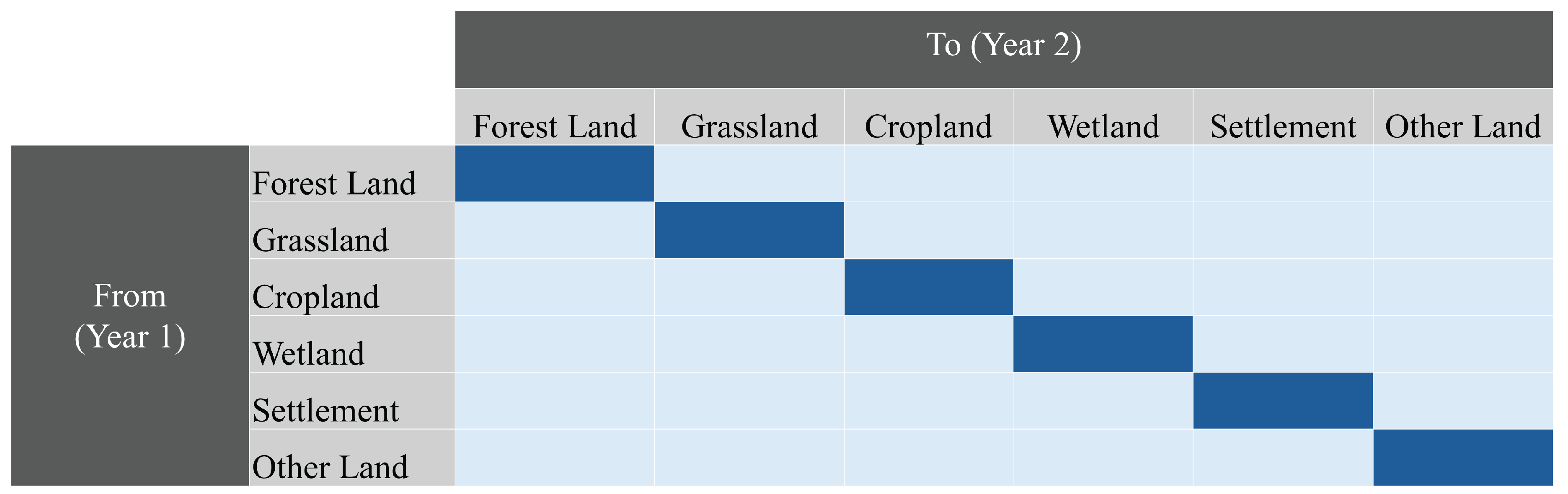
Figure 2.
Activity data categories from the IPCC land use transition matrix recategorized into GHG reporting categories. EF = emission factor; RF = removal factor; F = forest; NF = nonforest; TOF = trees outside forest; F>F = forest remaining forest; F>NF = forest to nonforest; NF>F = nonforest to forest. “RF” corresponds to activity data that are paired with a removal factor, and “EF” corresponds to activity data that are paired with an emission factor.
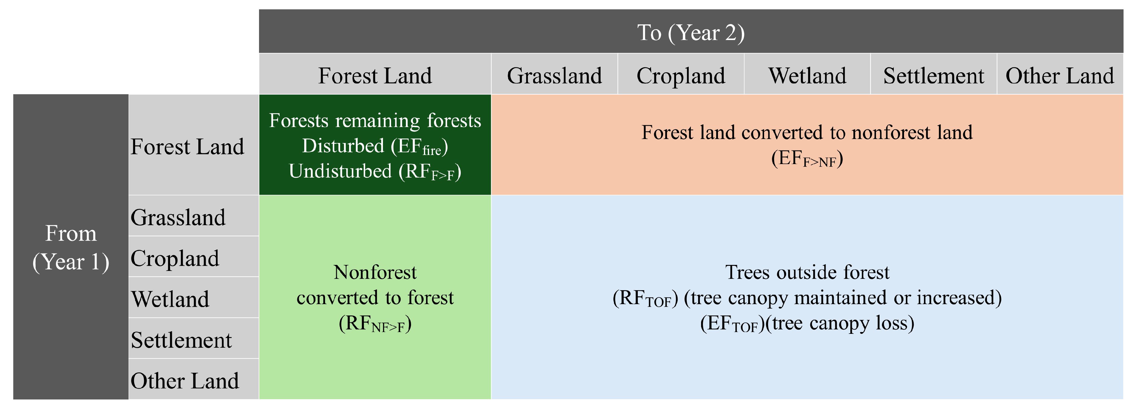
Figure 3.
Summary of emissions and removals for four successive time periods in Jefferson County, Washington. Stacked columns show gross emissions (positive values) and gross removals (negative values) by inventory period. Purple columns represent the overall net flux for the inventory period. All values are annual averages across the inventory period. All units in Mg C/year.
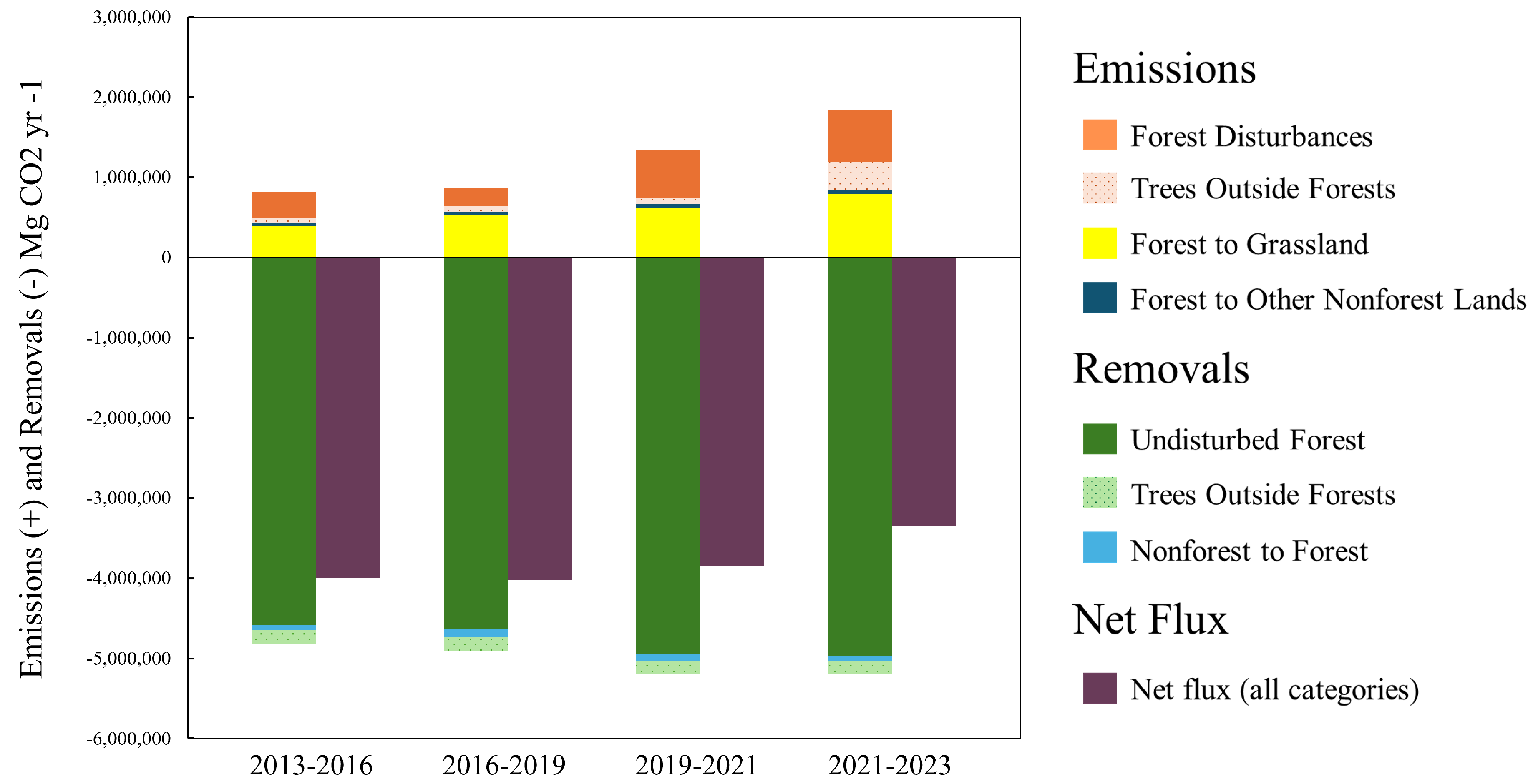
Figure 4.
Forest-to-grassland change and harvest disturbance (2019–2021) in Jefferson County. (a) County outline (cyan) with the zoom frame for panel (b) in orange. (b) Detail showing forest-to-grassland conversion (light orange) and harvest/other disturbance (dark orange). The legend applies to both panels.
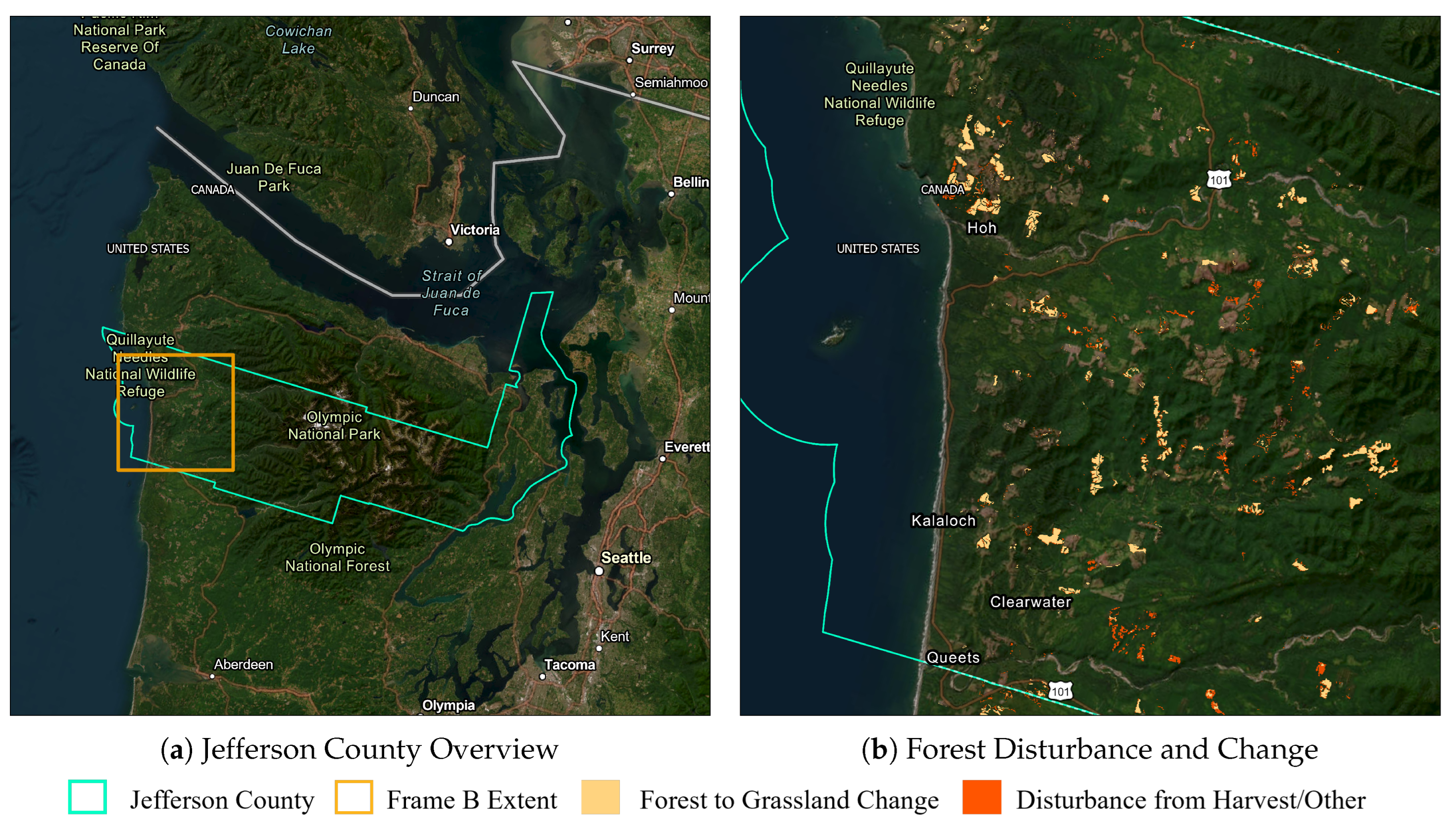
Figure 5.
Summary of emissions and removals for four successive time periods in Montgomery County, Maryland. Stacked columns show gross emissions (positive values) and gross removals (negative values) by inventory period. Purple columns represent the overall net flux for the inventory period. All values are annual averages across the inventory period. All units in Mg C/year.
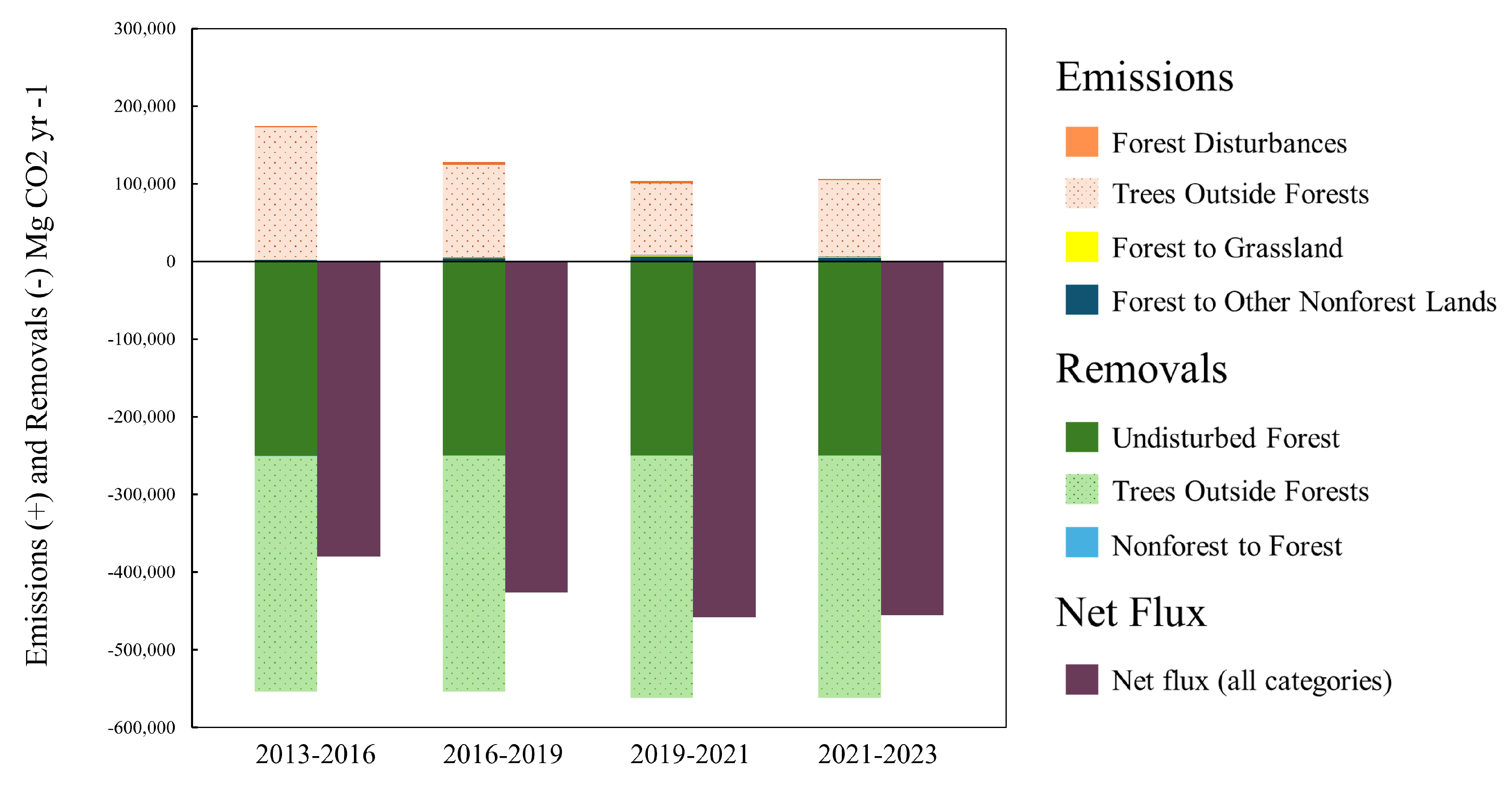
Figure 6.
Non-forest tree-canopy cover and canopy loss (2013–2016) in Montgomery County. (a) County outline (cyan) with the zoom frame for panel (b) in orange. (b) Detail showing tree-canopy cover (green gradient, 0–100 %) and gross canopy loss (orange gradient, 0–100 %) at 30 m resolution. The legend applies to both panels.
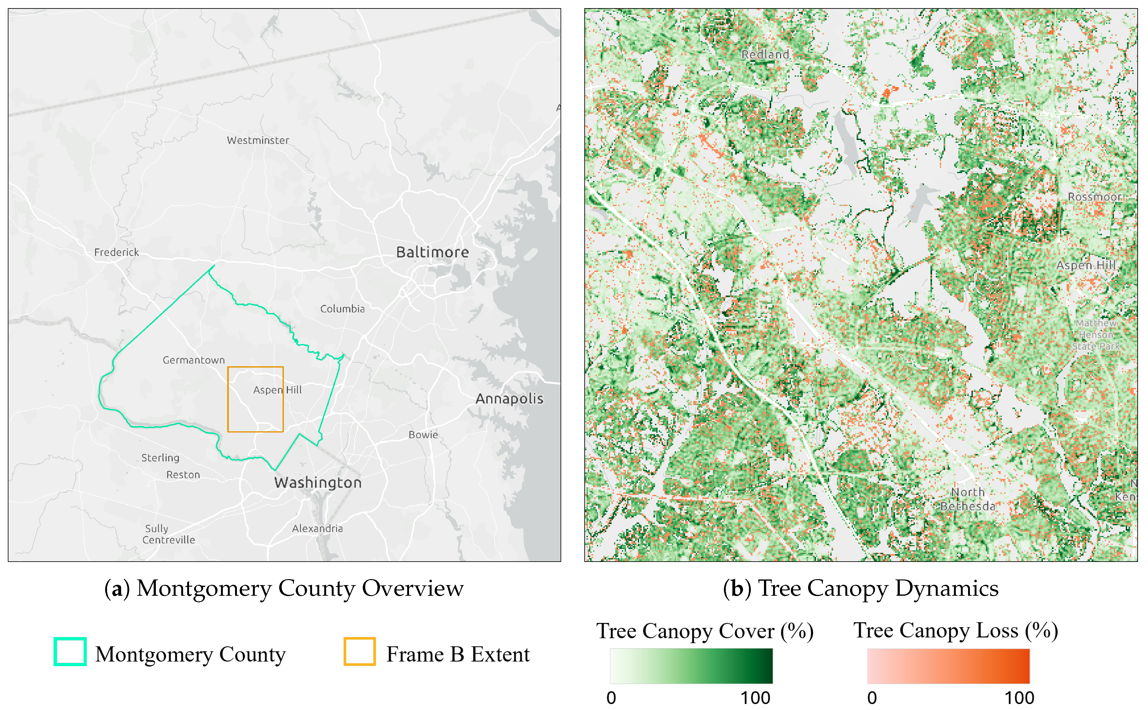
Figure 7.
Emissions from forest disturbances and removals from undisturbed forests in four successive time periods for all federally owned forests in CONUS. Stacked columns show gross emissions (positive values) and gross removals (negative values) by inventory period. Purple columns represent the overall net flux for the inventory period. All values are annual averages across the inventory period. All units in Mg C/year.
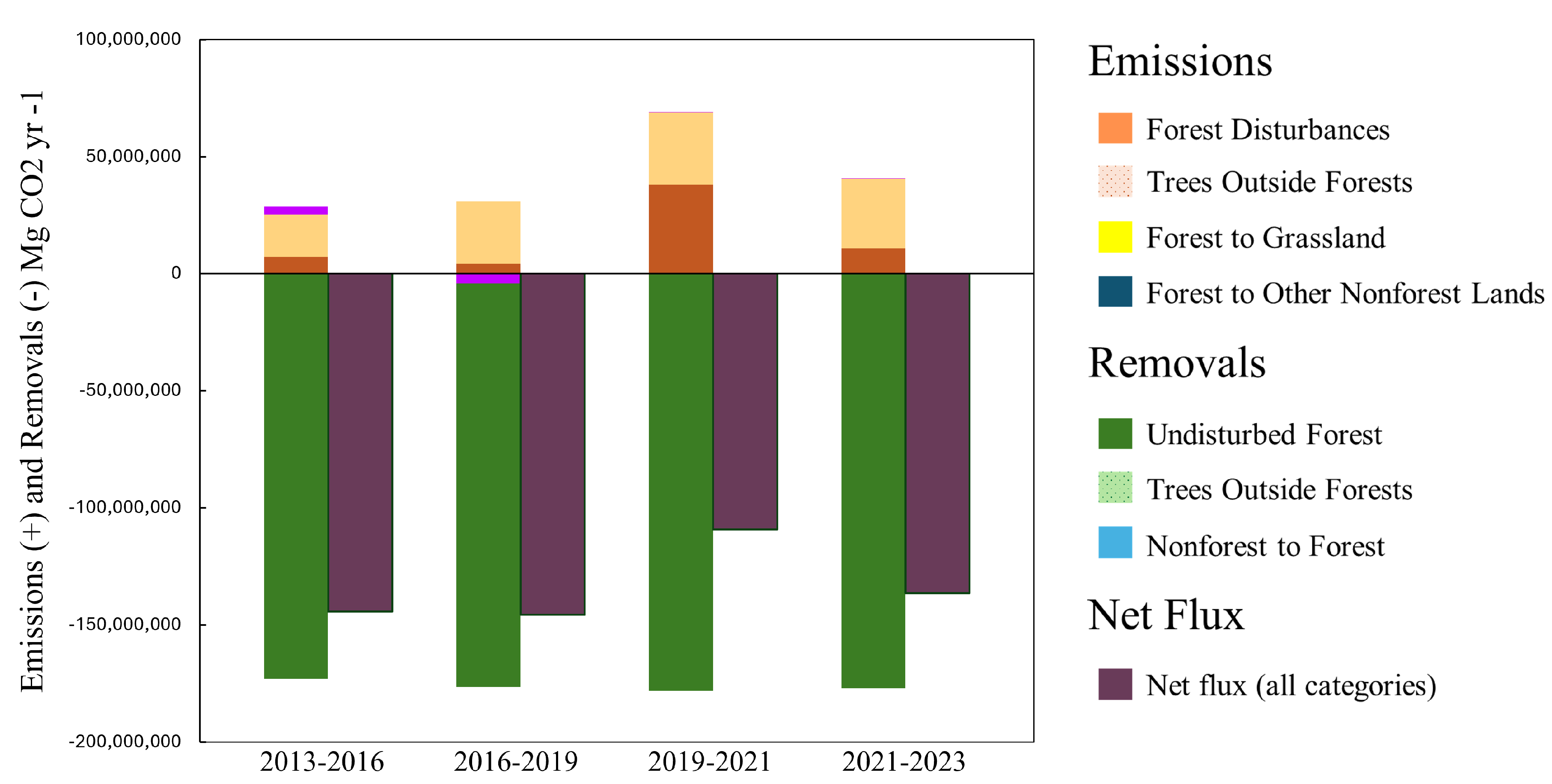
Figure 8.
Disturbance categories on federally owned forests (2013–2023). (a) Continental-US view with the zoom frame for panel (b) in cyan. (b) Detail showing undisturbed forests (green) and disturbances (fire = brown, harvest/other = orange, insect/disease = purple). The legend applies to both panels.
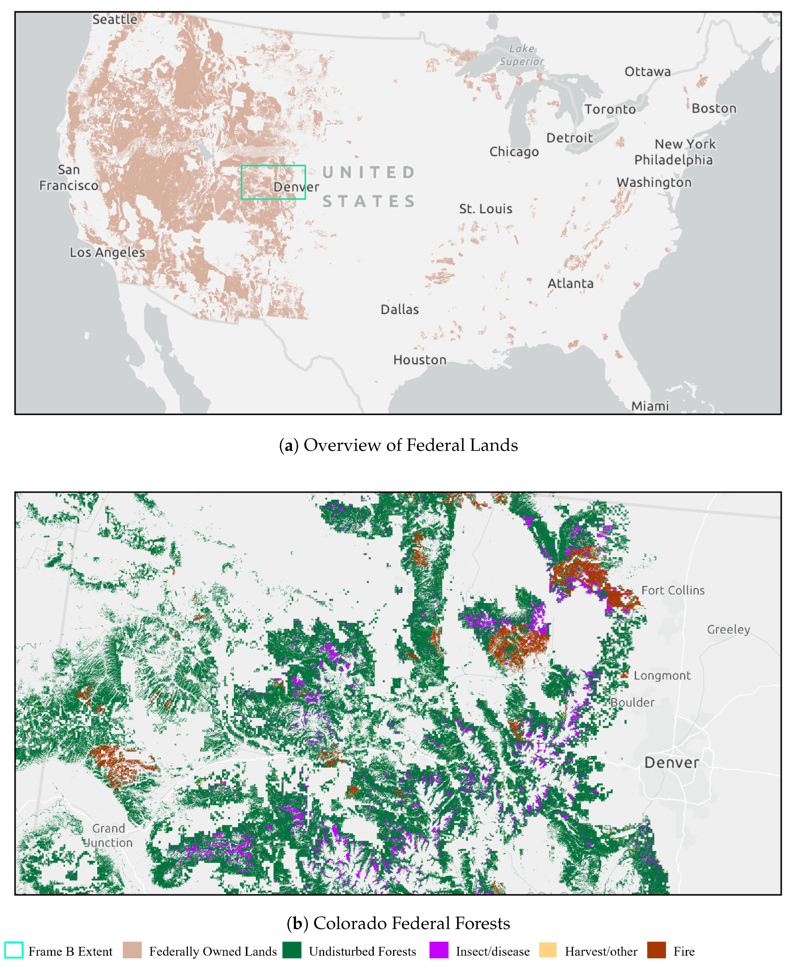
Table 2.
Greenhouse gas inventories for four successive time periods in Jefferson County, Washington. Area units are in ha, and flux units are in Mg C/year. Positive values are gross emissions, and negative values are gross removals, except in the total Net Flux line, which is the sum or all emissions and removals per inventory period. All values are annual averages across the inventory period.
| 2013–2016 | 2016–2019 | 2019–2021 | 2021–2023 | |||||
|---|---|---|---|---|---|---|---|---|
| Category | Area | Flux | Area | Flux | Area | Flux | Area | Flux |
| Forest Change | ||||||||
| To Forest | 4,862 | –67,644 | 7,181 | –102,224 | 5,430 | –78,037 | 4,717 | –65,397 |
| To Cropland | 0 | 0 | 0 | 0 | 0 | 0 | 0 | 0 |
| To Grassland | 5,851 | 397,840 | 5,677 | 533,030 | 2,645 | 619,481 | 3,182 | 792,061 |
| To Other | 42 | 5,109 | 20 | 4,477 | 40 | 13,973 | 10 | 3,537 |
| To Settlement | 87 | 12,413 | 109 | 13,399 | 33 | 6,397 | 42 | 9,155 |
| To Wetland | 322 | 29,910 | 155 | 26,467 | 122 | 27,970 | 210 | 43,567 |
| Forest Remaining Forest | ||||||||
| Fire | 477 | 41,890 | 17 | 1,478 | 0 | 0 | 484 | 66,616 |
| Harvest/Other | 1,325 | 271,996 | 2,064 | 425,303 | 1,848 | 590,065 | 1,843 | 588,617 |
| Insect/Disease | 22,557 | –377,125 | 18,572 | –193,646 | 0 | 0 | 0 | 0 |
| Undisturbed | 354,328 | –4,580,890 | 356,932 | –4,635,858 | 380,079 | –4,951,419 | 381,584 | –4,973,477 |
| Trees Outside Forest | ||||||||
| Maintained/gained | 16,333 | –168,885 | 15,971 | –165,141 | 15,788 | –163,251 | 14,887 | –153,933 |
| Tree-canopy loss | 558 | 65,502 | 643 | 75,471 | 484 | 85,268 | 1,975 | 347,263 |
| Total Emissions | 447,535 | 885,979 | 1,343,154 | 1,850,816 | ||||
| Total Removals | –4,817,419 | –4,903,223 | –5,192,707 | –5,192,807 | ||||
| Net Flux | –4,369,884 | –4,017,244 | –3,849,553 | –3,341,991 | ||||
Table 3.
Greenhouse gas inventories for four successive time periods in Montgomery County, Maryland. Area units are in ha, and flux units are in Mg C/year. Positive values are gross emissions, and negative values are gross removals, except in the total Net Flux line, which is the sum or all emissions and removals per inventory period. All values are annual averages across the inventory period.
| 2013–2016 | 2016–2019 | 2019–2021 | 2021–2023 | |||||
|---|---|---|---|---|---|---|---|---|
| Category | Area | Flux | Area | Flux | Area | Flux | Area | Flux |
| Forest Change | ||||||||
| To Forest | 96 | –693 | 85 | –609 | 66 | –474 | 83 | –599 |
| To Cropland | 7 | 181 | 6 | 202 | 4 | 225 | 6 | 117 |
| To Grassland | 32 | 203 | 38 | 717 | 22 | 1,444 | 28 | 1,551 |
| To Other | 0 | 0 | 0 | 13 | 0 | 0 | 0 | 0 |
| To Settlement | 92 | 1,603 | 87 | 4,093 | 43 | 6,493 | 40 | 4,655 |
| To Wetland | 10 | 115 | 17 | 157 | 18 | 255 | 6 | 144 |
| Forest Remaining Forest | ||||||||
| Fire | 0 | 0 | 0 | 0 | 0 | 0 | 0 | 0 |
| Harvest/Other | 17 | 1,337 | 43 | 3,498 | 19 | 2,665 | 15 | 2,097 |
| Insect/Disease | 0 | 0 | 0 | 0 | 0 | 0 | 0 | 0 |
| Undisturbed | 38,398 | –249,973 | 38,319 | –249,456 | 38,340 | –249,592 | 38,328 | –249,520 |
| Trees Outside Forest | ||||||||
| Maintained/gained | 23,430 | –303,268 | 23,477 | –303,873 | 24,062 | –311,452 | 24,079 | –311,671 |
| Tree-canopy loss | 1,356 | 170,810 | 947 | 119,291 | 489 | 92,374 | 519 | 98,094 |
| Total Emissions | 174,249 | 127,971 | 103,456 | 106,658 | ||||
| Total Removals | –553,934 | –553,938 | –561,518 | –561,790 | ||||
| Net Flux | –379,685 | –425,967 | –458,062 | –455,132 | ||||
Table 4.
Greenhouse gas inventories for four successive time periods in federally owned forests in the forest remaining forest category. Area units are in ha, and flux units are in Mg C/year. Positive values are gross emissions, and negative values are gross removals, except in the total Net Flux line, which is the sum or all emissions and removals per inventory period. All values are annual averages across the inventory period.
| 2013–2016 | 2016–2019 | 2019–2021 | 2021–2023 | |||||
|---|---|---|---|---|---|---|---|---|
| Category | Area | Flux | Area | Flux | Area | Flux | Area | Flux |
| Fire | 160,102 | 7,186,885 | 91,328 | 4,178,937 | 429,712 | 38,001,265 | 116,570 | 10,810,266 |
| Harvest/Other | 198,490 | 18,023,850 | 267,781 | 26,788,129 | 185,121 | 30,936,174 | 174,497 | 29,760,304 |
| Insect/Disease | 3,699,556 | 3,615,148 | 2,896,261 | –4,256,666 | 201 | 3,369 | 483 | 5,806 |
| Undisturbed | 46,840,576 | –173,071,224 | 47,003,598 | –172,334,863 | 48,752,295 | –178,174,491 | 48,394,716 | –177,105,604 |
| Total Emissions | 28,825,883 | 26,710,400 | 68,940,808 | 40,576,376 | ||||
| Total Removals | –173,071,224 | –172,334,863 | –178,174,491 | –177,105,604 | ||||
| Net Flux | –144,245,341 | –145,624,463 | –109,233,683 | –136,529,228 | ||||
Table 5.
Comparison of LEARN and FIA area and net flux estimates. Area units are in ha, and flux units are in Mg C/year. Net Flux which is the sum or all emissions and removals per inventory period. For Jefferson County and Montgomery County, values are annual averages for the 2019-2021 period. Values exclude trees outside forests, but include forests remaining forests and forest change. For Federal Forests, values are annual averages for the 2013-2023 period. Inventory periods were chosen to best align with FIA measurement dates. Values include forests remaining forests only.
| Case Study | LEARN Area | FIA Area | LEARN Net Flux | FIA Net Flux |
|---|---|---|---|---|
| Jefferson County | 390,712 | 384,469 | -3,875,242 | -3,966,447 |
| Montgomery County | 38,566 | 38,440 | -242,288 | -629,448 |
| Federal forests | 49,802,822 | 76,224,457 | -133,908,179 | -129,009,128 |
Disclaimer/Publisher’s Note: The statements, opinions and data contained in all publications are solely those of the individual author(s) and contributor(s) and not of MDPI and/or the editor(s). MDPI and/or the editor(s) disclaim responsibility for any injury to people or property resulting from any ideas, methods, instructions or products referred to in the content. |
© 2025 by the authors. Licensee MDPI, Basel, Switzerland. This article is an open access article distributed under the terms and conditions of the Creative Commons Attribution (CC BY) license (http://creativecommons.org/licenses/by/4.0/).
Copyright: This open access article is published under a Creative Commons CC BY 4.0 license, which permit the free download, distribution, and reuse, provided that the author and preprint are cited in any reuse.


