Submitted:
13 May 2025
Posted:
14 May 2025
You are already at the latest version
Abstract
Dredging of fine sediments and dumping of fines at disposal sites produce passive plumes behind the dredging equipment. Each type of dredging method has its own plume characteristics. All types of dredging operations create some form of turbidity (spillage of dredged materials) in the water column, depending on: i) applied method (mechanical grab/backhoe, hydraulic suction dredging with/without overflow); ii) nature of the sediment bed and iii) hydrodynamic conditions. A simple parameter to represent the spillage of dredged materials is the spill percentage (Rspill) of the initial load. In the case of cutter dredging and hopper dredging without overflow, the sediment spillage is mostly low with values in the range of 1% to 3%, The spill percentage is higher in the range of 3% to 30% for hopper dredging of mud with intensive overflow. Spilling of dredged materials also occurs at disposal sites. The spill percentage is generally low with values in the range of 1% to 3% if the load is dumped through bottom doors in deep water creating a dynamic plume which descends rapidly to the bottom with cloud velocities of 1 m/s. The most accurate approach to study passive plume behaviour is the application of a 3D-model, which however is a major, time-consuming effort. A practical 1D-plume dispersion model can help to identify the best parameter settings involved and to do quick scan studies. The proposed 1D-model represents equations for dynamic plume behaviour as well as passive plume behaviour including advection, diffusion and settling processes.
Keywords:
turbid plumes
; sediment plumes
; plume dispersion
; dynamic and passive plumes
Introduction
Turbid plumes (jets) carrying fine sediments (< 63 µm) are well known phenomena at the fresh-water outlet of a river into a coastal sea, at dredging/disposal/dumping sites and around beach nourishment sites in estuaries and coastal seas. Natural coastal plumes generated by river outflow (rainfall-runoff events) are different from dredging-dumping related plumes because of the fresh-water flows involved spreading the natural turbidity as surface flows along the coast and across the inner continental shelf and are highly susceptive to wind and wave-related forcings, whereas dredging-related primary plumes are more strongly mixed over the water depth by (tidal) currents. Secondary plumes are generated indirectly by resuspension of previously deposited materials of low bulk density (fresh deposits) during conditions with wind-induced waves and/or relatively strong tidal currents.
Dredging of sediments (clay, silt and fine sand particles/flocs) from harbour basins and approach ship-channels is known as maintenance dredging creating passive primary plumes behind the dredges (mostly hopper dredges). Beach nourishment of sandy sediments (including a fine fraction) from hopper-dredge unloading operations also produces passive primary plumes, but of smaller size and lower visibility as only minor fractions of fines are involved. The three essential elements of dredging are: excavation, transport and disposal. Often, the most critical elements are the excavation and the disposal (dumping) of sediments at the disposal site causing environmental pollution problems. In many cases the dredged material has to be dumped in the outer estuary or at open sea creating a dynamic plume/cloud descending to the sea bottom from which a passive plume of spilled materials is separated by turbulent vortices. Each type of dredger has its own plume characteristics. Cutter suction dredging (CSD) produces plumes near the cutter head, trailing suction hopper dredging (TSHD) creates plumes near the suction head and along the vessel due to overflow processes of fines. Grab/backhoe dredging creates plumes around the bucket, but are generally of minor size if a closed clamshell bucket is used. Dredging-related turbidity plumes require monitoring by remote sensing methods in combination with flow measurements and water sampling in order to document plume behaviour and water quality of local waters.
Ideally, the best approach for accurate plume dispersion modelling is the application of a 3D plume dispersion model (Teeter et al., 1999 [1] ; Moritz et al., 1999 [2]; Smith et al., 1999 [3]; Luger et al., 1998 [4], 2002 [5]; Li and Ma, 2001 [6]; Fernandes et al., 2021 [7]; Warrick et al., 2025 [8]). The input of fines (mud) is specified as a mud discharge (kg/s) in a certain cell at a fixed location. These studies show that the disposal of sediment in the water column and the plume behaviour (spatial and time-dependent evolution of the sediment concentrations) can be very well simulated by using a 3D-numerical model package based on the mass and momentum equations for the fluid and sediment phases. The fine sediment concentration are carried away by advective processes and are diluted by diffusive processes and settling processes (settling velocity ws) resulting in sediment deposits. The turbulence can be modelled by using the buoyancy-extended k-ε equations. Li and Ma (2001) [6] have compared their model results to experimental results obtained in a flume concerning the deposition of sediments (0.13 mm) discharged continuously at the surface of the flowing water. Fernandes et al. (2021) [7] studied the plume behaviour at various open ocean disposal sites (southern Brazil) in interaction with coastal currents and waves using a 3D-model package. The dispersion plumes in the disposal sites were sensitive to the wind intensity and direction. The area of the disposal sites took around 4 days to recover from the dredging operations and reach the usual (background) suspended sediment concentrations. Warrick et al. (2025) [8] have examined the size and extent of turbid coastal plumes of fines produced by beach nourishment near Santa Barbara, California (USA) using remotely sensed imagery and 3D hydrodynamic and sediment transport model simulations. They have found that wave height, wind speed and direction, and sediment settling velocity have strong controls on the direction and extent of the turbid plumes. The plume length reduced from 5 km to 1 km using a settling velocity of 1 mm/s (coarse silt) instead of 0.1 mm/s (fine silt/clay). High waves cause longer plumes with higher concentrations. The transport of fines is mainly along the coast in the form of relatively narrow plumes due to wind and wave-generated longshore currents and large-scale oceanographic currents. Locant rip current cells cause offshore-directed plumes and sediment deposits at the inner continental shelf.
The setup, calibration and validation of these types of detailed 3D models is a major, time-consuming effort. For accurate results representing the detailed concentration profiles over the depth, it is of utmost importance to use many grid points over the water depth (> 10). As a result, the run times of these large-scale, 3D models may become excessive (days to weeks), especially for longer time scales (1 year). Furthermore, often many runs have to be executed to evaluate the influence of the many parameters involved. Using large-scale 3D-models, the modelling process may easily become unworkable at present computer power. A practical 1D-plume dispersion model (SEDPLUME1D-model) can help to identify the best parameter settings involved, which is the focus point of this paper. The basic objectives of the present paper are: 1) to develop a practical (easy to handle) 1D plume dispersion model for simulation of sediment concentrations, transport and sediment deposits by dynamic and passive plumes; 2) to include the most important sediment dispersion mechanisms (advection, mixing, settling of particles and flocs) and 3) to explore the effects of the key parameters involved (sensitivity computations). The semi-analytical model has a short user-friendly input file. It is a standalone model which can be setup quickly and produce results within a short period of time (0.5 to 1 hour) facilitating quick-scan studies on a desktop/laptop computer. The runtime is negligible and the output file can be imported in excel for easy plotting of results. Methods and models are briefly introduced in Section 2. Information of measured turbidity values at dredging and disposal sites is given in Sections 3 and 4. Detailed descriptions of dynamic and passive plume behaviour of the SEDPLUME1D-model including calibration/ validation and practical cases are given in Sections 5 and 6. Conclusions are given in Section 7.
2. Methods and Models
A combination of methods and models is utilized in this paper: 1) analysis of many field studies to get information of the turbidity values (measured suspended sediment concentrations SSC) at the dredging/disposal sites (source locations) and 2) application of one dimensional and three-dimensional models for simulation of plume dispersion process. Turbidity is caused by the actual dredging/excavation process at the sediment bed (resuspension effect); the spillage during filling of the dredge/barge (overflow); the spillage during horizontal transportation from dredging to dumping site and the spillage during unloading of the vessel/barge at the disposal site. The operation of plume dispersion models require detailed knowledge of the turbidity values generated during dredging and dumping activitie (for input of data).
Two models are herein used to simulate the plume dispersion processes: 1) the numerical DELFT3D modelling package and the semi-analytical SEDPLUME1D-model. The process-based DELFT3D hydrodynamic and sediment transport model (Deltares 2018 [9]; Lesser et al. 2004 [10]) consists of various submodules: water levels and currents, waves and suspended sediment transport forced with in-situ observations of current velocity, wave data and spill discharges at source locations. The computational model domain consists of a structured, orthogonal curvilinear grid covering the bathymetry aera of interest. The primary goal of the 3D simulations is to generate plume behaviour data (suspended sediment concentrations) which can be used for calibration/validation of the simple SEDPLUME1D-model.
The semi-analytical SEDPLUME1D-model is a one dimensional model which represents both dynamic and passive plume behaviour. The dynamic plume behaviour is based on the mass and momentum equations for a high-concentration sediment mixture (sediment cloud of fine and coarse materials). Basic input parameters are the initial cloud size, cloud velocity and cloud concentration which are strongly related to the cloud release characteristics of the dredging vessel involved. The passive plume behaviour describing the far-field concentrations is based on longitudinal and lateral mixing, vertical settling process and gradual exponential adjustment of the suspended sediment concentrations to equilibrium values. Five sediment fractions are included with basic input parameters being: fraction size, settling velocity and suspended sediment concentration (source concentration) and the relevant flow characteristics (flow depth and depth-averaged velocity).
3. Turbidity Caused by Dredging Processes
3.1. General Aspects
Turbidity (or SSC) is the expression used to describe the cloudy or muddy appearance of water. Turbidity instruments measure the presence of particles indirectly through their optical properties or directly by taking water samples. The standard unit of measurement for turbidity is the Nephelometric Turbidity Unit (NTU) measured with a nephelometer in a standard suspension of formazin in water. Roughly, the SSC (in mg/l) is 50% of the NTU-value. All types of dredging operations create some form of turbidity in the water column, depending on the: i) applied dredging method (mechanical grab, bucket dredging; hydraulic dredging including overflow); ii) nature of the sediment bed and iii) hydrodynamic conditions. The two most turbidity generating dredging methods are: grab dredging and hopper dredging. In the case of grab dredging, the leakage of fines and resuspension are caused by: a) the bed impact; b) the vertical movement of the bucket through the water column; c) the movement of the bucket from the water to the barge. In addition, losses of sediment can occur if the barge is allowed to overflow. In the case of hopper dredging, the sediment leakage occurs by: a) suction losses around the suction mouth; b) filling to overflow level and b) overflow of excess water forced out of the hopper resulting in low concentrations (≅1 kg/m3) at the start of the overflow process and high concentrations (≅100 kg/m3) at the end of the overflow process (Van Rhee, 2002 [11]; Spearman et al., 2011 [12]). In fine sandy conditions, the total overflow generally is of the order of 5% to 10% (Van Rhee, 2002 [11]). In muddy conditions, the overflow can reach values up to 30% of the total volume of sediment pumped into the hopper and may cause significant environmental problems (Van Parys et al., 2001 [13]). The high-concentration overflow slurry may descend towards the bed as a dynamic plume. Simultaneously, a passive low-concentration plume is generated in the water column by mixing/entrainment processes along the surface of the high-concentration slurry. The descending slurry eventually collapses onto the bed to form a density current propagating and settling out along the seabed over some distance (< 100 m). The passive plume is slowly diluted/dispersed in the ambient current by advection, lateral mixing and settling out of sediments to the bed.
3.2. Turbidity Values Measured at Field Dredging Sites
Various field studies have been performed to analyse the turbidity values produced during dredging activities (Wakeman et al., 1975 [14]; Stuber, 1976 [15]; Bernard, 1978 [16]; Sosnowski, 1984 [17]; Hayes et al., 1984 [18]; Willoughby and Crabb,1983 [19]; Blokland, 1988 [20]; Pennekamp and Quaak, 1990 [21]; Kirby and Land, 1991 [22]; Pennekamp et al., 1991 [23]; Pennekamp, 1996 [24]; Dankers, 2002 [25]; Winterwerp, 2002 [26]; Battisto and Friedrichs, 2003 [27]; LACS (Los Angeles Contaminated Sediments) Task Force, 2003 [28]; Clarke et al.,2007 [29]. A detailed overview of field data is given by Mills and Kemp 2016 [30]). The results of these studies are summarized in Table 1. The results are expressed in the following four basic parameters: 1) depth-averaged background concentration (C); 2) increase of depth-averaged concentration (ΔC) at a distance of 50 m from centre of dredging activity; 3) decay time (ΔT) of the increase of the concentration after cessation of dredging activity; time after which the depth-averaged turbidity has diminished to background values at 50 m from dredging centre; and 4) spill, loss or resuspension parameter Sspill, which is the dry mass of sediment brough into suspension per m3 of dredged material.
The Sspill-parameter is defined as:
Sspill=Mspill/Vinsitu=Mspill/(Minsitu/ρdry,insitu)= ρdry,insituMspill/Minsitu=ρdry,insitu (Rspill/100)
The production of spill (kg/s) is related to the dredging production (m3/s), as follows:
Pspill=Sspill Pinsitu=ρdry,insitu (R/100) (Pinsitu)
with: Mspill= dry mass of spilled sediment brought into suspension (kg); Mdm=total insitu mass of sediments to be dredged out (kg); Vinsitu=Volume of sediments to be dredged out (m3); ρdry,insitu= in-situ dry density of sediment to be dredged (before dredging); ρdry,pumped= α ρdry,insitu= dry bulk density of pumped sediment (during/after dredging in pump line, kg/m3); α=factor (0.3-0.5); Rspill=Mspill/Minsitux100%=100Sspill/ρdry,insitu =spill percentage=spill percentage of dry sediment mass (1% to 10%); Sspill= dry sediment mass (kg/m3) lost for each m3 of in-situ (source) material dredged out; Pinsitu= production of dredging equipment of in-situ volume (m3/s); Ppumped =[ρdry,insitu/ρdry,pumped]Pinsitu =volume production rate of (added) water + sediment material (m3/s); Pspill= production rate of spill of fines brought into suspension (input for dispersion models). Spill-values and Rspill-values of various dredging methods are given in Table 1 (data from literature). The initial spill concentration at the dredging (source) location can be determined in two ways: 1) ratio of spill mass (kg) and water volume around vessel (≅3 water displacement volume; m3) and 2) ratio of spill production/flux (kg/s) and water discharge (bhu in m3/s; b=width, h=depth, u=depth-averaged flow velocity ) carrying spill away from source.
Becker et al. (2015) [31] have proposed generic formulations for the source terms related to dredging and dumping of sediments. Their method is based on soil characteristics and dredge production rates, combined with empirically derived, equipment and condition specific source terms. The parameters involved are: 1) the
total mass and volume of fines to be dredged (kg) and 2) the dry density of in-situ sediments and the fraction of particles < 63 μm. The production rate of a dredger is formulated as the dredged in-situ volume per unit time, which is the ratio of the in-situ volume to be dredged (m3) and the product of number of days with dredging work, the number of loadings per day (24 hours) and the loading time of dredger (seconds). For example, the cycle time of a hopper dredger consists of: loading without overflow (≅ 0.5 hr) + loading with overflow (≅ 1 hr) + sailing to dump location (≅ 1 to 5 hrs) + dumping of load (≅ 0.1 hr) + sailing to dredging location (≅1 to 5 hrs) giving a total time of 3 to 12 hrs. In the case of hopper dredging, there are losses at the dredging site due to the loading (suction) processes and the overflow processes and losses at the dumping site. The losses (mass) are estimated using efficiency coefficients or spill coefficients (e = efficiency or spill factor; eloading = 0.01-0.03; eoverflow = 0.1-0.5; eplume = 0.1-0.3 based on experience). The spill flux (kg/s) is the mass of the spill divided by the time duration involved. The spill concentration can be derived from the flux divided by the water discharge carrying the spill mass away from the source.
The effectivity of the dredging process can be evaluated from the dry mass of dredged sediment derived from the pre- and post-bathymetric surveys and the dry mass of sediment passing through the pump line of the dredger. This can be formulated, as follows:
ρdry,insitu (- Vbed change)= ρdry,pumped Qmixture Δtpump αe
{(ρwet,insitu - ρw)/αs} Vbed change= {(ρwet,pumped - ρw)/αs} Qmixture Δtpump αe
-Vbed change= {(ρwet,pumped - ρw)/(ρwet,insitu - ρw)} (Qmixture Δtpump αe)
αe= -Vbed change/[{(ρwet,pumped - ρw)/(ρwet,insitu - ρw)} (Qmixture Δtpump)]
αe = -Vbed change/Vpump
with:
Vbed change=volume of removed water and sediment based on pre- and post-bathymetric surveys (negative if bed at t2 lower than at t1 and positive if bed at t2 higher than at t1); generally the bed change volume is negative at most dredging sites;
Vpump= {(ρwet,piumped - ρw)/(ρwet,insitu - ρw)} (Qmixture Δtpumped) =volume of water and sediment through pump line;
Qmixture= pump discharge of dredger involved; Δtpump= total pump time; ρwet,insitu=wet density of in-situ material; ρwet,insitu=wet density of pumped mixture (range of 1200-1300 kg/m3); αs=(ρs - ρw)/ρs= coefficient
αe= effectivity coefficient (range 0.5-0.9).
αe<1 if Vpump >-Vbed change; in case of heavy natural infill during dredging and/or infill from overflow or side-casting processes in the period between the pre- and post surveys.
αe>1 if Vpump <-Vbed change; in case of natural scour or removal of in-situ sediment by propeller action of moving vessels in the period between the pre- and post surveys.
αe<0 means that the bed is higher at t2 despite the dredging efforts which can only occur in conditions with intensive natural siltation and/or strong return flow of dredged materials (dump site too close to dredging site).
JanDeNul Dredging Group (JDN) has derived the effectivity factor (αe) from the dredging and survey data of a ship-channel project in Bangladesh, neglecting the siltation contribution (Van Rijn, 2023). The αe-values are in the range between 0.3 and 0.6 based on survey-data. The error involved is most likely relatively small in the dry season when natural siltation is relatively small. The αe-factors in the dry season are in the range of 0.4 to 0.6. The αe-factors of the monsoon period of about 0.4 are rather low because siltation is high.
LACS (Los Angeles Contaminated Sediments) Task Force (2003) [28] has analysed the available data (40 to 50 cases) on the loss of sediments during dredging operations without overflow from various dredging studies in the USA and from the literature. Figure 1 shows the cumulative probability distribution of the loss/resuspension coefficient Rspill (%) on the horizontal axis of hydraulic (without overflow) and mechanical dredging methods.
It is shown that hydraulic dredging methods tend to resuspend less sediment into the water column than do mechanical dredging methods. To include the uncertainties involved, it is wise to use the 90%-values. For example: Rspill, 90% = 3% for hydraulic dredging, which means that in 90% of the studied cases, the R-factor was < 3% and in 10% > 3%. The R90% value is a factor of 5 (mechanical) to 10 (hydraulic) higher than the R50% value. The Rspill-parameter (derived from water samples) of hydraulic dredges represent the spill of fines at some distance (10 to 30 m) from the dredging point which are washed away by local currents. The Rspill-values close to the dredging point may be much higher (5% to 10%) but most of the coarser spilled sediments will settle immediately close to the dredging point (within 30 m).
Figure 2 shows the measured suspended sediment concentrations (above the background concentrations) at a distance of about 30 m from the dredge point based on data summarized by the LACS Task Force (2003) [28]. The R90% value is a factor of 3 (mechanical) to 10 (hydraulic) higher than the R50% value. The turbidity concentrations produced by mechanical dredging methods are, on average, larger than those produced by hydraulic dredging methods. This may be caused by the fact that turbidity concentrations caused by mechanical dredging are generated at almost any point in the water column.
4. Turbidity Due to Dumping Processes
4.1. General
The method of dumping used most strongly depends on the potential environmental effects. At most sites, the turbidity due to the dumping processes should be minimum requiring low spillage disposal methods. Most of the disposed materials will sink relatively quickly to the bed as a density current. The silts and clays spilled in the water column are generally dispersed over relatively large areas in the presence of currents. In shallow water, the deposited sediments can be stirred up easily in relatively shallow water by wind waves. The thickness of the deposits at the dump site should remain relatively small (not more than 10% of local water depth) at the end of the project to minimize resuspension. Preferably, the disposal site should be selected at a location where the wave and current-related bed-shear stresses remain relatively small so that the sediments are not dispersed or carried away from the designated limits of the site (Scheffner, 1991 [32]). The available dumping methods are:
free fall dumping (bulk load) using hopper or barges with bottom doors or split hull hopper/barges;
continuous plume disposal by pumping of mixture through a floating or submerged pipe into the water column;
side casting at disposal site; sediment is pumped from the hopper into the water column;
side casting at dredging site using a side casting dredger (with or without a special boom), which directly pumps the dredged sediments into the water as far as possible away from the dredger; this is very efficient in situations with very weak tidal currents (lagoons) or unidirectional cross-currents away from the dredging site; or at sites with excessively high siltation rates;
continuous free fall disposal from a spray boat; often used in shallow water to make land reclamations by spraying thin layers of sand on the bottom and to minimize the spreading of turbidity.
4.2. Free Fall Loads Through Bottom Doors
Fine sediments are released from hopper dredgers in the form of a high-concentration slurry of water and sediments (concentrations of the order of 300 to 600 kg/m3) through bottom openings on a time scale of 1 to 10 minutes. In the case of a split hull barge or hopper, the hull of the vessel splits open to release the load almost instantaneously. After release, the behaviour of dredged materials strongly depends on the sediment (cloud) concentrations during exit discharge, as follows:
high-concentration dynamic plume; dredged materials of high concentration behave as a (negatively buoyant) sediment cloud moving towards the seabed where it forms a density current radiating outwards from the point of impact; a minor amount of the fines (<3%) are striped from the cloud during descent and are dispersed in the water column and carried away as a passive plume;
low-concentration passive plume: dredged materials of low concentration are discharged through a pipe exit or are striped off from the high-concentration cloud and behave as a passive plume of sediments affected by local current velocities and turbulent mixing processes resulting in rapid dilution of the plume and rapid dispersal of fines in the water column and settling of particles onto the bed.
Descent
Quick release dumping of dredged materials in shallow water < 100 m from a hopper dredger falls in the category of dynamic jets/plumes and consists of three phases (Bokuniewicz et al., 1978 [33]; USACE 2015 [34]; Mills and Kemp, 2016 [30]):
convective descent: dredged materials descent as a big and coherent cloud of sediment to the seabed under influence of gravity (excess density) with a velocity far greater than the settling velocity of the individual fines; shear stresses developing along the interface between fluid and sediment cloud cause local turbulent eddies which entrain fluid into the cloud and sediment out of the cloud reducing the excess density (lower cloud concentrations) and increasing the volume of the cloud; fines are stripped/separated from the cloud by turbulent eddies resulting in suspended spill concentrations in the water column;
dynamic collapse into density current after impact onto the seabed and radiating outwards with decreasing horizontal velocities; fines are stripped from the density plume and mixed into the overlying water as suspended spill;
passive spreading and transports by local currents if the dynamic plume is sufficiently diluted (only in very deep water).
Bokuniewicz et al. (1978) [33] have studied the dumping process at various sites in the USA using echo-sounding equipment and various electronic sensors for velocity and concentrations. Their data show that the descent speed of a high-concentration cloud of fines is in the range of 1 to 3 m/s and strongly depends on the insertion speed which is the initial speed of the cloud after release from the dredger. The descent speed roughly is 0.4 to 0.8 times the insertion speed. The water depth has not much effect on the descent speed as long as the cloud is not disintegrated and behaves as dynamic plume (descent speed >> settling speed of individual cohesive particles/flocs/aggregates). The insertion speed can be derived from the emptying rate (discharge rate) and the open door area of the hopper. The emptying rate depends on the type of dredged materials in the hopper load (density, load thickness), the geometry and opening speed of the bottom doors. The insertion speed can to some extent be controlled by the dredge operator (door opening speed or area). A high insertion speed can be used to reduce the transit time (and minimize spill) to the seabed in conditions with a strong current and/or large depth. A low insertion speed can be used to increase the transit time resulting in a smaller bed impact and bed surge.
An important process during descent of the high-concentration sediment cloud (slurry) to the seabed is the entrainment of water into the cloud due to the generation of a thin boundary layer flow with shear stresses along the interface of the cloud producing small-scale turbulent eddies which bring clear water into the cloud and sediment out of the cloud into the boundary layer. By this entrainment and dilution processes with clear ambient water, the cloud volume of water and sediment increases strongly during descent, but at the same time the bulk cloud density decreases due to dilution. Bokuniewicz et al. (1978) [33] measured the lateral spread due to entrainment by using horizontally scanning echo-sounding equipment and found that the cloud volume impacting the seabed was 70 times greater than the initial released volume at a site with depths up to 45 m. In very deep water, there is a relatively long descent path and thus more water can be entrained mixed into the descending cloud resulting stronger dilution. Spill of fines (2% to 3% of the initial load) along the interface of the cloud may occur during the descent of the cloud. The spill is somewhat higher (<3%) at dump sites with strong tide-/wind-induced currents > 0.7 m/s due to interaction of current-related turbulence with the descending cloud. Strong currents also cause significant (but predictable) displacement of the descending cloud, particularly in the zone where the cloud is decelerated sufficiently (to the velocity of the ambient current) and the cloud concentration is substantially reduced to values below 10 kg/m3 and gradually becomes a passive cloud. Monitoring of mud concentrations during dredging operations generally show low mud concentrations in the range of 100 to 200 mg/l in the passive trailing plume at about 100 m from the source (Wolanski et al., 1992 [35]; Healy et al. 1999 [36, 37]). Table 2 presents values of various dumping parameters for 2 modern hopper dredgers with bottom doors. The insertion speed varies in the range of 1 to 2 m/s for soft mud dredged materials (wet density of about 1250 kg/m3) depending on the number of doors, the total effective door area and the opening time. The effective door area is somewhat less than the opening area due to the presence of opening machinery and the doors are not completely vertical in full opening position. The insertion speed is relatively high (> 1 m/s) for a hopper (AVH) with many doors (high percentage of door area in relation to the total area). Hopper 1 (AVH) has 14 doors with a total effective door area of 210 m2, which is 23% of the load area. Hopper 2 (G) has 4 doors with maximum effective area of 80 m2.
Bed impact
At most field sites, the dredged materials reach the seabed while travelling at speeds < 1 m/s. The jet plume is deflected after bed impact and runs radially away in all directions as a disk-type of density current (or density surge) at speeds of 0.5 to 1 m/s over hundreds of meters before coming to rest. The initial thickness of the spreading disk with supercritical flow is 3 to 4 m carrying a sediment load with concentrations of about 10 kg/m3 and in the range of 1 to 5 kg/m3 near the surge front. In deeper water the cloud diameter is larger due to dilution processes resulting in a higher initial thickness (4 to 6 m), but with lower sediment concentrations (< 5 kg/m3). Both the thickness and the speed of the density current decrease at distances further away from the impact point with the sediments of the decelerating cloud gradually settling out.
4.3. Example of Predicted Turbidity Values at Dumping Sites Through Bottom Doors
The sediments (30% fines < 32 μm, 40% fines of 32-63 μm and 30% sand > 63 μm) are brought in the flow by direct dumping through bottom doors. The dry density of the sediment load is 400 kg/m3. The total volume of the load is 1000 m3. The dumping time is 600 s. The displaced water volume of the vessel (length x width x vessel draft) is Vdw=2100 m3. The fraction 32-63 μm (settling velocity=1.8 mm/s) will settle rapidly close to the dumping site. The fraction < 34 μm (settling velocity <0.45 mm/s) will remain in suspension.
The spill production is given by: Pspill=(Rspill/100) ρdry,sediment Pdump. Using: Rspill=2.5%, ρdry,sediment=400 kg/m3 and Pdump=1000/600=1.67 m3/s, it follows that Pspill= (2.5/100)x600x1.67=25 kg/s. The initial spill concentration can be determined from the spill mass and the volume of water around hopper (≅3Vdw) resulting in a spill concentration of Sspill/Vwater=0.025x1000x400/(3x2100) ≅1.5 kg/m3=1500 mg/l at the source location. The method of Becker et al. 2015 [31] yields similar values.
5. Modelling of Dynamic Plume Behaviour
5.1. General
The dynamic plume behaviour as implemented in the SEDPLUME1D-model is described in detail. Both the mass and momentum balance equations are considered. Calibration and practical cases are described.
5.2. Dynamic Behaviour of Mud Cloud from Hopper Vessel
A mud cloud with initial volume Vc,o and initial mud concentration cc,o is assumed to fall from the surface to the seabed. The cloud is assumed to consist of a series of cylinders with diameter D and height αD (α in the range of 1 to 2), cloud velocity (wc) and cloud density (ρc) released from the hopper vessel see Figure 3. The forces acting on the cloud are the gravity force (Fg), the buoyancy force (Fb), the drag (Fd) en the skin friction (Ff) forces. The diameter of each cylinder grows during descent of the cloud volume, as the cloud is gradually diluted due to entrainment of water into the cloud. The sediment mass (Mc) of the cloud is reduced by spill concentrations separated from the cloud by the action of vortices. In the case of shallow depth conditions, a turbidity current along the bed is generated (Van Rijn, 2004 [38])
Momentum balance cloud:
Mc dw/dt=∑F
ρc Vc dwc/dt = Fg - Fb - Fd - Ff
ρc Vc dwc/dt = ρc g Vc - αc ρw g Vc - 0.5 α1 ρw cD D2 wc2 - 0.125 α3 ρw D2 fw wc2
dwc/dt = g (ρc - αc ρw)/ρc - 0.5 (α1/α2)(ρw/ρc) (cD/D) wc2 - 0.125 (α3/α2) (ρw/ρc) (fw/D) wc2
Assuming dwc/dt =0 and no skin friction, the terminal fall velocity of a sphere is:
0.5 (α1/α2)(ρw/ρc) (cD/D) wc2 = g (ρc - ρw)/ρc
Using: α1= 0.25π≅0.75; α2=π/6 for a sphere, it follows that: wc2= cD-1 (4/3) [(ρc - ρw)/ρw] g D
which is the Stokes settling equation (Stokes, 1851 [39])
Volume and Mass balance of cloud:
dVc/dt= Qf,in - Qs,out
dVc/dt=ve (α6 As) - vs (α6 As) cc/ρs
dVc/dt= (ve - vs cc/ρs) (α6 α3 D2)
dMc/dt= -ms,out
dMc/dt= -vs (α6As) cc
Total loss of mass: Ms,out=∑(-Ms,out)
Percentage of mass loss with respect to initial mass: Ps,loss=(Ms,out/Mc,o)x100%
with: Mc= cc Vc = mass of sediment in cloud (Mc,o=Vc,o cc,o); cc= sediment concentration in cloud (=dry density of cloud, kg/m3); ρc =wet bulk density of cloud (kg/m3); ρw= fluid density (kg/m3); ρs= sediment density (2650 kg/m3); g= gravity acceleration (m/s2); wc= vertical cloud velocity (downward);
Vc=α2 D3=volume of core cloud (m3); α2=π/6=0.52 for sphere; α2=1 for cube; α2=π/4=0.79 for cylinder with h=D; α2=2π/4=1.57 for h=2D and α=3π/4=2.36 for h=3DAc=α1 D2=area of cross-section of cloud normal to velocity (m2); α1=0.25π=0.79 for sphere and cylinder; α1=1 for cube;
As=α3 D2= area of surface of cloud (m2); α3=π=3.14 for cylinder with h=D; α3=2π=6.28 for h=2D and α3=3π=9.42 for h=3D; α3=π=3.14 for sphere; α3=6 for cube; D= (Vc/α2)1/3=representative size (effective diameter) of core cloud (m); Fg= ρc g Vc = gravity force; Fb= ρw g Vc =buoyancy force; Fd= 0.5 ρw cD Ac wc2= 0.5 α1 ρw cD D2 wc2 = drag force; Ff = As τf = α3 D2 0.125 ρw fw wc2 = skin friction force; cD= drag coefficient (0.5 to 2); fw= skin friction factor (0.005 to 0.12); τf= shear stress; Qf,in = volume of water entering cloud due to dilution processes per unit time (m3/s); Qs,out= volume of sediment leaving cloud per unit time (m3/s);
ms,out= mass of sediment leaving cloud per unit time (kg/s); ve= entrainment velocity of water=α4 wc; α4= entrainment coefficient (0.05 to 0.1); vs= net loss velocity of sediment=α5 wc; α5= loss coefficient sediment (0.001 to 0.002); α6= reduction coefficient (most entrainment occurs at underside of the cloud (front) and lower part of cloud; range 0.7 to 0.8). The initial cloud diameter and cloud height strongly depend on the dimensions of the bottom door opening and the draught of the vessel.
Equations (4) and (5) are implemented in the SEDPLUME1D-model.
The field data set of the Rochester site in the fresh-water Lake Ontario in the USA (Bokuniewicz et al. (1978 [33]) has been used for calibration of the model, see Table 3andFigure 4. The water depth at the dump site is 15 m. The drag coefficient cD, the water entrainment coefficient α4 and sediment coefficient α5 were used as calibration parameters. The initial cloud diameter is set to 2 m and the initial cloud height is also set to 2 m (small scale barge). The best overall results are obtained for cD=2, α4=0.15; α5=0.001. The cloud velocity reduces from 2 m/s near the surface to about 0.7 m/s near the bottom, which is in good agreement with the measured velocity. The computed cloud concentration near the bed is about 15 kg/m3, which is of the right order of magnitude. Bokuniewicz et al. (1978 [33]) report values of 10 kg/m3 in the surge cloud further away from the dump impact point. The computed total sediment loss (spill) from the cloud is 2% of the initial sediment mass in the cloud (Rspill=2%)
Figure 5 shows an example of mud dumping by a hopper dredger in a coastal sea with a depth of 70 m and slurry density of 1250 kg/m3. The initial cloud diameter is set to 3 m (width of door opening). The initial height of the cloud is of the order of the hopper draught (≅6 m). The initial cloud velocity is set to 1 m/s. The fluid density at surface is 1020 kg/m3 linearly increasing to 1030 kg/m3 at bottom. The other model parameters are: drag coefficient=CD=3; skin friction coefficient=fw=0.05; entrainment velocity=ve=α5wc with α5=0.15; sediment loss coefficient α5=0.001. The cloud accelerates from 1 to 2.5 m/s within 2 sec and after that decelerates from 2.5 m/s near surface to 0.7 m/s at bottom (70 m below surface). The mud cloud concentration decreases from 300 kg/m3 near the surface to about 3 kg/m3 near the bottom. The mud cloud velocity close the bottom of 0.7 m/s is much higher than the local eddy velocity scale of about 0.1 m/s and also much higher than the settling velocity of individual particles/flocs (order of 1 mm/s), which means that the cloud cannot be effectively disintegrated by turbulent vortices. The cloud remains a dynamic plume down to the bottom (no passive behaviour), even in deep water with depth of 70 m. The dynamic behaviour is most pronounced in the upper 40 m of the water depth with downward mud cloud velocity > 1 m/s. The computed total sediment loss (spill) from the cloud is 3% of the initial sediment mass in the cloud (Rspill=3%).
6. Modelling of Passive Plume Behaviour and Dispersion
6.1. General Aspects
The passive plume behaviour as implemented in the SEDPLUME1D-model is described in detail. The model is based on diffusion-advection theory for depth-averaged parameters. Both longitudinal and lateral mixing processes are included. Four diverse validation cases are described and explained, including 3D-model dispersion results. Finally, a practical case concerning the plume generation and dispersion from cutter suction dredging is described in detail.
6.2. Theory of Diffusion/Dispersion/Dilution Processes
Basic equations
Generally, the modelling of passive types of plumes is based on the numerical solution of a diffusion type of equation in which the spreading or dispersal of the suspended sediment concentration is represented by the temporal and spatial gradients of the sediments concentrations in all directions Diffusive type of transport (εi ∂c/∂xi) is also known as Fickian transport. Dispersion refers to the spreading of the mass of fine sediments with a very small settling velocity (almost zero) as a bulk property (averaged concentrations) integrating all spreading/dispersion processes (K>>ε). Generally, the dispersion coefficient including all effects (K) is much larger than the turbulent mixing coefficient. The 2DV-dimensional vertical advection-dispersion process of fine sediments < 63 μm in a horizontally uniform flow (dh/dx=0, du/dx=0) can be described by:
∂c/∂t + u ∂c/∂x – ws ∂c/∂z – εz ∂2c/∂z2– εx ∂2c/∂x2 = 0
with: c= sediment concentration, u= flow velocity (constant in space and time), ws= settling velocity of sediment, ε= effective diffusion/mixing coefficient (assumed to be constant in space and time; about 0.1 to 10 m2/s; K= dispersion coefficient including other effects), x=longitudinal coordinate, z=vertical coordinate.
Neglecting the settling velocity (very fine clayey materials and dissolved pollutants) and vertical diffusive transport, Equation (6) can be expressed as:
∂c/∂t + u ∂c/∂x – εx ∂2c/∂x2 = 0
which is valid for depth-mean concentrations.
Assuming a fluid at rest (u= 0), the expression becomes:
∂c/∂t - ε ∂2c/∂x2 = 0
When a mass M (in kg/m2) is released at x= 0 at time t= 0 as a line source (per unit width) in a channel with constant depth h (channel width=1 m), the solution of the 1-dimensional diffusion equation is:
c= M/(4π ε t)0.5 exp[–{x/(4 ε t)0.5}2]
with: c= depth-mean concentration (kg/m3), t= time, ε = constant diffusion/mixing coefficient (m2/s).
Equation (9) can be used for a line release (source) of very fine sediments in a narrow river/creek (small depth and width) The cloud will be rapidly mixed over the depth and moves downstream as a gradually dispersing cloud. Vertical mixing is normally completed within a distance of 10 to 30 times the local water depth (10h to 30h; h=local water depth). The longitudinal elongation of the tracer-response cloud is defined as longitudinal dispersion. Continuity requires that: M = h –∞∫∞ c dx (in kg/m2). Using: x=ut, it follows that: M = h t1∫t2 uc dt = uh t1∫t2 c dt = q t1∫t2 c dt, with t1 and t2 referring to the leading and trailing edges of the cloud and cmax decreases with 1/x0.5.
Equation (9) represents a symmetrical solution with respect to the moving coordinate system (x’=local distance to centre of cloud; x= distance to point release location). Defining x = ut + x’ and thus x’= x-ut, it follows that:
c= M/(4π ε t)0.5 exp[–{(x-ut)/(4 ε t)0.5}2] =cmax exp[–{(x-ut)/(4 ε t)0.5}2]
with: cmax = M/(4π ε t)0.5= peak value of the concentration at x=ut. Thus: cmax =∝ at t= 0 and cmax decreases with 1/(ε t)0.5. The solution represents a Gaussian distribution, which reads as: y=[2πσ2]-0.5 exp{-(x-μ)2/(2σ2}.
This yields: 2σ2 = 4 ε t or ε = σ2/(2t). The diffusion coefficient can be determined from the travel time (Δt) between 2 stations and the standard deviation (σ) of the dispersed cloud size in longitudinal direction at both stations: ε =(σ22-σ12)/(2 Δt). The transport and dispersion of pollutants has been extensively studied in USA-rivers using fluorescent dyes as water tracers (Wilson 1968 [40], Kilpatrick and Wilson 1989 [41], Jobson 1996 [42]). If Fickian diffusion correctly represents the total longitudinal mixing in rivers, the maximum (peak) concentration decreases in proportion to the square root of time (cmax~t-βor cmax~x-βand β= 0.5; see Equation 9). Measured data show that the maximum (peak) concentration in natural rivers generally decreases more rapidly with time than predicted by the Fickian law. The presence of pools and riffles, dead zones, bends, and other channel and reach characteristics will increase the rate of longitudinal mixing and almost always yield a value of β greater than the Fickian value of 0.5. The value of β is approximately 1.5 for very short dispersion times and decreases to 0.5 for very long dispersion times (Jobson 1996 [42]). A dilution factor can be defined as:
γd= γd,longitudinal γd,lateral = cx/co
with: cx= concentration at location x and co= source concentration; γd- values in Table 4.
The dilution effect is relatively large close to the source because the longitudinal concentration gradient is relatively large resulting in a relatively large diffusive transport (ε ∂c/∂x). Further away from the source, the concentration gradient decreases and hence the diffusive transport decreases.
Example case 1: longitudinal mixing in a narrow channel
Equation (10) is shown in Figure 6 for a line source with M=10 kg/m2 (being a spike-type release of very fine clay-type sediment at x= 0 at t= 0; single release event). The width of the line source is the same as the width of the channel. The settling velocity of the fine sediment is assumed to zero. The flow velocity is u= 0.5 m/s, the horizontal diffusion/mixing coefficient is set to ε= 0.1 m2/s.
Figure 6 shows the gradual dispersion of the (fine sediment) mass M in horizontal direction away from the source at t = 5, 20 and 100 seconds. The maximum concentration (cmax) can be obtained for x=ut yielding: exp[–{(x-ut)/(4 ε t)0.5}2] = 1. The maximum concentration in the 1D case decreases as: cmax~(ε t)-0.5.
Table 4 shows some theoretical results based on Equation (10) for 4 values of the mixing coefficient.
The computed concentrations and dilution factors are very small for large dispersion coefficients (100 m2/s) due to strong longitudinal mixing. Most of the spreading occurs in the initial phase (over a small distance from the source location). Ideally, the ε-value can be determined from a dye tracer experiment in unidirectional flow with a constant velocity. In practice, dye tracer experiments are often done in river flow, where the velocities near the bottom and near the banks are smaller resulting in additional velocity gradients and mixing processes. The combined effect is known as the dispersion coefficient (K) in the range of 1 to 100 m2/s.
Example case 2: longitudinal dispersion in a river
In 1965, a large injection of 1800 kilograms of a dye solution was used to measure the travel time in a reach of 168 km (width of about 1 km) of the Mississippi River from Baton Rouge to New Orleans, Louisiana (Stewart, 1967 [43]). Several injection points with lateral spacing of about 200 m were used across the wide river to generate a line source equal to the flow width of the river (Wilson 1968 [40]). Using this approach, lateral mixing effects can be neglected. The average discharge was approximately 6700 m3/sec. The river width near Baton Rouge is about 1000 m. The travel time of the cloud between station 34 km and station 202 km was about 80 hours or a travel velocity of about 0.6 m/s (approximately the cross-section averaged flow velocity). The dye dilution was a factor of 4 between the station at 34 km and 202 km. Equation (10) was used to estimate the dye concentration. The total initial dye mass was 1800 kg or 1.8 kg/m using a river width of 1000 m. Assuming that the dye is released quickly (< 1 minute), the longitudinal distance covered by the flow is about 20 m resulting in M= 1.8/20 ≅ 0.1 kg/m2. Assuming a water depth of 10 m, the initial dye concentration is 0.1/10= 0.01 kg/m3= 10 mg/l. The best agreement between the observed and computed dilution (factor 4) is obtained for a dispersion coefficient of about K=150 m2/s.
Longitudinal dispersion and settling of fine sediments
A relatively simple longitudinal dispersion model for fine sediment particles with settling velocity ws from a continuous line source of mud in a turbulent flow with vertical mixing processes can be obtained by applying an exponential modelling approach. The adjustment of the depth-averaged sediment concentration in a channel of constant width can be approximated by:
dcx/dx= -ASVM(cx-cx,eq)
with: cx= depth-averaged sediment concentration (uniform over depth); ceq= depth-averaged equilibrium sediment concentration (input value); Q= fluid discharge in channel (constant width); Qs= c Q = sediment transport in channel (in kg/s); ASVM= adjustment coefficient (in m-1).
The adjustment factor (ASVM) has been determined from computed results for a wide range of conditions using a detailed 2DV-suspended transport model (Van Rijn 1987 [44], 2017 [45}), yielding:
with: γ=coefficient (standard value=0.3; range 0.1-0.5; higher value gives shorter settling distance, quicker adjustment); h= flow depth; ws= fall velocity of suspended sediment (input value); u*= bed-shear velocity due to currents (=umean g0.5/C); C= 5.75 g0.5 log(12h/ks)= Chézy coefficient; ks= effective bed roughness height of Nikuradse ( Van Rijn 2011 [46]); umean= depth-averaged flow velocity; Hs= significant wave height. The adjustment of the mud concentration proceeds relatively rapid in the presence of waves (see effect of Hs/h parameter). Higher ASVM-values (higher fall velocity, smaller bed-shear velocity, higher relative wave height) lead to a more rapid adjustment to equilibrium conditions.
ASVM= γ(1/h)(ws/u*)(1+2ws/u*)(1+Hs/h)2
Lateral mixing
A continuous mud release source with initial width bo will be spread out (diluted) due to lateral mixing and dispersion processes. Based on available knowledge (Jirka et al., 2004 [47]), the lateral spreading due to mixing processes in a river flow can be described by:
with: bo=width of mud source, bx= width at location x, x= longitudinal coordinate, β= 0.5 to 1 (default=0.5).
bx=bo+2xβ
Figure 7 shows a dredging-related plume. The plume width increases from about 10 m at the source location to about 70 m at x=500 m, which corresponds to a β-value of 0.5 to 0.6; b500=10+(2x500)0.6=73 m.
The dilution factor due to lateral mixing processes is: γd,lateral = bo/bx= 1/[1+(2/bo)xβ]
Table 5.shows dilution factors for β=0.5 and β=0.7.
Combined longitudinal and lateral mixing: SEDPLUME1D-model
The SEDPLUME1D-model is a practical (analytical) expression for exponential decay of the sediment concentrations (c) including longitudinal and lateral mixing. The basic equation reads, as:
with: Asvm=γ(1/h)(ws/u*)(1+2ws/u*)(1+Hs/h)2; co= concentration at x=0; ceq= local equilibrium concentration; flateral=1/{1+(2/bo)xβ}= lateral mixing effect factor; no lateral mixing for β=0; ftime= time factor= dump time/interval time; dump time= duration of dumping process; interval time= time between two successive dumps; bo= width of mud source (≅10 m); β = coefficient related to lateral mixing (range=0.5-0.7); ws= settling velocity; γ=calibration coefficient (standard value=0.3; range 0.1-0.5; higher value gives shorter settling distance, quicker adjustment). Equations (15) is implemented in the SEDPLUME-model for simulation of mud turbidity plumes and can be used for the simulation of the decrease of fine sediment concentrations from a line source or point source. Five sediment fractions are considered: fraction 125-250 μm with settling velocity ws=22 mm/s; fraction 63-125 μm with ws=6.5 mm/s; fraction 32-63 μm with ws= 1.8 mm/s; fraction 16-32 μm with ws=0.45 mm/s and fraction < 16 μm with ws=0.25 mm/s. The effect of a discontinuous source can be taken into account by the time-related factor ftime (≤1). The sediment transport of the SEDPLUME1D-model is computed as Qfines=u b h c. The SEDPLUME1D-model can be used for cases with or without lateral mixing. It is noted that the sediment disposal processes close to the dredger (<100 m) with high initial concentrations (>>1 kg/m3) and group-settling velocities (>> 10 mm/s) cannot be represented by Equation (15). The daily deposition rate of sediments (in m/day) follows from:
with: ρdry,fines = dry bulk density of deposited fine sediments; Δt= time step (=86400 s for 1 day).
c= ftime flateral [ceq + (co-ceq) exp(-ASVM x)]
Δzb,x= [α ws cx/ρdry,fines] Δt
The deposition rate can also be computed as:
with: Qs,x= bx cx u h= transport of fines at distance x, bx=bo+2xβ= width of plume at distance x.
Δzb= [(Qs,x-Qs,x-Δx) Δt]/[0.5(bx +bx-Δx) Δx ρdry,fines]
Both equations yield almost the same results for small values of Δx (< 1 m).
The total deposited volume of fines in the plume area is:
with: Qs,o= total transport of fines at x=0; Qs,L= total transport of fines at exit boundary (x=L).
Vdeposition= [Qs,L-Qs,o] Δt/ρdry,fines
5.3. Validation of SEDPLUME1D-Model
Four diverse validation cases are described hereafter:
Case 1: Settling behaviour of suspended sediments in a river;
Case 2: Plume dispersion due to mud dumping in a tidal river;
Case 3: Plume dispersion generated by cutter suction dredging, Abu Dhabi;
Case 4: Plume dispersion generated by beach nourisnment operations, The Netherlands.
- Validation case 1: Settling behaviour of suspended sediments in a river
The settling behaviour of the SEDPLUME1D-model in unidirectional flow conditions is compared to that of the more detailed 2DV settling behaviour of the SUSTIM1D-model (Van Rijn et al. 2024a,b [48, 49]) for overload conditions of suspended sediments (fine sediments with settling velocity of 1 mm/s) in a channel with steady flow (constant width), see Figure 8.
The upstream water depth is 10 m; the water depth of the downstream section is 15 m. The approach flow velocity is 1.35 m/s (steady flow; no tide). The flow velocity in the downstream section is 0.9 m/s. The bed roughness is 0.03 m. The fluid density is 1025 kg/m3. The computed sediment transport at the entrance (x=0) of the channel with water depth of 15 m is 22.5 kg/m/s (SUSTIM2DV-model). The depth-mean concentration is 22.5/(0.9x15)=1.67 kg/m3= 1670 mg/l. The computed equilibrium transport in the downstream channel section is 7.45 kg/m/s (SUSTIM2DV-model). The depth-mean equilibrium concentration is 7.45/(0.9x15)=0.55 kg/m3= 550 mg/l. The values co=1670 mg/l and ceq=550 mg/l are used in the SEDPLUME1D-model. Lateral mixing is set to zero. The mud transport of the SEDPLUME-model is computed as: qmud=u h c.
Figure 8 shows the results of the SUSTIM2DV-model and the SEDPLUME1D-model for overload conditions of sediment with settling velocity of 1 mm/s. The decay of the mud transport of both models shows good agreement, which means that the settling behaviour of the simple SEDPLUME1D-model is quite good for fine sediments.
- Validation case 2: Plume dispersion due to mud dumping in a tidal river
Mud is dredged by a hopper dredger from a tunnel trench in a tidal river (Scheldt River in Belgium, see Figure 9) and dumped at locations outside the trench. The water depth is 10 m and the mean flow velocity is 1 m/s. The bed material is predominantly fine sand. The maximum background mud concentration in the tidal river is about 300 mg/l. During flood, two dump sites are used: A at 8.5 km from trench, B at 3 km. During ebb, mud is only dumped at site B. The dredging vessel has a length of 100 m; width of 20 m and hopper volume of 5000 m3. The dump process takes about 5 to 10 minutes per 2 hours (cycle time).
The spill production (kg/s) can be computed from: Pspill=(Rspill/100) ρdry,sedimentPdump with Rspill=spill percentage (%), ρdry,sediment=dry bulk density (k/m3), Pdump=dump production (m3/s).
Using Rspill=2.5%; ρdry,sediment=600 kg/m3 and Pdump=5000/600=8.33 m3/s for a dump time of 10 minutes (600 s), it follows that Pspill=3/100x600x8.33=125 kg/s. The initial mud concentration of the mud cloud at the dumping site can be estimated by using:
Δcdump=(Rspill/100)x Mload/Vwater around hopper = (Rspill/100)x ρdry,sediment x Vhopper/Vwater around hopper with Rspill=spill percentage; Mload= dry mass of load; Vhopper = hopper volume (5000 m3); Vwater around hopper= mixing water volume around dredger (≅3 Vhopper ≅15000 m3); ρdry,sediment = dry density of mud load (≅ 400-800 kg/m3).
Using: Rspill=3%, ρdry,sediment = 600 kg/m3, it follows that the increase of the mud concentration at the dump sites is: Δcdump= 2.5/100x600x5000/15000 =5 kg/m3=5000 mg/l.
Two models (SEDPLUME1D and DELFT3D) have been applied to estimate the increase of the mud concentration at the tunnel trench location. The input data of the SEDPLUME1D-model are: bo= width of mud plume at dumpsite= 30 m; ftime= time factor= dump time/interval time= 10/120≅0.1; h= water depth= 10 m; u= depth-averaged velocity = 1 m/s; Initial concentration=5 kg/m3=5000 mg/l. Three sediment fractions are used in both models, see Table 6. The increase of the concentrations due to the dumping of mud at sites A and B is also shown in Table 6. Conservative results are obtained by the SEDPLUME-model for β=0.4 (lateral mixing effect) and γ=0.1. The highest mud concentration increase is about 100 to 120 mg/l at the tunnel trench location when mud is dumped at site B during flood flow resulting in extra maintenance dredging in the trench. The mud concentration increase is about 50 to 60 mg/l when mud is dumped at site A during flood flow. In reality, the mud concentration increase will fluctuate in time due to the intermittent dumping process (once every 2 hours) and the tidal variations. The values of the DELFT3D model are somewhat higher because the erosion of fresh mud from the bottom at the dumping sites is included.
- Validation case 3: Plume dispersion generated by cutter suction dredging, Abu Dhabi
A ship-channel near the coast of Abu Dhabi was deepened by cutter suction dredging (CSD). The tidal range is about 1 m. The tidal currents are fairly weak in the range of 0.3 to 0.9 m/s. The natural bed material in the vicinity of the channel is predominantly sand. The dredging works consisted of: a) cutter suction dredging (CSD) of hard bottom materials (rock; sandstone) in some channel sections and b) trailing suction hopper dredging (TSHD) of sandy bed materials in other channel sections. A substantial amount of fines was released into the channel area as a result of the cutter dredging operations. Fine sediments were also dispersed by the tidal currents over a larger area (of the order of 50 to 100 km2) with sensitive habitats. Sediment concentrations measured (4-11 November 2023) at various depths in the water column (water depth of 10 m) in the sediment plume were used for calibration of the dispersion models, see Figure 10.
The suspended sediments were in the silt range (16 to 32 µm). The silt concentration at 100 m from the CSD was about 100 ± 50 mg/l and about 3 mg/l at 600 m from the CSD. The computed sediment concentrations of the SEDPLUME1D-model are also shown in Figure 10. The input data are: h=10 m; bo=10 m (line source width); u=0.5 m/s, bed roughness ks=0.03 m; sediment size=25 µm with settling velocity of 0.5 mm/s. Best agreement was found for bo=10 m, β=0.6 and γ=0.3. The measured concentrations are slightly underpredicted for x<300 m and slightly overpredicted for x>300 m.
- Validation case 4: Plume dispersion generated by beach nourishment operations, The Netherlands
The plume dispersion from a pipeline exit for beach nourishment operations of fine sand (d50≅200 µm) in shallow water (depth≅1.7 m) at the landward side of the Texel barrier island in the Netherlands was studied using the DELFT3D model and the SEDPLUME1D-model. The local tidal range is about 2 m. The peak flood velocity is about 0.45 m/s (flood velocity from SW to NE). The peak ebb velocity is about 0.3 m/s (ebb velocity from NE to SW), see Figure 11.
The cycle time of the dredger bringing a load of fine sand (20,000 m3) to the beach is 12 hours. The dredger connects to a pipeline and pumps fine sand with inclusion of about 5% silts during about 3 hours (pump discharge of 2 m3/s; sediment concentration in pipeline of about 300 kg/m3). The sand deposited near the pipeline exit is distributed over the beach by bulldozers. A part of the silty materials (fraction 10 μm with settling velocity ws,10 um=0.075 mm/s) is washed away from the beach site as a plume dispersion. The spill production is given by Pspill=(Rspill/100) ρdry,sediment Ppump. Using Rspill=2.5%, ρdry,sediment =dry density of sediment in pipeline=300 kg/m3, Ppump=2 m3/s, it follows that Pspill=(2.5/100)x300x2=15 kg/s.
The silt concentration in the pipelne is about 15 kg/m3 (5%). The silt transport at the pipeline exit is discharge x concentration is 2x15=30 kg/s. Assuming that 50% of the silts are deposited within the sand matrix and 50% of the silts are washed away as spill, the spill production is 15 kg/s. Hence, a spill percentage of 2.5% is realistic. The DELFT3D-model is operated with 8 layers in vertical direction. The horizontal diffusivity is Kx=Ky= 10 m2/s. The vertical diffusivity is computed by the model from the hydrodynamics (Kz ≅ 0.01 m2/s). The spill rate of 15 kg/s is released in the upper cell (cell height=0.2 m; horizontal grid size=25 m; cell volume=25x25x0.2=125 m3) at 2.2 km from the south-west corner point and about 0.4 km from the coastline. The mud source is the exit (red dots; Figure 12) of the pump-pipeline connected to the hopper dredger vessel. Figure 11 shows the depth-averaged flow velocity and the mud/silt concentration of the silt fraction near the surface (at pump exit location) at the shallow source location (depth≅1.7 m). The silt/mud concentration varies over the tidal cycle in the range 2000 mg/l to 6000 mg/l (cmean≅ 4000 mg/l). The concentration in the bottom cell varies in the range of 100 mg/l to 300 mg/l (cmean≅ 200 mg/l). The concentration is maximum during the tidal slack periods when the flow velocities are almost zero (turning of horizontal tide) and minimum during the periods with significant flow velocities in the range of 0.3 to 0.4 m/s (maximum advection and dilution). The concentrations in the surface cell with the pump exit are much larger (factor 10) than those in the bottom cell, which is caused by the relatively small settling velocities of the fine sediments. Furthermore, the vertical mixing is relatively small because the flow velocities are small (0.3 to 0.4 m/s). The additional mixing due to the pump jet is neglected. In practice, the difference between the surface and bottom concentrations in shallow depth of about 2 m will be much smaller.
Figure 12 shows the mud cloud movement of the fraction 10 μm near the bottom along the coast from south-west to north-west during flood flow and back during ebb flow. The maximum mud concentration is < 100 mg/l at 750 m from mud source cell at surface. The maximum mud concentration is < 30 mg/l at 1500 m from the mud source, which is the natural background mud concentration.
The simplified SEDPLUME1D-model has also been used to simulate the dispersion of the silt fraction during ebb flow to SW for two values of the lateral mixing coefficient β=0.5 and β=0.7; see Table 7. The input concentration (≅2000 mg/l) at the source location is set equal to the tide-and depth-averaged concentration at the source location of the 3D-model. The flow velocity is set equal to the mean velocity of about 0.3 m/s during the ebb tide. Very good agreement is obtained for β=0.7. A smaller β-coefficient of 0.5 yields larger concentrations compared to those of the 3D-model. Summarizing, it is concluded that the dilution factor of the very fine fraction of about 10 μm is in the range of 1/10 to 1/20 over a distance of about 500 m; 1/20 to 1/30 over a distance of about 1000 m. The 3D-model results show that the lateral mixing of very fines is relatively strong at short distances from the mud source location.
5.4. Plume Dispersion of Cutter Suction Dredging in Coastal Sea
The cutter-suction dredging (CSD) of firm sediments (sandstone) in a ship-channel section with length Lch is considered. The diurnal tidal range is about 1 m. The associated production of fines per tide can be represented as a line source and initial concentration co,flood and co,ebb over 1 tidal cycle, see Figure 13.
The cutter work is done in 100 days for a length of Lch=3000 m. Hence, the daily cutter progress rate is 3000/100=30 m per day or 15 m per flood phase of 12 hours. The effective legth normal to the flow direction is 15x0.7=10.5 m during flood. The basic spill data are: Rspill=3%; Pinsitu=2500 m3/hour=0.7 m3/s (cutter sediment production); ρdry,insitu=1200 kg/m3. Using Equation (2), it follows that the spill production of the cutter-suction dredger (CSD) is Pspill= 1200x(3/100)x0.7=25 kg/s.
The local tidal cycle is represented as 2 periods (each with duration of 12 hours; diurnal tide of 24 hours; flood=12 hours; ebb=12 hours) with quasi-constant flow velocities uflood and uebb. The initial concentration co,flood at some distance (about 50 to 100 m) is computed as:
with: Pspill=production of fines <250 μm by cutting process (in kg/s); Tflood= duration of flood period (12 hours); Lcutter,flood= cutter progress along the channel during flood; Vwater,flood= (Lcutter,flood sinαflood) hflood uflood Tflood=water passing the cutter during flood period over the effective distance of the cutter during one flood period; Ls= effective length of line source normal to flow= Lch sinαflood; Lch= length of channel section (m); αflood= angle between channel axis and flood velocity vector (90o=flood velocity normal to channel axis); hflood= representative water depth (m); uflood= representative depth-averaged velocity during flood≅0.7upeak,flood. Similar expression can be derived for the ebb flow.
co,flood= Pspill Tflood/Vwater,flood
co,flood= Pspill Tflood/[(Lcutter,flood sinαflood) hflood uflood Tflood]= Pspill/[(Lcutter,,flood sinαflood) hflood uflood]
Using: Pspill=25 kg/s, Lcutter,flood=15 m, αflood= 45o, hflood=12 m, upeak,flood=0.7 m/s; uflood=0.5 m/s gives: co,flood=25/(15x0.7x12x0.5)≅0.4 kg/m3=400 mg/l.
The SEDPLUME1D-model is used with: hflood=12 m, uflood=0.5 m/s, ks=0.1 m; β=0.6, γ=0.3, bo=10.5 m, ftime=1.
The dispersion is computed for 5 sediment fractions with total initial concentration of 0.4 kg/m3=400 mg/l and the following subdivision: 5% fraction 125-250 μm: c1= 20 mg/l; 10% fraction 63-125 μm: c2= 40 mg/l; 30% fraction 32-63 μm: c3=120 mg/l; 40% fraction 16-32 μm: c4=160 mg/l; 15% fraction < 16 μm: c5= 60 mg/l. The results of the SEDPLUME1D-model as function of distance for the flood phase of the tidal cycle with duration of 12 hours (diurnal tide) are given in Figure 14 and Figure 15. The travel distance of a fluid particle with velocity of 0.5 m/s over the flood phase of 12 hours (diurnal tide) is 0.5 x12x3600 ≅ 20 km.
The most important results for a production rate of fines of 25 kg/s during the flood period are:
total plume width increases from 10.5 m at source to 300 m at 5 km from the cutter dredging site;
the sediment concentrations decrease to below 1 mg/l at 4 km from the source location; the fine sand and coarse silt fractions settle out within 1.5 km;
deposited sediment layer is about 0.05 m close to the cutter dredging site and decreases exponentially to less than 1 mm at a distance of 5 km;
total deposition volume in the plume area is about 1000 m3 over 5 km (based on dry density of 800 kg/m3).
In all, 100 flood plumes are generated over 100 days. Adjacent plumes partly overlap each other. The plume dispersion length reducing the sediment concentrations to about 1 mg/l (just measurable) is roughly 5 km. To estimate the total deposition during all flood periods over 100 days, an overall approach can be used. The total spill mass during 100 flood periods (flood duration=12 hours=43200 s) is 25 kg/s x 100 x 43200 s =108 106 kg. Using a dry bulk density of 800 kg/m3, the total spill volume is 135,000 m3, which is distributed over the plume area (roughly 2100 m at the source location and 2500 m at 5000 m from the source) resulting in a mean deposition layer of 135,000/[0.5(2100+2500)x5000]=0.011 m=11 mm. About 50 mm at the source location to about 1 mm at 5000 m from the source.
A similar approach can be followed for ebb flow conditions.
7. Summary and Conclusions
Dredging of sediments (clay, silt and fine sand particles/flocs) from harbour basins and approach ship-channels produces passive primary plumes behind the dredging vessel (mostly hopper dredges). Beach nourishment of sandy sediments (including a fine fraction) from hopper unloading operations also produces passive primary plumes, but of smaller size and lower visibility as only minor fractions of fines are involved. The three essential elements of dredging are: excavation, transport and disposal. Often, the most critical elements are the excavation and the disposal (dumping) of sediments at the disposal site causing environmental pollution problems. In many cases the dredged material has to be dumped in the outer estuary or at open sea creating a dynamic plume/cloud descending to the sea bottom from which a passive plume of spilled materials is separated by turbulent vortices. Each type of dredger has its own plume characteristics. Cutter suction dredging (CSD) produces plumes near the cutter head; trailing suction hopper dredging (TSHD) creates plumes near the suction head and along the vessel due to overflow processes of fines. Grab/backhoe dredging creates plumes around the bucket, but are generally of minor size if a closed clamshell bucket is used.
Turbidity (or SSC) measured by optical instruments and/or water samples is the expression used to describe the cloudy or muddy appearance of water. All types of dredging operations create some form of turbidity (spillage of dredged materials) in the water column, depending on the: i) applied dredging method (mechanical, hydraulic with/without overflow); ii) nature of the sediment bed (soil conditions) and iii) hydrodynamic conditions (water depth, mean currents, salinity, waves). The two most turbidity generating dredging methods are: grab dredging and hopper dredging with overflow. A simple parameter to represent the spillage of dredged materials is the spill percentage (Rspill) of the initial load. In the case of cutter dredging and hopper dredging without overflow, the sediment spillage is mostly low with values in the range of 1 to 3%, The spill percentage generally is high in the range of 3% to 30% in case of hopper dredging of mud with intensive overflow. Spilling of dredged materials also occurs at disposal sites. The spill percentage is generally low with values in the range of 1% to 3% if the load is dumped through bottom doors in deep water (coastal or ocean waters) creating a dynamic plume which descends rapidly to the sea bottom with cloud velocities of about 1 m/s.
The most accurate approach to study passive plume behaviour is the application of a 3D-model, which however is a major, time-consuming effort. Runtimes may be excessive, particularly for long-term predictions. A practical 1D-plume dispersion model (SEDPLUME1D-model) can help to identify the best parameter settings involved and to do quick scan studies. The 1D-model represents equations for dynamic plume behaviour (sediment dumping through bottom doors) as well as passive plume behaviour including advection, diffusion and settling processes.
Plume generation can be minimized by eliminating the overflow or by using special equipment (environmental dredging). Some types of dredges have been specially designed for this purpose: 1) auger dredgers using special equipment (rotating screw) to move material towards the suction head; 2) disc-cutter dredgers with a cutter head which rests horizontally and rotates its vertical blades slowly (consolidated silt and sand) and 3) scoop/sweep dredgers using special equipment to scrape the material towards the suction intake. Silt screens hanging in the water can be used at sites with weak currents and low waves.
Funding
This research received no external funding.
Data Availability Statement
All experimental data are available on request.
Conflicts of Interest
The authors declare no conflicts of interest. (no funding involved).
References
- Teeter, A.M. et al., 1999. Modelling the fate of dredged material placed at an open water disposal site in upper Chesapeake Bay, USA, p. 2471-2486. Coastal Sediments, Long Island, USA.
- Moritz, H.P., Kraus, N.C. and Siipola, M.D., 1999. Simulating the fate of dredged material, Columbia River, USA, p. 2487-2503. Coastal Sediments, Long Island, USA.
- Smith, G., Mocke, G. and Van Ballegoyen, R., 1999. Modelling turbidity associated with mining activity at Elizabeth Bay, Namibia, p. 2504-2519. Coastal Sediments, Long Island, USA.
- Luger, S.A., Schoonees, J.S., Mocke, G.P. and Smit, F., 1998. Predicting and evaluating turbidity caused by dredging in the environmentally sensitive Saldanha Bay, p. 3561-3575. 26th ICCE, Copenhagen, Denmark.
- Luger, S.A., Schoonees, J.S. and Theron, A., 2002. Optimising the disposal of dredge spoil using numerical modelling, p. 3155-3167. 28th ICCE, Cardiff, UK.
- Li, C.W. and Ma, F.X., 2001. 3D numerical simulation of deposition patterns due to sand disposal in flowing water, p. 209-218. Journal of Hydraulic Engineering, Vol. 127, No. 3.
- Fernandes, E., Da Silva, P., Gonçalves, G. and Möller, O., 2021. Dispersion plumes in open ocean disposal sites of dredged sediment. Water 13 (6): 808. [CrossRef]
- Warrick, J.A., Stevens, A.W. and Tehranirad, B., 2025. Coastal fine-grained sediment plumes from beach nourishment near Santa Barbara, California. Coastal Engineering Journal. [CrossRef]
- Deltares. 2018. Delft3D-Flow User Manual. version 3.15. Delft, The Netherlands.
- Lesser, G. R., J. A. Roelvink, J. A. T. M. Van Kester, and G. S. Stelling. 2004. Development and Validation of a Three-Dimensional Morphological Model. Coastal Engineering 51 (8–9): 883–915. [CrossRef]
- Van Rhee, C., 2002. On the sedimentation process in a trailing suction hopper dredger. Doc. Thesis, Faculty of Civil Engineering, Delft University of Technology, Delft, The Netherlands.
- Spearman, J., De Heer, A., Aarninkhof, S. and Van Koningsveld, M., 2011. Validation of the TASS system for predicting the environmental effects of trailing suction hopper dredgers. Terra et Aqua 14 (125), 14-22.
- Van Parys, M. et al., 2001. Environmental monitoring of the dredging and relocation operations in the coastal harbours in Belgium, MOBAG 2000, Proc. XVIth WODCON, Kuala Lumpur, Malaysia.
- Wakeman, T.H., Sustar, J.F. and Dickson, W.J., 1975. Impact of three dredge types compared in San Francisco District, p. 9-14. World Dredging and Marine Construction.
- Stuber, L.M., 1976. Agitation dredging: Savannah Harbour, p. 337-390. Dredging: Environmental effects and Technology. Proc. WODCON VII, San Francisco, USA.
- Bernard, W.D., 1978. Prediction and control of dredged material dispersion around dredging and open-water pipeline disposal operations. Technical Report DS-7-13, Dredged Material Research Program. USWES, Environmental Laboratory, Vicksburg, USA.
- Sosnowski, R.A., 1984. Sediment resuspension due to dredging and storms: an analogous pair, p. 609-618. Dredging and dredged material disposal, Vol. I, ed. by R.L. Montgomery and J.W. Leach. Proc. of Conf. Dredging, Florida, USA.
- Hayes, D.F., Raymond, G.L. and Mc Lellan, T.N., 1984. Sediment resuspension from dredging activities, p. 72-82. Dredging and dredged material disposal, Vol. I, ed. by R.L. Montgomery and J.W. Leach. Proc. of Conf. Dredging, Florida, USA.
- Willoughby, M.A. and Crabb, D.J., 1983. The behaviour of dredge generated sediment plumes in Moreton Bay, p. 182-186. Sixth Australian Conference on Coastal and Ocean Engineering, Gold Coast, 13-15 July.
- Blokland, T., 1988. Determination of dredging-induced turbidity. Terra et Aqua, No. 38.
- Pennekamp, J.P.S. and Quaak, M.P., 1990. Impact on the environment of turbidity caused by dredging. Terra et Aqua, No. 42.
- Kirby, R. and Land, J.M., 1991. The impact of dredging: a comparison of natural and man-made disturbances to cohesive sedimentary regimes. Paper B3, Proc. CEDA-PIANC Conference,Amsterdam, Netherlands.
- Pennekamp, J.P.S., Blokland, T. and Vermeer, E.A., 1991. Turbidity caused by dredging compared to turbidity by navigation. Paper B2, Proc. CEDA-PIANC Conference,Amsterdam, Netherlands.
- Pennekamp, J.P.S., 1996. Turbidity caused by dredging viewed in perspective. Terra et Aqua No. 64.
- Dankers, P., 2002. The behaviour of fines released due to dredging; a literature review. Hydraulic Engineering Section, Faculty of Civil Engineering and Geosciences, Delft University, Delft, The Netherlands.
- Winterwerp, J.C., 2002. Near-field behaviour of dredging spill in shallow water, p. 96-98. Tech. Note Journal of Waterway, Port, Coastal and Ocean Engineering, March/April.
- Battisto, G.M. and Friedrichs, C.T., 2003. Monitoring suspended sediment plume formed during dredging using ADCP, OBS and bottle samples. Coastal Sediments, Florida, USA.
- LASC Task Force, 2003. Literature review of effects of resuspended sediments due to dredging operations. Anchor Environmental CA, L.P. Irvine, California, USA.
- Clarke, D., Reine, K., Dickerson, C., Zappala, S., Pinzon, R. and Gallo, J. 2007. Suspended sediment plumes associated with navigation dredging in the Arthur Kill Waterway, New Yersey. WODCON XVIII, Orlando, USA.
- Mills, D. and Kemps, H., 2016. Generation and release of sediments by hydraulic dredging: a review. Report of Theme 2 - Project 2.1 prepared for the Dredging Science Node, Western Australian Marine Science Institution, Perth, Western Australia. 97 pp.
- Becker, J., Van Eekelen, E., Van Wiechen, J., De lange, W., Damsma, T., Smolders, T. and Van Koningsveld, M., 2015. Estimating source terms for field plume modelling. Journal of Environmental Management, Vol. 149, 282-293.
- Scheffner, N.W., 1991. A systematic analysis of disposal site stability, p. 2012-2026. Coastal Sediments, Seattle, USA.
- Bokuniewicz, H. J., Gebert, J., Gordon, R.B., Higgins, J.L., Kaminsky, P., 1978. Field Study of the Mechanics of the Placement of Dredged Material at Open-Water Sites. Prepared by Yale University for the US Army Engineer Waterways Experiment. Technical Report D- 78-79.
- USACE, 2015. Dredging and Dredged Material Management. US Army corps of Engineers. Engineering and Design. EM 1110-2-5025, 31 July 2015.
- Wolanski, E., Gibbs, R., Ridd, P. and Mehta, A., 1992. Settling of ocean-dumped dredged material, Townsville, Australia, p. 473-489. Estuarine, Coastal and Shelf Science, Vol. 35.
- Healy, T., Ipenz, M. and Tian, F., 1999. Bypassing of dredged muddy sediment and thin layer disposal, Hauraki Gulf, New Zealand, p. 2457-2470. Coastal Sediments, Long Island, USA.
- Healy, T., Mehta, A., Rodriquez, H. and Tian, F., 1999. Bypassing of dredged littoral muddy sediments using a thin layer dispersal technique, p. 1119-1131. Journal of Coastal Research, Vol. 15, No. 4.
- Van Rijn, L.C., 2004. Extreme transport of sediment due to turbidity currents in coastal waters. Proc. 29th ICCE, Lissabon, Portugal.
- Stokes, G. G., 1851. On the effect of the internal friction on the motion of pendulums, Transactions of the Cambridge Philosophical Society, 9, 8–106.
- Wilson, J.F. 1968. Time-travel measurements and other applications of dye tracing. IAHS Publication 76.
- Kilpatrick, F.A. and Wilson, J.F., 1989. Measurements of time travel in streams by dye injection. Publication USGS, USA.
- Jobson, H.E., 1996. Prediction of travel time and longitudinal dispersion in rivers and streams. Publication USGS, USA.
- Stewart, M.R., 1967, Time of travel of solutes in Mississippi River from Baton Rouge to New Orleans, Louisiana: U.S. Geol. Survey Hydrol. Invest. Atlas HA-260.
- Van Rijn, L.C., 1987. Mathematical modelling of morphological processes in the case of suspended sediment transport. Doctoral Thesis, Technical University of Delft, The Netherlands.
- Van Rijn, L.C., 2017. Principles of sedimentation and erosion engineering in rivers, estuaries and coastal seas. www.aquapublications.nl.
- Van Rijn, L.C., 2011. Principles of fluid flow and surface waves in rivers, estuaries, seas and oceans. Aqua Publications, The Netherlands (wwww.aquapublications.nl).
- Jirka, G.H. et al., 2004. Management of point source discharges into rivers. International Journal River Basin Management, Vol. 2, No. 3, 225-233.
- Van Rijn, L.C.; Meijer, K.; Dumont, K.; Fordeyn, J. 2024. Practical 2DV modelling of deposition and erosion of sand and mud in dredged channels due to currents and waves. J. Waterw. Port Coast. Ocean. Eng. 2024, 150, 04024002. [CrossRef]
- Van Rijn, L.C.; Meijer, K.; Dumont, K.; Fordeyn, J., 2024. Simulation of sand and mud transport processes in currents and waves by time-dependent 2DV model. Int. J. Sediment Res. 2024, 40, 1–14. [CrossRef]
Figure 1.
Probability distribution (vertical) of Rspill-percentage (horizontal).
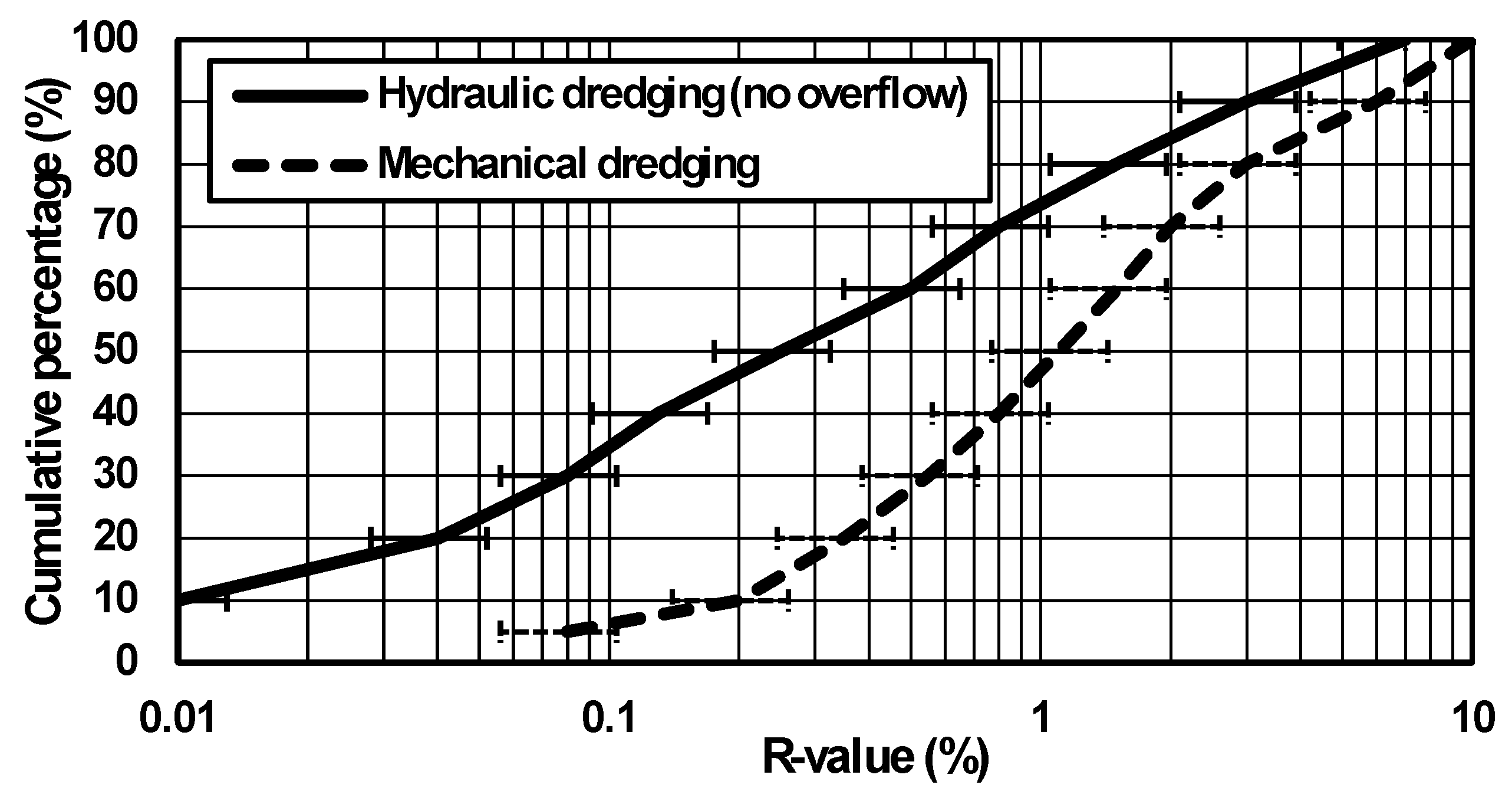
Figure 2.
Probability distribution of turbidity concentrations at 35 m from dredger.
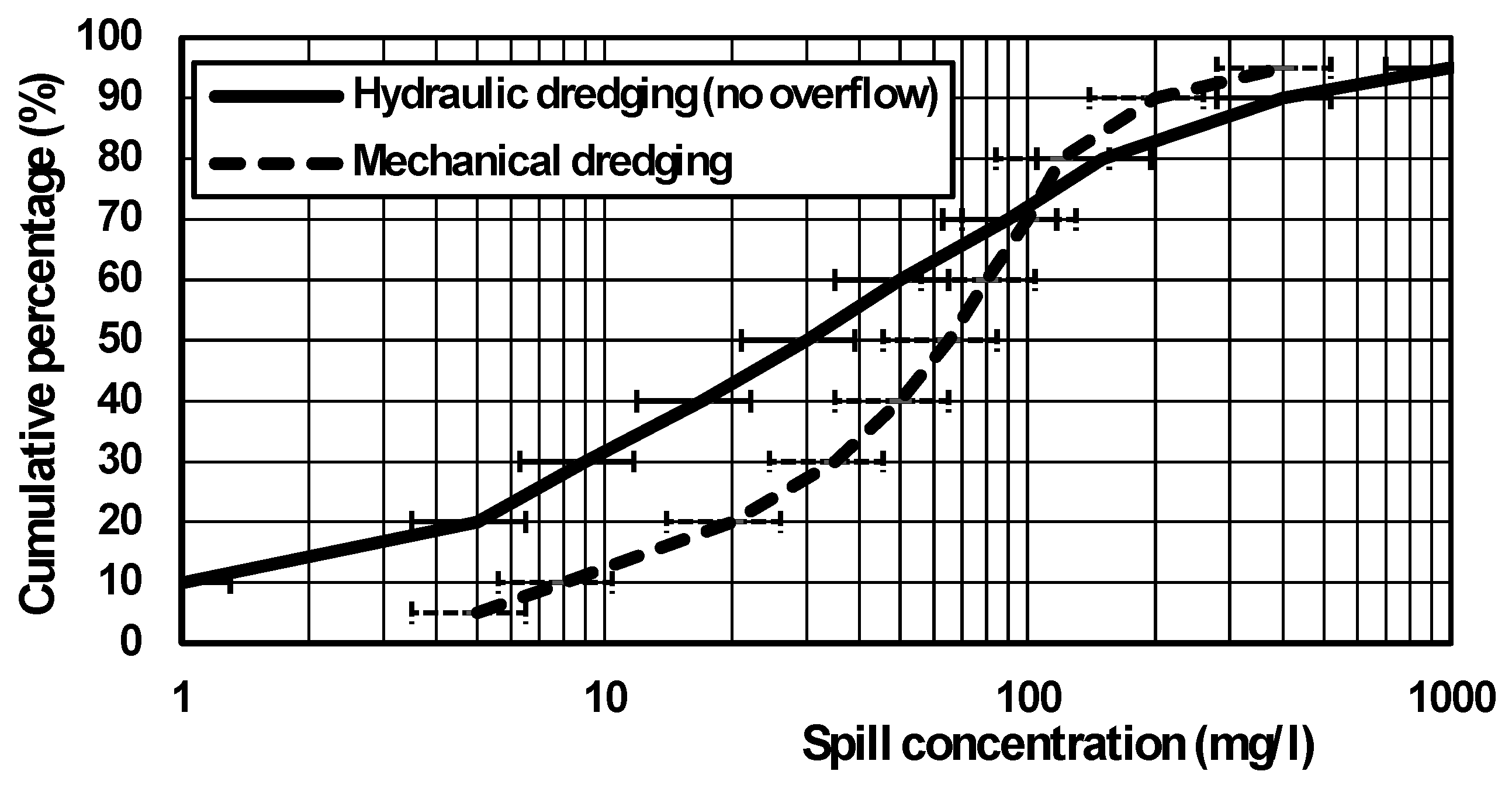
Figure 3.
Falling mud cloud schematization.
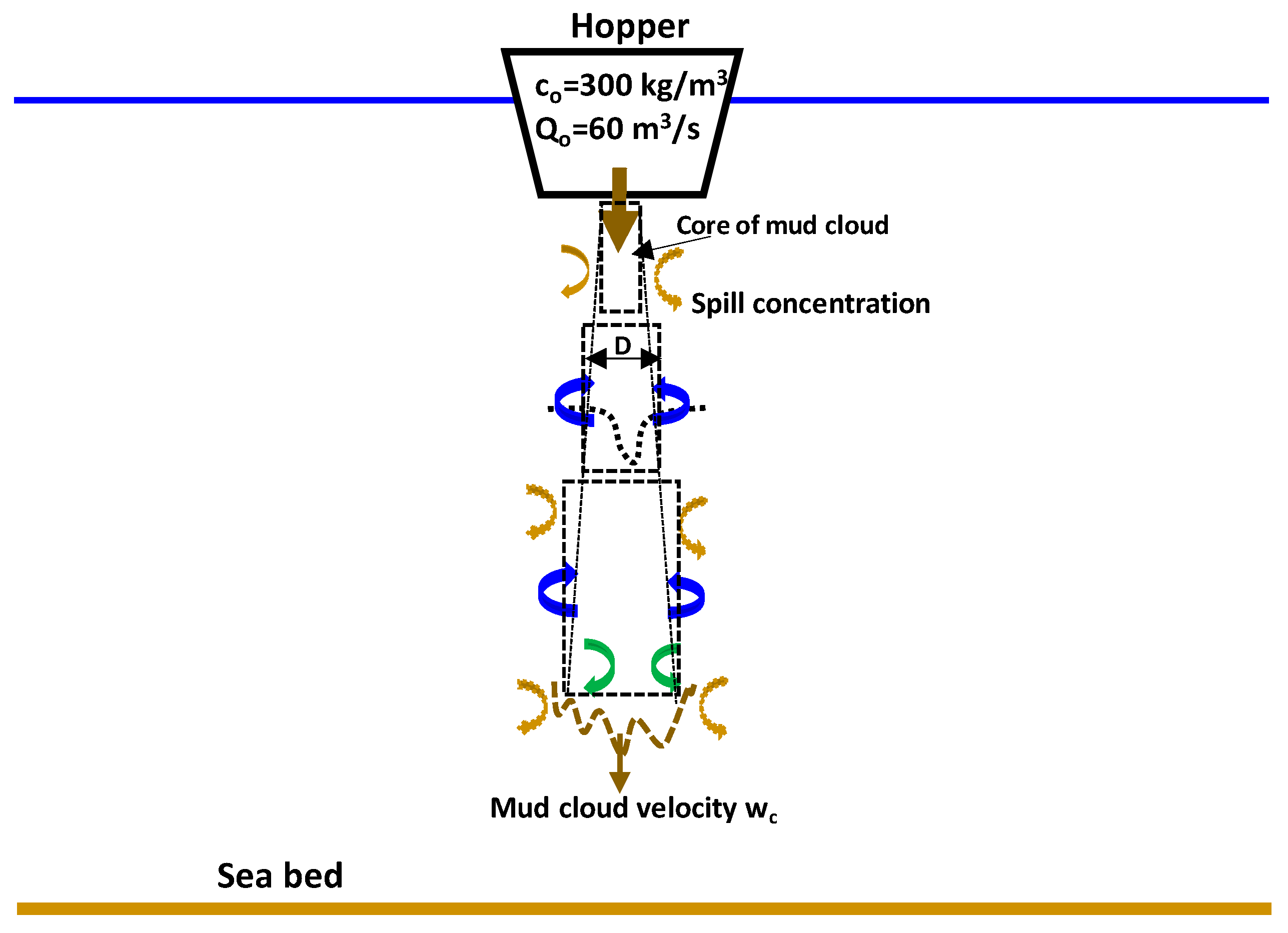
Figure 4.
Model results for calibration run, depth=15 m, Rochester site, USA.
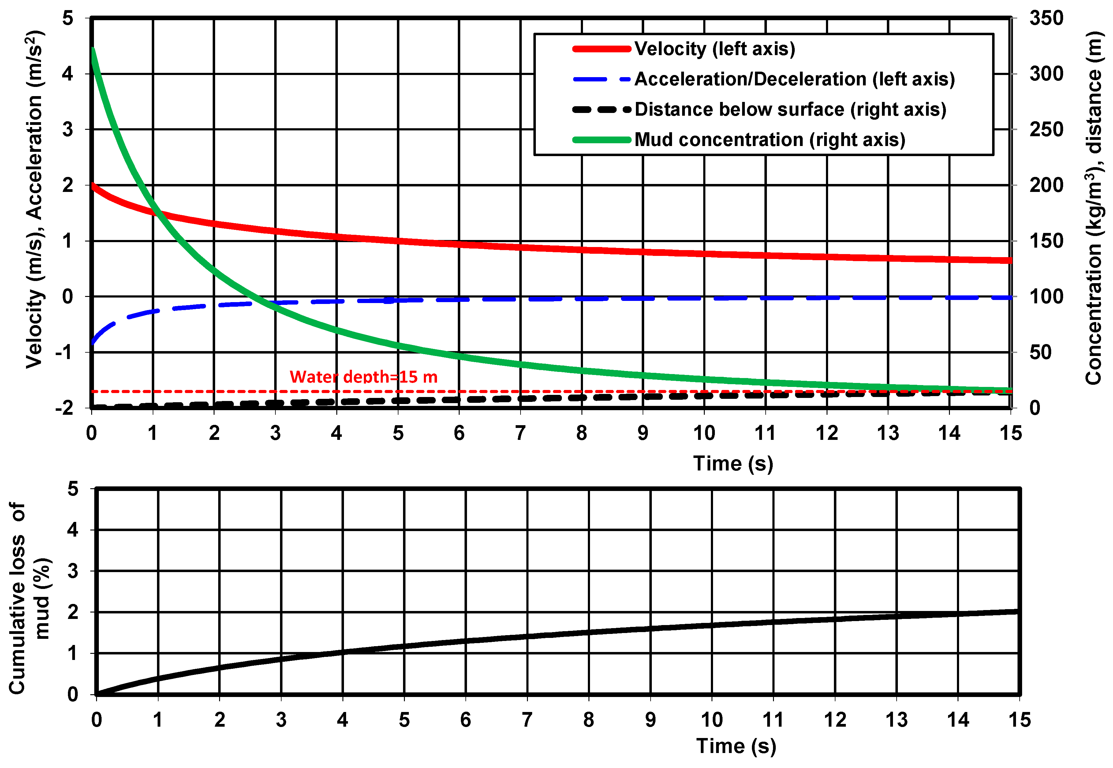
Figure 5.
Model results for depth=70 m.
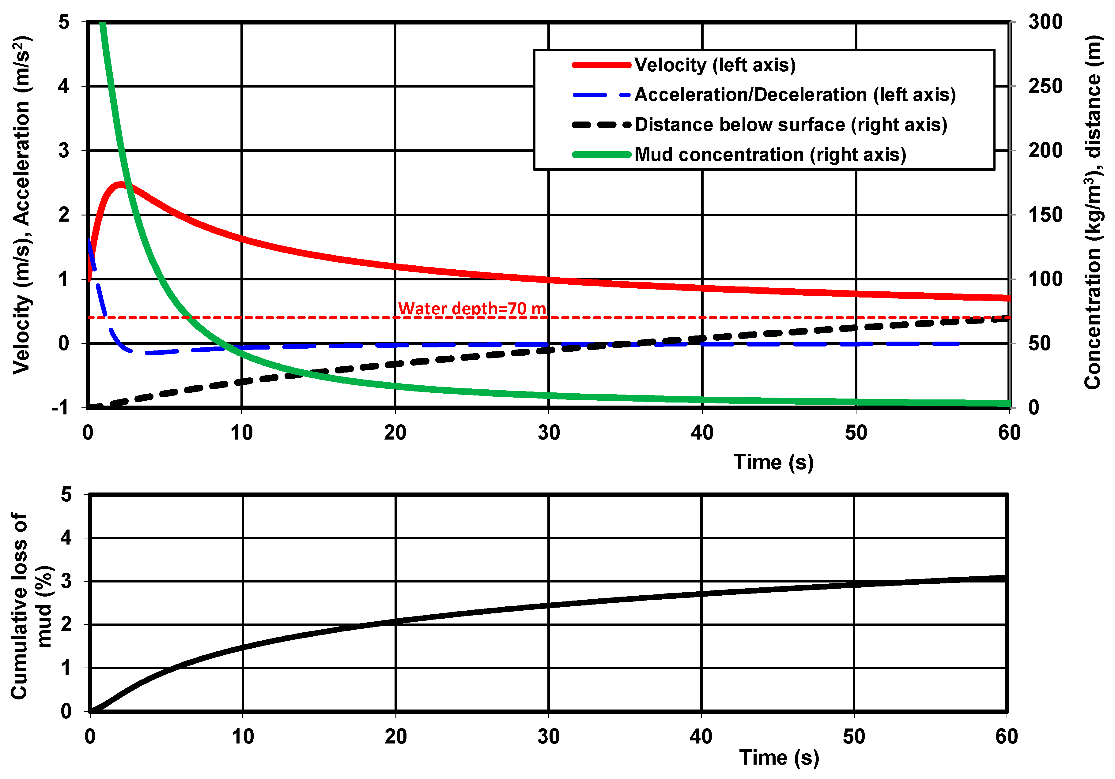
Figure 6.
Dispersion/diffusion of concentration as function of x (horizontal) and t.
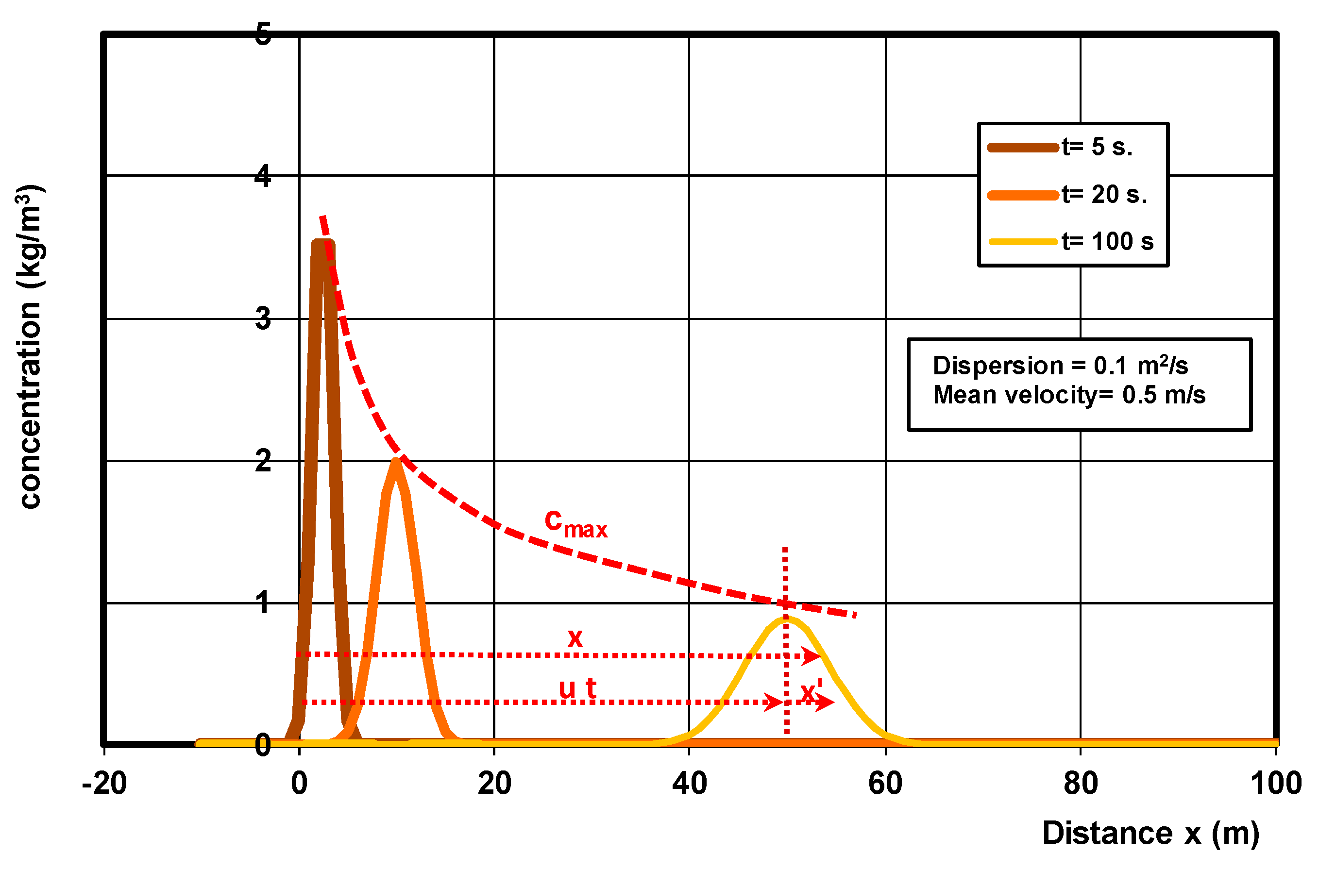
Figure 7.
Lateral mixing of dredging plume.
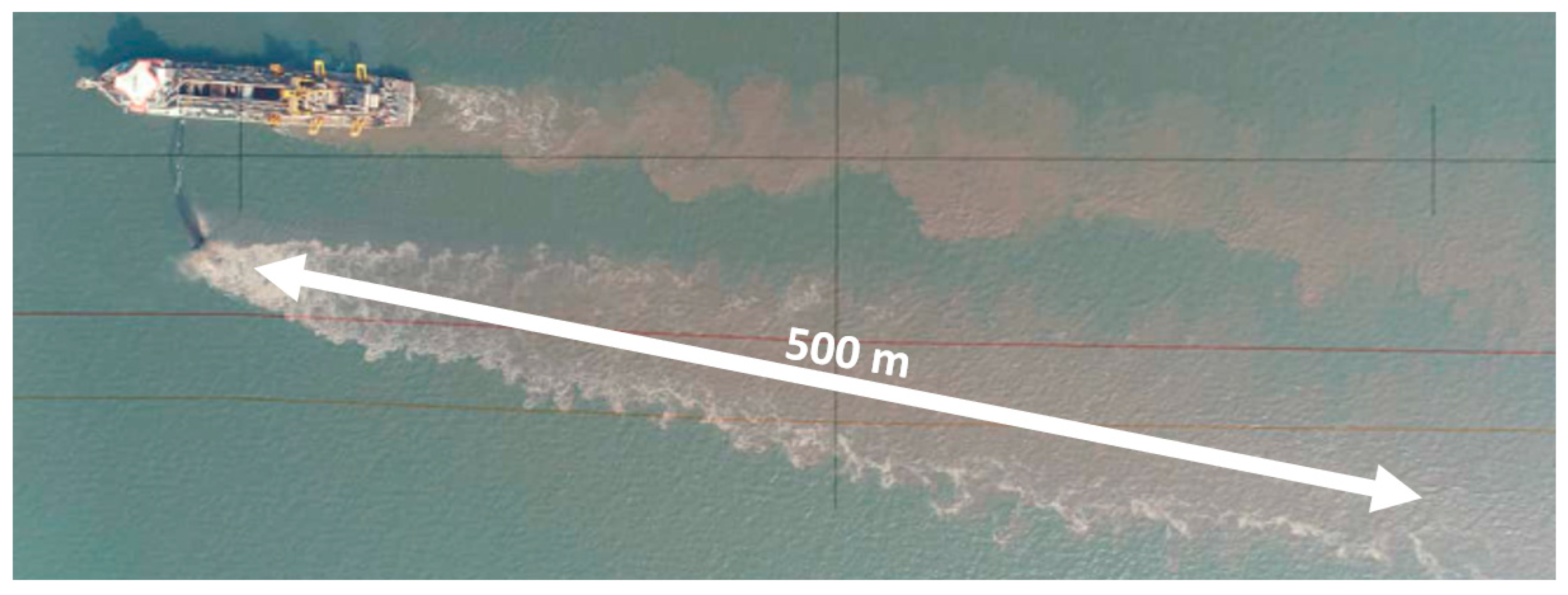
Figure 8.
Computed mud transport of SUSTIM2DV-model and SEDPLUME1D-model for overload conditions.
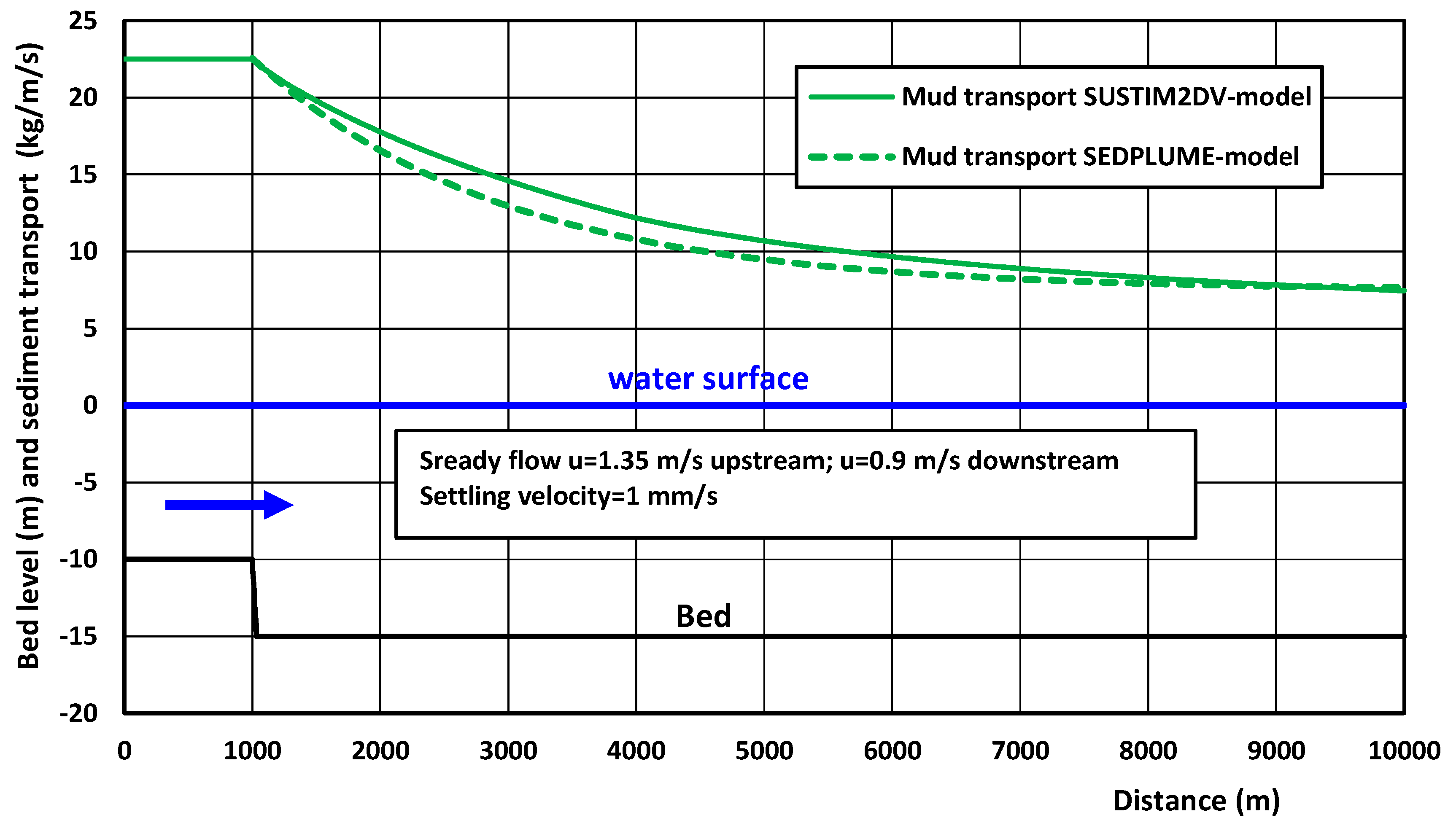
Figure 9.
Plan view of river with tunnel trench.
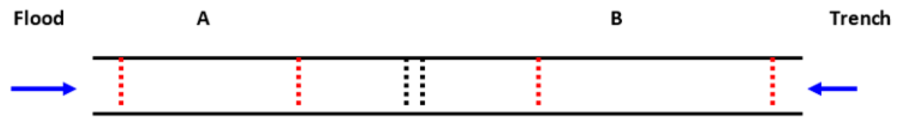
Figure 10.
Measured data in plume of dredger; simulation SEDPLUME1D h=10 m; u=0.5 m/s; β=0.6, bo=10 m co=100 mg/l, γ=0.3, ks=0.03 m, ws=0.5 mm/s (25 μm).
Figure 10.
Measured data in plume of dredger; simulation SEDPLUME1D h=10 m; u=0.5 m/s; β=0.6, bo=10 m co=100 mg/l, γ=0.3, ks=0.03 m, ws=0.5 mm/s (25 μm).
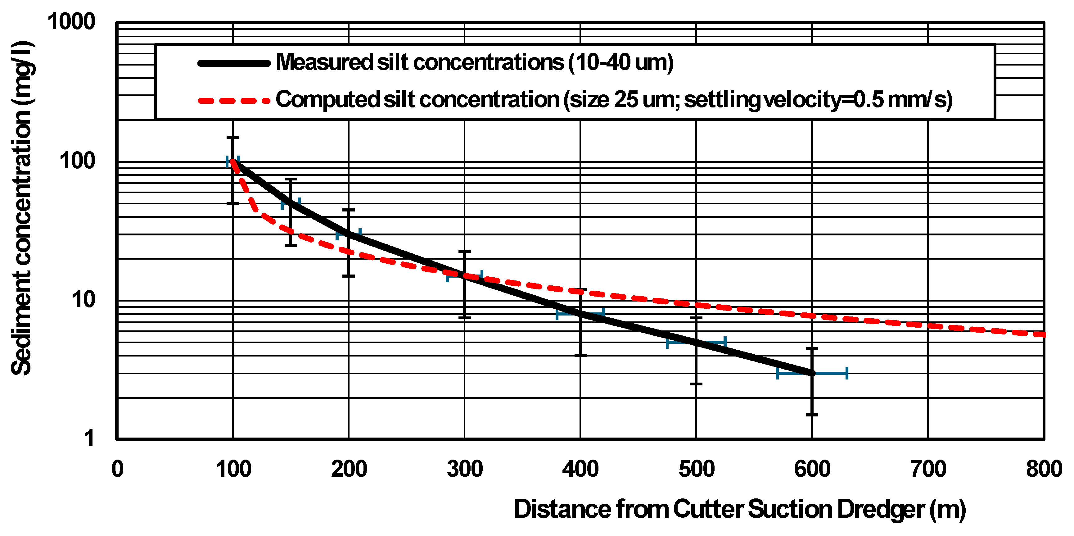
Figure 11.
Mud concentrations at source location in surface cell (upper) and in bottom cell (lower).
Figure 11.
Mud concentrations at source location in surface cell (upper) and in bottom cell (lower).

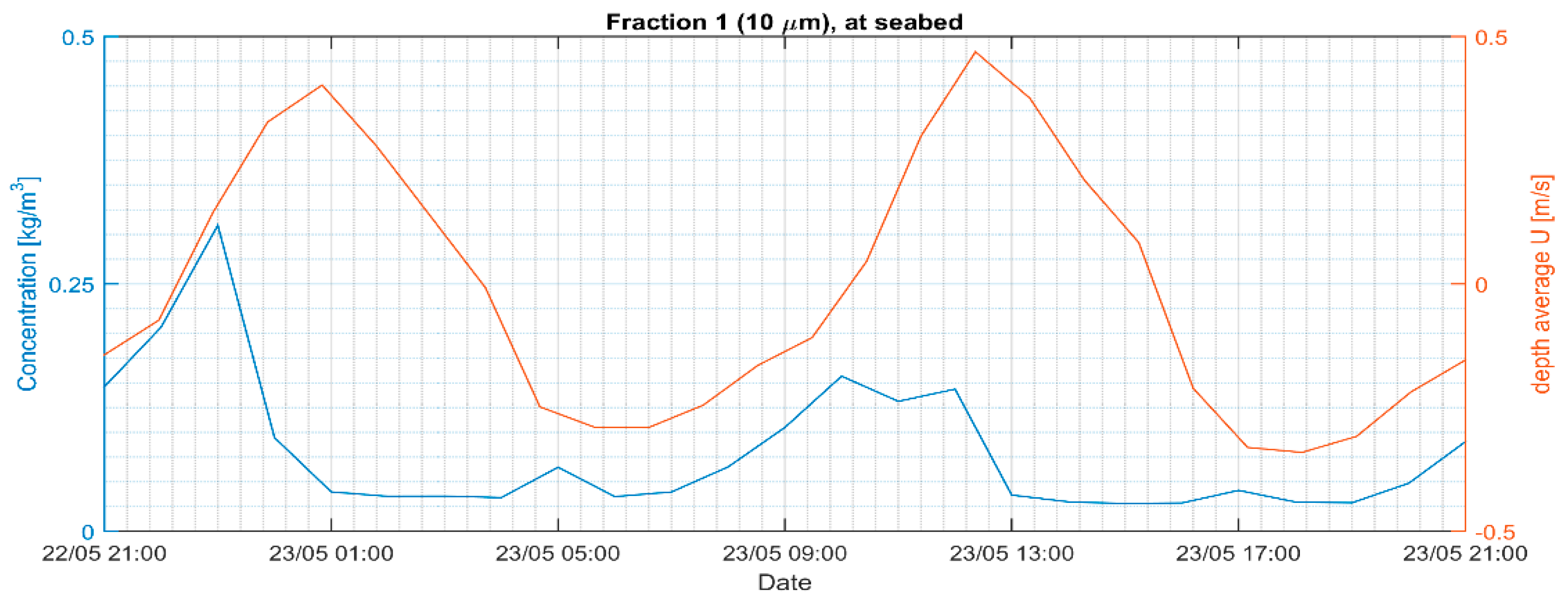
Figure 12.
Mud cloud of fraction 10 μm in bottom cell (mud source= red dot);.
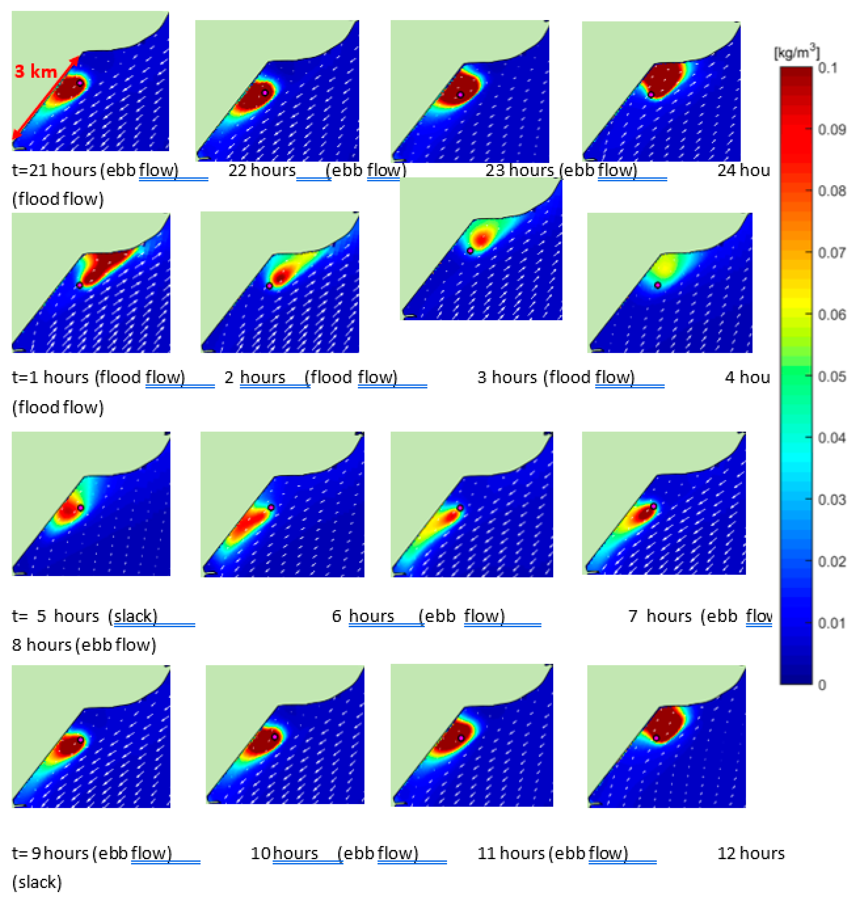
Figure 13.
Schematization of dispersion process in channel section with length Lch.
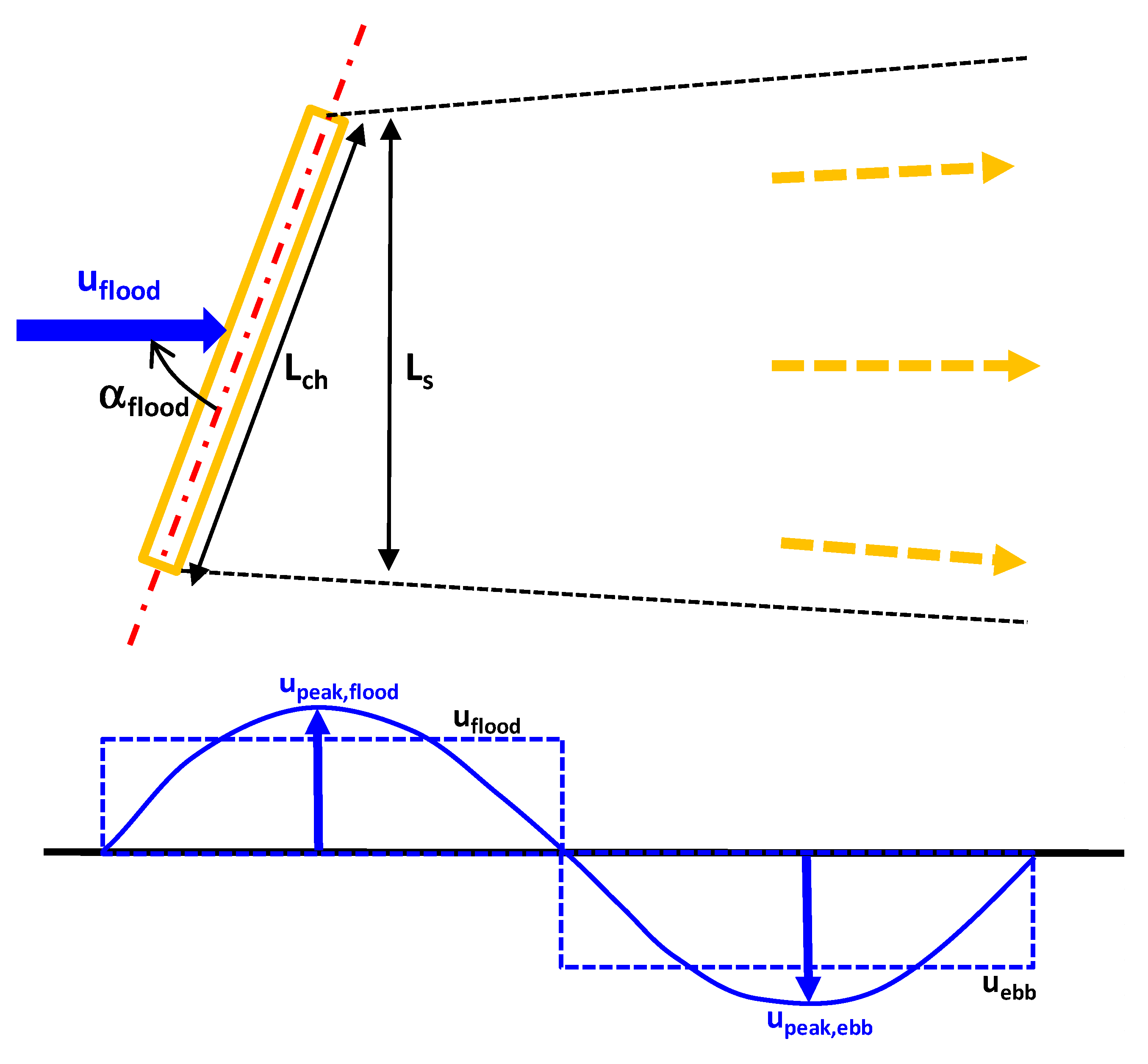
Figure 14.
Sediment concentrations as function of distance; SEDPLUME1D-model.
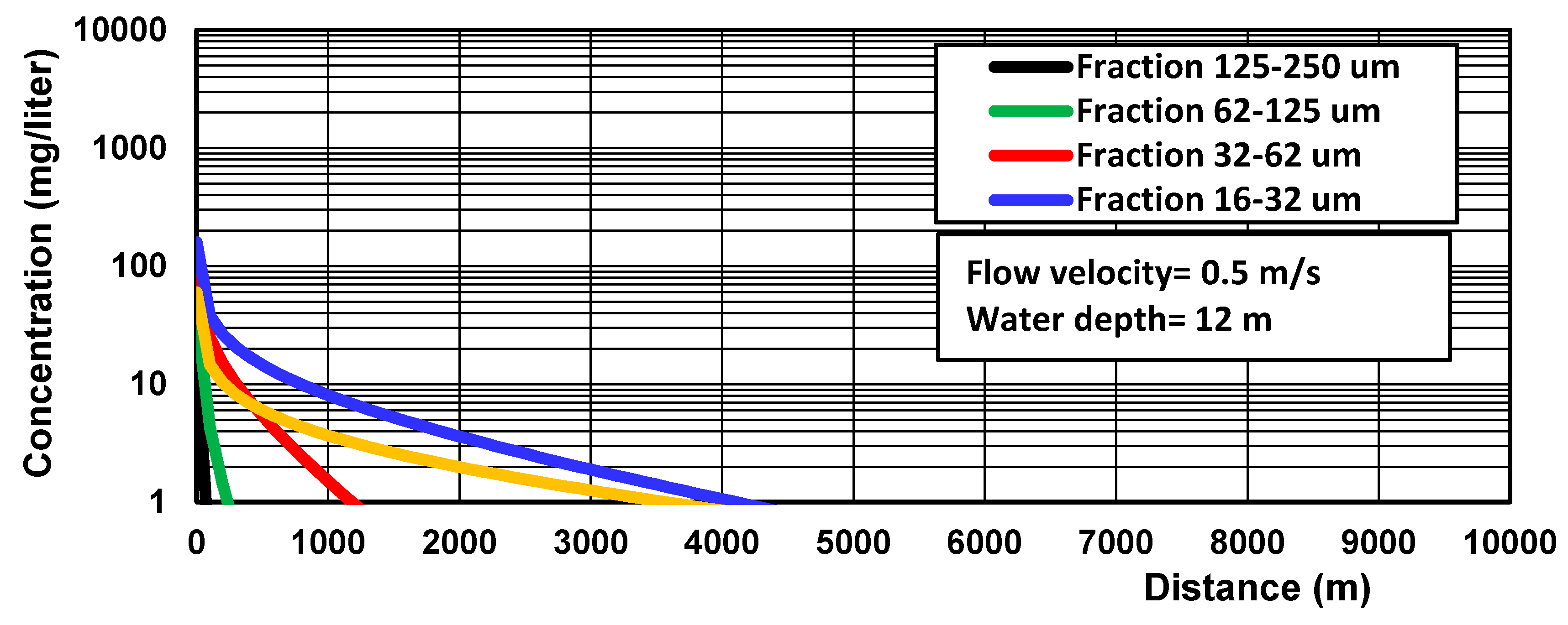
Figure 15.
Sediment layer thickness, deposition volume, plume width and plume area as function of distance.
Figure 15.
Sediment layer thickness, deposition volume, plume width and plume area as function of distance.
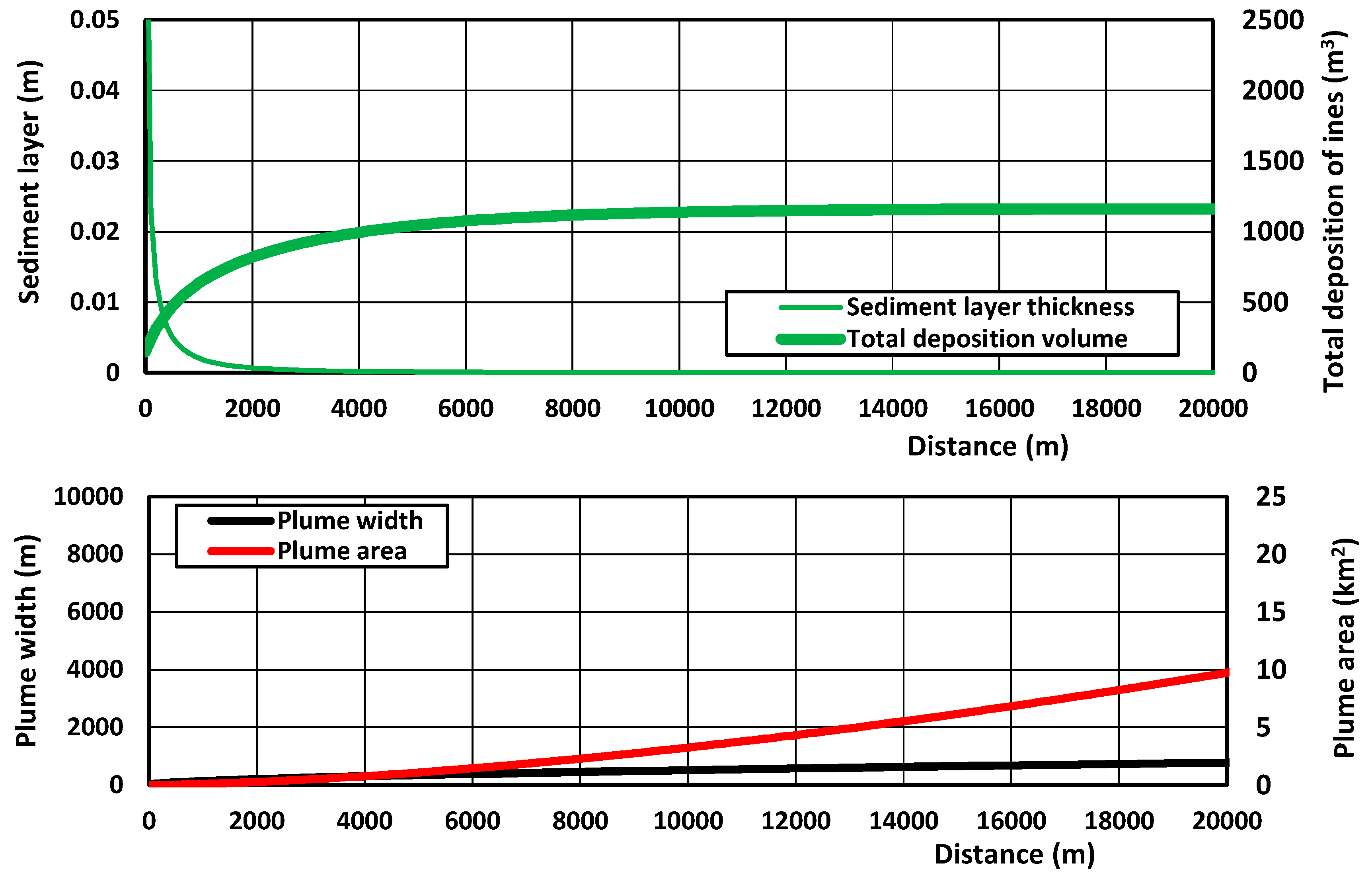

Table 1.
Sediment resuspension/loss parameter Sspill of dredging equipment.
| Dredging method | Production of dredged material (m3/hour) |
Background concentration Cbackground (mg/l) |
Increase of concentration ΔC at 50 m (mg/l) |
Decay time ΔTdecay after cessation dredging (hr) |
Spilling of fines Sspill (kg/m3) |
Spilling percentage Rspill (%) |
|---|---|---|---|---|---|---|
| Large suction hopper (maximum overflow) |
4000-6000 | 50-100 | 300-1000 | 1.5 | 20-50 | 5%-10% |
| Large suction hopper (limited overflow) |
4000-6000 | 50-100 | 200-400 | 1 | 10-20 | 2%-5% |
| Large suction hopper (no overflow) |
4000-6000 | 50-100 | 50-200 | 0.5-1 | 5-15 | 0.5-2% |
| Small suction hopper (limited overflow) |
1500-2500 | 20-50 | 50-200 | 0.5-1 | 5-15 | 0.5%-2% |
| Grab (open bucket) | 100-500 | 20-50 | 50-200 | 1 | 5-15 | 2%-5% |
| Grab (closed bucket) | 100-500 | 20-50 | 20-100 | 0.5-1 | 3-10 | 1%-2% |
| Bucket dredging | 300-600 | 20-50 | 50-200 | 0.5-1 | 5-15 | 2%-5% |
| Large cutter | >1000 | 20-50 | 50-200 | 0.5-1 | 5-15 | 2%-3% |
| Medium cutter | 200-1000 | 20-50 | 50-200 | 0.5-1 | 5-15 | 1%-2% |
| Small cutter | 100-200 | 20-50 | 20-100 | 0-0.5 | 3-10 | <1% |
| Hydraulic crane (various backhoes) |
100-200 | 20-50 | 100-500 | 1 | 5-50 | 2%-5% |
Table 2.
Dumping parameters of hopper dredgers.
| Parameter | Hopper 1 Alexander von Humboldt (Jan de Nul dredging) |
Hopper 2 Gateway (BosKalis dredging) |
|---|---|---|
| Hopper load volume (m3) | 9000 | 12000 |
| Hopper load area (m2) | 900 | 1200 |
| Number of double doors and area per door | 7 (4.1x8.2 m2) | 4 (4x5.4 m2) |
| Effective door area (m2) and relative door area (%) | 210 (23%) | 80 (7%) |
| Opening time of doors | 70 m2 after 60 s 140 m2 after 120 s 210 m2 after 180 s |
80 m2 after 60 s |
| Disposal time to release load (s) | 60 to 100 | 180 to 300 |
| Disposal discharge (m3/s) | 150 to 90 | 120 to 180 |
| Insertion speed of load through doors (m/s) | 2 to 1 | 1.25 to 0.85 |
Table 3.
Model calibration parameters for Rochester site, USA.
| Parameter | Measured value | Model value |
|---|---|---|
| Mud cloud density in hopper (kg/m3) Mud cloud concentration (kg/m3) |
1200 320 |
1200 (input) 320 (input) |
| Initial cloud diameter and height (m) | not measured | 2, 2 |
| Initial cloud velocity (m/s) | 2 | 2 (input) |
| Model parameters | - | cD=2, fw=0.05, a4=0.15; a5=0.001, Δt=0.1 s |
| Cloud diameter near bottom (m) | not measured | 4.5 |
| Mean cloud velocity near bottom (m/s) | 0.7 | 0.7 |
| Mean cloud concentration near bottom (kg/m3) | not measured | 15 |
| Overall sediment loss from cloud | <2% | 3% |
Table 4.
Dilution factors for a mud cloud (fines with settling velocity < 0.1 mm/s); M = 1 kg/m2 at t=0;.single release event at source location
Table 4.
Dilution factors for a mud cloud (fines with settling velocity < 0.1 mm/s); M = 1 kg/m2 at t=0;.single release event at source location
| Time (s) |
Distance (m) | Dilution factor | ||||
|---|---|---|---|---|---|---|
| Current= 0.5 m/s |
Current= 1 m/s |
1D case; longitudinal diffusion/mixing in main flow direction; no lateral mixing | ||||
| ε= 0.1 m2/s | 1 m2/s | 10 m2/s | 100 m2/s | |||
| 0.1 | c≅ 1 kg/m3 | ≅ 1 kg/m3 | ≅ 1 kg/m3 | ≅ 1 kg/m3 | ||
| 1 | 0.5 | 1 | c=0.9 | 0.3 | 0.09 | 0.03 |
| 10 | 5 | 10 | c=0.3 (γd≅1/3) | 0.09 (γd≅1/10) | 0.03 (γd≅1/30) | 0.01 (γd≅1/100) |
| 100 | 50 | 100 | c=0.09 (γd≅1/10) | 0.03 (γd≅1/30) | 0.009 (γd≅1/100) | 0.003 (γd≅1/300) |
| 1000 | 500 | 1000 | c=0.03 (γd≅1/30) | 0.01 (γd≅1/100) | 0.003 (γd≅1/300) | 0.001 (γd≅1/1000) |
| 10000 | 5000 | 10000 | c=0.01 (γd≅1/100) | 0.003 (γd≅1/300) | 0.0009 (γd≅1/1000) | 0.0003 γd≅1/3000) |
Table 5.
Dilution factors related to lateral mixing (bo=10 m).
| Distance from mud source location (m) | β= 0.5 | β= 0.7 |
|---|---|---|
| 200 | γd,lateral = 1/4 | γd,lateral = 1/9 |
| 500 | γd,lateral = 1/6 | γd,lateral = 1/15 |
| 1500 | γd,lateral = 1/10 | γd,lateral = 1/35 |
| 5000 | γd,lateral = 1/15 | γd,lateral = 1/80 |
| 10000 | γd,lateral = 1/20 | γd,lateral = 1/125 |
Table 6.
Concentration increase at tunnel trench location; SEDPLUME (γ=0.1; β=0.4).
| Initial mud concentrations | Mud concentration increase (mg/l) at trench location | |||
|---|---|---|---|---|
| Dump site A (flood) at 8.5 km |
Dump site B (flood) at 3 km |
|||
| SEDPLUME | DELFT3D | SEDPLUME | DELFT3D | |
| Fraction 32-63 μm; ws=2 mm/s; c1= 2250 mg/l | 1 | 1 | 15 | 15 |
| Fraction <16-32 μm; ws=0.4 m/s; c2= 1500 mg/l | 20 | 25 | 40 | 45 |
| Fraction < 16 μm; ws=0.1 m/s; c3= 1250 mg/l | 30 | 35 | 45 | 55 |
| Total: co=5000 mg/l | ≅50 mg/l | ≅60 mg/l | ≅105 mg/l | ≅120 mg/l |
Table 7.
Dilution factors fraction 10 μm (parallel to main flow) of SEDPLUME and DELFT3D-model.
|
Distance from mud source location (m) |
SEDPLUME β= 0.5 co= 2,000 mg/l; bo=10 m h=1.7 m; umean=0.3 m/s ws=0.075 mm/s (≅10 μm) |
SEDPLUME β= 0.7 co= 2,000 mg/l; bo=10 m h=1.7 m; umean=0.3 m/s ws= 0.075 mm/s (≅10 μm) |
DELFT3D-model co= 2,000 mg/l (depth and tide-averaged) |
| 750 | c= 210 mg/l (dilution 1/10) | c= 60 mg/l (dilution 1/35) | c= 100 mg/l (dilution 1/20) |
| 1500 | c= 100 mg/l (dilution 1/20) | c= 25 mg/l (dilution 1/40) | c= 40 mg/l (dilution 1/50) |
Disclaimer/Publisher’s Note: The statements, opinions and data contained in all publications are solely those of the individual author(s) and contributor(s) and not of MDPI and/or the editor(s). MDPI and/or the editor(s) disclaim responsibility for any injury to people or property resulting from any ideas, methods, instructions or products referred to in the content. |
© 2025 by the authors. Licensee MDPI, Basel, Switzerland. This article is an open access article distributed under the terms and conditions of the Creative Commons Attribution (CC BY) license (http://creativecommons.org/licenses/by/4.0/).
Copyright: This open access article is published under a Creative Commons CC BY 4.0 license, which permit the free download, distribution, and reuse, provided that the author and preprint are cited in any reuse.


