
Submitted:
12 May 2025
Posted:
13 May 2025
You are already at the latest version
Abstract
Background: Qualitative motion analysis revealed that the cervical spine moves according to a consistent pattern. This analysis calculates the relative rotation between vertebral segments to determine the sequence in which they contribute to extension, demonstrating high sensitivity and specificity. However, the extensive time required limits its applicability. This study investigated the feasibility of implementing a deep-learning model to analyze qualitative cervical motion. Methods: A U-Net architecture was implemented as 2D and 2D+t models. Dice similarity coefficient (DSC) and Intersection over Union (IoU) were used to assess the performance of the models. Intraclass Correlation Coefficient (ICC) was used to compare the relative rotation of individual vertebrae and segments to the ground truth. Results: IoU ranged from 0.37 to 0.74 and DSC ranged from 0.53 to 0.80. The ICC scores for relative rotation ranged from 0.62 to 0.96 for individual vertebrae and from 0.28 to 0.72 for vertebral segments. For segments, 2D+t models presented higher ICC scores compared to 2D models. Conclusion: This study showed the feasibility of implementing deep-learning models to analyze qualitative cervical motion in dynamic X-ray recordings. Future research should focus on improving model segmentation by enhancing recording contrast and applying post-processing methods.
Keywords:
Cervical spine
; qualitative motion analysis
; image segmentation
; U-net
; X-ray recording
; deep-learning model
; motion pattern
1. Introduction
A clear definition of physiological cervical spine motion is lacking. Segmental range of motion (sROM) has been proposed as a metric to evaluate cervical spine motion. However, sROM is limited by high intra- and interindividual variability and restricted to static endpoints [1,2]. Sequence of segmental contribution (SSC) is an alternative metric that analyses qualitative motion of the cervical spine [3]. In SSC relative rotations of the segments are tracked in dynamic X-ray recordings. The SSC is a consistent metric and has also been shown to have high sensitivity and specificity to detect motion patterns in individuals [4]. In a cross-validation study, two methods to analyze cervical spine motion in dynamic X-ray recordings demonstrated excellent agreement with a median difference below 0.2 degrees [5]. Motion pattern analysis revealed that various segments contribute at different moments during the extension movement of the cervical spine.
In young asymptomatic individuals, a consistent motion pattern of vertebrae C4 to C7 was found during the extension movement [4]. The pattern is defined as the order of maximum contribution of each motion segment to the extension movement, i.e., a peak in the relative rotation with respect to the cumulative amount of rotation of vertebrae C4 to C7. An RCT that compared anterior cervical discectomy with arthroplasty (ACDA) to anterior cervical discectomy with fusion (ACDF) reported that ACDA restored the consistent motion pattern one year after surgery [6,7]. However, after long-term follow-up, the motion pattern was absent in both treatment groups. The range of motion (ROM) was preserved in the long term in the ACDA group compared to ACDF group. In elderly subjects the ROM decreases over time due to the natural aging process. Qualitative analysis of cervical motion in elderly showed that the consistent motion pattern that was found in young asymptomatic individuals was absent [8]. The presence or absence of a consistent motion pattern among different groups raises questions and requires further investigation of cervical spine motion. In clinical practice, the presence of a consistent motion pattern, might play a role in clinical decision making.
Qualitative motion analysis has not been widely applied in research or clinical practice due to its time-consuming nature and the need for trained and experienced individuals. To increase feasibility, artificial intelligence (AI) algorithms are implemented to design deep learning models for the segmentation of cervical vertebrae. Promising results have been reported in studies that use these models to recognize cervical injuries on lateral X-rays, with accuracy for segmentation of cervical vertebrae ranging from 92 to 99% [9,10]. One study focused on calculating ROM of cervical vertebrae in static lateral flexion and extension radiographs and showed good accuracy [11].
In contrast to static X-rays, dynamic X-ray recordings can incorporate a temporal dimension, enabling a 2D+time (2D+t) model. This model can possibly better assess the relation of motion between the different frames of the recording. However, previous literature is inconclusive concerning an optimal model [12,13].
To enable qualitative analysis of the cervical spine, this study aims to develop a 2D and 2D+t deep learning model, trained on previously annotated dynamic X-ray recordings, to automatically calculate the relative rotation of each vertebra.
2. Materials and Methods
2.1. Population
Previous studies by our group investigated motion patterns in healthy, asymptomatic individuals in different age groups. Detailed information can be found in the published full-text articles [4,6,7,14,15]. Manually annotated data from these studies were combined for the training of this algorithm. Dynamic X-ray recordings were all made following the same protocol. Participants are seated on a crutch, adjustable in height, with their neck, shoulders, and head free. The subject is asked to move its head from maximal extension to maximal flexion, and vice versa, as fluent as possible and without moving the upper part of his body in about 10 seconds, using a metronome. While making the recordings the participants shoulders are kept as low as possible to ensure that all the cervical vertebrae are visible. The recordings were either made with the Siemens Arcadis Avantic VC10A, Toshiba Infinix Vi, or Philips Allura Xper FD20 X-ray system, capturing frames of 1024 × 1024 pixels at 15 frames per second. Images were not compressed.
2.2. Manual Annotation
Template areas containing each vertebral body and the skull base were manually drawn by two trained individuals (TB and VS) in the median frame of the recording, labeled C0-C7. The bottom part of the sella turcica and clivus are projected in the X-ray image as a stable and structure rich midline area of the skull. This is therefore an ideal template to track the movement of C0 (the skull base). Image recognition software, based on matching normalized gradient field images on a best-fit principle, was then used to locate the vertebrae in the other frames of the recordings [16]. The contours of the vertebra were manually checked and if necessary adjusted to fit the corresponding vertebrae in every frame of the recording (Figure A1, Appendix A). These image recognition-assisted manual annotations were considered the ground truth.
2.3. Development of the Model
Two image dimensions were evaluated to determine the best approach for analyzing motion patterns in clinical research. One dimension was centered around the cervical vertebrae in each frame and set to 640x640 pixels, maximizing the focus on the vertebrae while minimizing interference from other structures. The other dimension captured the entire extension or flexion movement of the cervical spine in a single view and was set to 832x576 pixels to assess the impact of including other structures.
2D models were compared to 2D+t models. The 2D+t models integrated temporal information with the hypothesis that the predicted vertebral shape will become more consistent over time, leading to more accurate relative rotation values. The neural network that was used for the segmentation task of this study was a five layered U-Net, widely used in medical segmentation studies [17,18]. For the 2D model, each frame was presented as input to the model. For the 2D+t model, multiple frames were presented as input to the model. All models have nine output channels, one for each of the eight vertebrae and one for the background class. To determine the ideal number of frames for the 2D+t models, an ablation study was performed. As pre-processing step, both image sizes were normalized with the mean and standard deviation of pixel values of the training subset. On the training dataset, data augmentation was applied to artificially increase the diversity of the training data by applying various transformations. Specifically, Gaussian noise was introduced and the contrast was adjusted. For both 2D and 2D+t models, the two dimensions were analyzed, resulting in four different models, models A to D. An overview of models A to D can be found in Table 1.
The output of the model, given in probability values, was transformed into a binary mask by applying a threshold between 0.1 and 0.9 (Figure A2, Appendix A). The optimal threshold for each vertebra was determined via the Precision-Recall (PR) curve, which focuses on foreground pixel performance. The threshold varied between vertebrae per model (Table A1, Appendix A).
2.4. Dataset
Dynamic X-ray recordings with annotated and corrected contours were available for 39 healthy controls. Extension recordings were made at two time points, resulting in 78 extension recordings. In eleven cases flexion recordings were also analyzed, resulting in a total of 89 recordings in these 39 subjects. Each recording consisted of ±52 individual frames that were analyzed. Altogether this resulted in a total of 4671 frames. The recordings were split into subsets for training, validation, and testing, with a split of approximately 55-20-25%, respectively (Table 2). Resulting in 2709 frames for training, 964 frames for validation, and 998 frames for testing. Recordings were allocated per individual into one of the subsets. The learning rate for all models was set to 0.0001, with a maximum of 300 epochs.
2.5. Mean Shape
The model predictions were made per individual frame of a recording, resulting in a slightly different shape in each frame, which could be caused by over-projection of the 3D structures in the 2D plane or due to coupled motion. However, vertebrae are rigid bodies, thus their actual shape does not vary throughout the movement. To include this physical property, a mean shape was created for each vertebra per recording to calculate the relative rotation.
To quantify the overlap between the mean shape and the ground truth, the Intersection over Union (IoU) was calculated. Similarly, the IoU was calculated between the mean shape and the model predictions.
2.6. Outcome Measures
To assess the performance of each model, the IoU and the Dice similarity coefficient (DSC) were calculated.
The IoU measures the overlap between the predicted segmentation and the ground truth by calculating the ratio of the intersection area to the union area (Equation (1)). Typically, IoU values above 0.7 are deemed good, those between 0.5 and 0.7 indicate moderate overlap, and values below 0.5 suggest poor overlap
IoU (A,B)=(|A∩B|)/(|A∪B|),
The DSC is also a measure of overlap between the predicted segmentation and the ground truth, by dividing twice the size of the intersection area with the sum of their individual sizes (Equation (2)) [19]. A DSC is considered good when above 0.7, a DSC between 0.5 and 0.7 is considered moderate and below 0.5 is considered poor [20]. The main difference between IoU and DSC is the fact that under- and over-segmentation is penalized more by the IoU.
DSC (A,B)=(2×|A∩B|)/(|A|+|B|),
The primary outcome will be the intraclass correlation coefficient (ICC) of the relative rotation of individual vertebrae over time. The relative rotation values will be calculated using a mean shape of each vertebra per recording. The mean shape was positioned on the centroid of the model prediction on each frame, and subsequently rotated iteratively until maximal overlap was achieved. The fitted mean shape was used to calculate the rotation of each vertebra in the consecutive frames of the entire recording (dθC), as shown in Equation (3), where θ denotes an angle in frame t.
dθC= θC(t) – θC(t-1),
The first frame of the recording dθC = 0 as there was no preceding frame (t − 1). For the 2D+t models, dθC = 0 for frames that were not considered as a middle frame, such as the first and last frames of the recording in case of three input frames. With C indicating one of the eight vertebrae.
Secondary outcome measure was the ICC of the relative rotation of vertebral segments over time. Relative rotation for segments was also calculated using a mean shape. With the relative rotation values of each vertebra, the relative rotation between two vertebrae (dθR) was calculated via Equation (4).
dθR= dθCk – dθCl,
With Ck and Cl each indicating another vertebra.
The Wilcoxon Signed Rank test was used to assess significant differences in outcome performance between the different models. A p-value ≤0.05 was considered statistically significant.
3. Results
3.1. Ablation Study 2D+t
The ablation study of the 2D+t models was conducted using three, five, seven, and nine input frames. For both model configurations, seven input frames most frequently resulted in the significantly highest score. Results of the ablation study for Model C and Model D can be found in Appendix A, Table A2 and Table A3.
3.2. Model Performance
The mean IoU score ranged from 0.37 to 0.72 for model A, from 0.51 to 0.72 for model B, from 0.45 to 0.74 for model C, and from 0.49 to 0.72 for model D. The mean DSC ranged from 0.53 to 0.82 for model A, from 0.66 to 0.82 for model B, from 0.61 to 0.83 for model C, and from 0.64 to 0.82 for model D. The mean IoU and DSC for each vertebra across all models are presented in Table 3, with the highest score indicated in bold. An asterisk denotes a significant difference between the highest score and the scores from the other three models.
Figure 1 illustrates the segmentation of each vertebra created by model C comparing the first, median, and final frames of the recording to the ground truth. From top to bottom, good, average, and poor model segmentation results are displayed compared to the ground truth. Equal results were observed for models A, B, and D, as seen in Figure A3, Figure A4 and Figure A5, Appendix A.
3.3. Mean Shape
The mean shape was generated for vertebrae C1-C7 for each model option, excluding the skull base C0 because of its variable shape. For several recordings per model, it was not possible to create a mean shape due to deviations in the model segmentation. Figure 2 displays the mean shape of C5 compared to the ground truth and the model segmentation. The mean shape that was generated for the other vertebrae can be seen in Figure A6 and Figure A7, Appendix A.
To compare the accuracy of the mean shape generated by the model to the ground truth, the IoU was calculated for each vertebra and model, presented in Table 4. The IoU score ranged from 0.56 to 0.80 for model A, from 0.56 to 0.84 for model B, from 0.61 to 0.84 for model C, and from 0.61 to 0.84 for model D.
3.4. ICC of Relative Rotation of Individual Vertebrae
The ICC score for individual vertebrae ranged from 0.819 to 0.962 for model A, from 0.798 to 0.948 for model B, from 0.683 to 0.907 for model C, and from 0.620 to 0.878 for model D, presented in Table 5. The highest mean score between the models is indicated in red bold. The number of recordings on which the ICC is based is also presented in Table 5. Figure 3a illustrates the trajectory of C1 Model A with a high ICC (0.990), and Figure 3b illustrates the trajectory of C3 Model D with a low ICC (0.298).
3.5. ICC of Relative Rotation of Vertebral Segments
The ICC score for vertebral segments ranged from 0.511 to 0.685 for model A, from 0.408 to 0.627 for model B, from 0.382 to 0.770 for model C, and from 0.281 to 0.724 for model D, presented in Table 6. The highest mean score between the models is indicated in red bold. The number of recordings on which the ICC is based is also presented in Table 6. Figure 4a illustrates the trajectory of C1-C2 Model D with a high ICC (0.890), and Figure 4b illustrates the trajectory of C5-C6 Model B with a low ICC (0.000).
4. Discussion
The results of this study show the feasibility of implementing a 2D and 2D+t deep learning model to recognize cervical vertebrae in dynamic X-ray recordings. Moreover, based on acceptable ICC scores for relative rotation of individual vertebrae, the investigated models can accurately track vertebrae over time. To calculate the segmental relative rotation, the models need to be further improved, as these results are poor to moderate.
In the ablation study for the 2D+t models, an improvement in the IoU score was observed when seven frames were compared to three or five frames. In current literature, three or five frames are often used in static imaging [12,21,22]. A model containing a time dimension might benefit from more information because we analyze motion of the cervical spine, where motion can be observed between frames. However, using nine frames did not lead to further improvement in IoU score, indicating that too much information away from the median frame leads to a worse outcome.
The IoU results of the different models are overall better for C1 to C3 compared to C0 and C4 to C7. Figure 1 and Figure A3-A5 also display that the lower vertebrae are more fragmented. This can be explained by the different features of the cervical vertebrae. C4 to C6 have a more similar shape, with long spinous processes and shorter distance in between, and are therefore, more difficult to distinguish from each other [23]. Overprojection of the shoulders can challenge the model in accurate recognition and differentiation of the lower vertebrae, especially C7. This is also true for human observers. C0 is difficult to recognize because in several recordings C0 is not completely visualized, so the contour of the part that is visible varies even more, as illustrated in Figure 1 and Figure A3, Figure A4 and Figure A5.
Inaccuracies in model segmentation can partially be explained by the quality of recordings. In multiple recordings the contrast between the vertebrae and background is less pronounced, which leads to worse outcomes. In contrast, recordings with distinct edges of the vertebrae and enhanced contrast lead to improved outcomes. In some included recordings, increased tube voltage was necessary to enhance visualization of vertebrae C6 and C7 located behind the shoulders, albeit at the expense of overexposure to the other structures, resulting in light grey vertebrae with minimal contrast against the background. These findings provide valuable knowledge for the acquisition of future X-ray recordings. Examples of recordings with low and good results are presented in Figure A8 and Figure A9, Appendix A.
Even though the shape of vertebral bodies is rigid, the model segmentation shows different shapes of the vertebral bodies over time. This variance in segmentation is caused by overprojection of structures on the recording. The generated mean shape for all vertebrae had an acceptable IoU compared to the ground truth, presented in Table 4. Similarly to the model segmentation, C5 to C7 demonstrated lower IoU scores. This emphasizes the complexity for the model to accurately segment the lower vertebrae. The proposed solution for the different shapes, creating a mean shape, led to better results for the ICC scores, presented in Table 6 and Table A4.
The ICC scores for relative rotation of individual vertebrae are similar between the 2D and 2D+t models. The mean ICC scores ranged from good to excellent, indicating that all models can accurately track individual vertebrae over time. The ICC scores for relative rotation of vertebral segments are lower. This can be explained by comparing the overall rotation of an individual vertebra to a segment. Boselie et al. calculated that between frames a segment can rotate as little as 0.3 degrees, less than the measurement error [4]. Rotation of individual vertebrae between frames ranges from 2 to 3.5 degrees, illustrated in Figure 3a,b. Therefore, rotation over time of individual vertebrae is less sensitive to measurement errors or segmentation inaccuracies. Additionally, inaccuracies in segmentation of vertebrae above or below do not affect the measured relative rotation of the individual vertebra.
When the 2D and 2D+t models are compared to track vertebral segments over time, the 2D+t results in higher ICC values, confirming that incorporating a time dimension, will lead to a more consistent segmentation shape than the 2D models. We also analyzed two image sizes to measure if a more centralized frame led to more accurate model segmentation. Between the image sizes, we did not observe a relevant difference in our outcomes, indicating that both can be used for qualitative cervical motion analysis.
A limitation of this study is the angular shape of the ground truth segmentation, as the natural shape of a vertebra is smoother. The ground truth is created with the algorithm of Reinartz et al., which is already very time consuming [16]. Adding a greater number of points to achieve a smoother and more realistic shape would further extend the processing time. The difference in shape can lead to lower IoU or DSC scores. It is favorable that the model segmentation already creates a more natural looking vertebra.
Another limitation is that the 2D recordings only capture the sagittal rotation. Other rotation planes, e.g. axial, lateroflexion or coronal, have not been analyzed.
Lastly, the number of recordings included in ICC calculation is limited. Some ICC values are based on one or two recordings. Therefore, these values should be interpreted with caution. For each level, the recording was excluded if the mean ICC was negative or if the recording contained at least one outlier. A negative value occurs when the ground truth segmentation moves opposite to the model segmentation. An outlier occurs when the threshold, based on the minimum and maximum raw values of the gold standard, is exceeded. The most probable cause of an outlier is the model segmentation used to fit either the mean shape or the model segmentation in the subsequent frame. Deviating shapes and differences in shape between consecutive frames can result in sub-optimal fits during rotation. Also, most outliers were detected for C5 and C6. The shape of these vertebrae is very similar, making it more complex for the model to differentiate between C5 and C6. We decided to exclude these recordings because the outliers originate from model segmentation issues.
For future use, we would like to improve the model segmentation, which will lead to less outliers. Model segmentation can be improved by several methods. One method is improving the quality of the recordings by enhancing the contrast. This can be achieved by histogram equalization or histogram matching [24]. Another method is training the model to recognize the vertebra in a specific sequence. Incorporating a sequence will prevent the model from interchanging vertebrae. Also, post-processing techniques can be applied when the model segmentation is fragmented. Currently, only the largest segment is selected for further analysis in the mean shape and relative rotation calculations. By incorporating post-processing methods, fragmented segments can be merged into a single segmentation using techniques like morphological operations, e.g. dilation and closing, and majority voting for consistent foreground pixels across multiple frames [25]. Another method is to recognize frames that cause outliers and replace these frames with the preceding or following frame. This is especially relevant for recordings with a limited number of outliers. Improving the model segmentation in each frame with post-processing techniques will result in a more accurate mean shape and more precise relative rotation values, ultimately improving the ICC scores. With improved segmentation, the model can be used for measuring other metrics, such as the cervical lordosis and T1 slope. Analyzing these metrics has already been shown to be feasible in static X-rays [26]. Analyzing these metrics in recordings will provide further insights into the normal movement of the cervical spine.
This model can accurately calculate the relative rotation of an individual vertebra. However, the relative rotation analysis of vertebral segments needs to be further improved to enable motion pattern analysis. If different motion patterns can be distinguished, the next step can be to differentiate between normal and pathological patterns. The final step would be for the motion pattern to serve as an aid in clinical decision-making. The current model is trained on healthy subjects. To recognize deviating shapes caused by disease, trauma, or surgical interventions, the model will need additional training and validation with these shapes.
5. Conclusions
Implementing a 2D or 2D+t deep learning model to analyze the relative rotation of individual vertebrae leads to accurate results compared to the ground truth. For the calculation of the relative rotations of vertebral segments, the 2D+t models, incorporating a temporal dimension, seem to do better than 2D models. However, these results remain poor and require further improvement. Future research should focus on improving the model segmentation by enhancing contrast and applying post-processing methods. This will enable analyses of motion patterns in large groups.
Author Contributions
Conceptualization, E.v.S., V.S., H.v.S, and T.B.; methodology, E.v.S., V.S., E.C., and T.B.; software, V.S., E.C., and T.B.; validation, E.C..; formal analysis, E.v.S., V.S., E.C. and, T.B..; investigation, E.v.S. and E.C.; resources, V.S. and T.B.; data curation, E.v.S., V.S. and, E.C.; writing—original draft preparation, E.v.S., V.S. and, E.C; writing—review and editing, M.B., A.S., H.v.S. and, T.B.; visualization, E.v.S., V.S., E.C., and T.B.; supervision, M.B., A.S., H.v.S. and, T.B.; project administration, E.v.S. and E.C.; funding acquisition, n.a. All authors have read and agreed to the published version of the manuscript.
Funding
This research received no external funding.
Conflicts of Interest
The authors declare no conflicts of interest.
Abbreviations
The following abbreviations are used in this manuscript:
| 2D | Two dimensional |
| 2D+t | Two dimensional + time |
| AI | Artificial intelligence |
| DSC | Dice similarity coefficient |
| ICC | Intraclass Correlation Coefficient |
| IoU | Intersection over Union |
| ROM | Range of motion |
| sROM | Segmental range of motion |
| SSC | Sequence of segmental contribution |
Appendix A
Figure A1.
Manual annotations on a median frame.
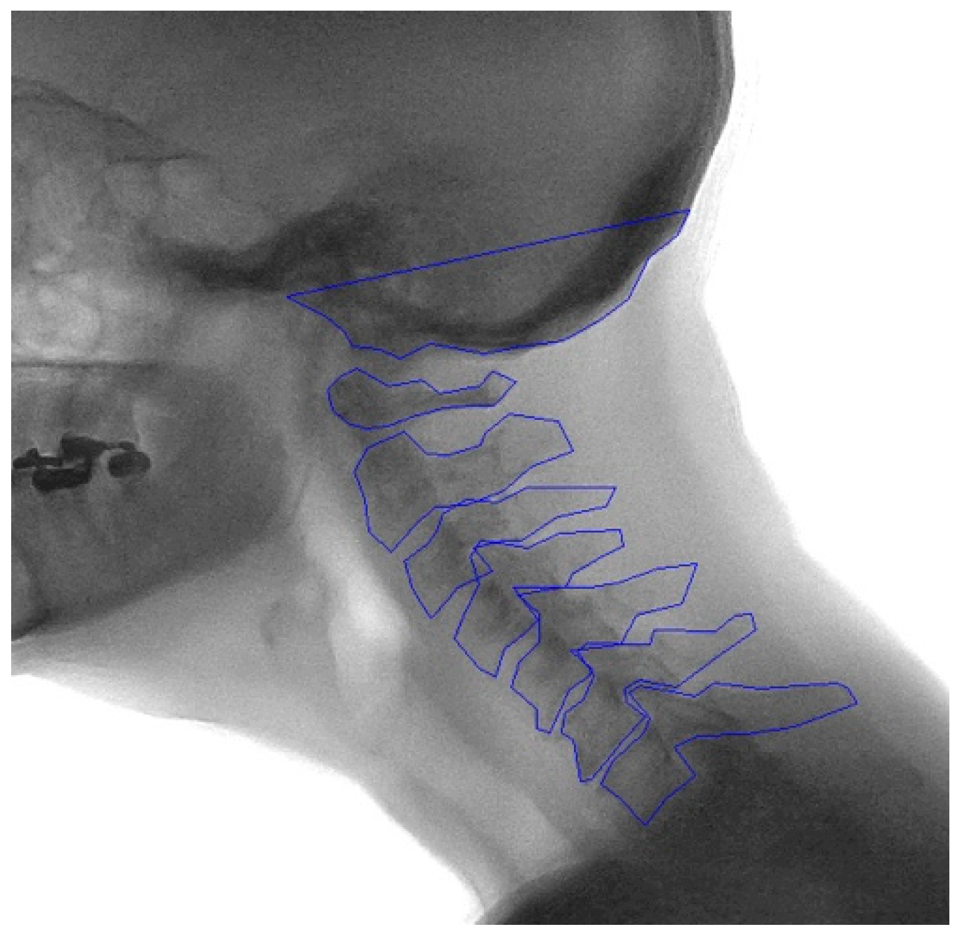
Figure A2.
Binary mask.


Table A1.
Optimal threshold per vertebra of models A to D.
| Channel | A | B | C | D |
|---|---|---|---|---|
| C0 | 0.7 | 0.8 | 0.9 | 0.4 |
| C1 | 0.1 | 0.1 | 0.1 | 0.6 |
| C2 | 0.9 | 0.9 | 0.5 | 0.9 |
| C3 | 0.1 | 0.1 | 0.7 | 0.7 |
| C4 | 0.1 | 0.1 | 0.3 | 0.1 |
| C5 | 0.1 | 0.1 | 0.1 | 0.1 |
| C6 | 0.1 | 0.1 | 0.1 | 0.1 |
| C7 | 0.1 | 0.1 | 0.1 | 0.1 |
| Background | 0.1 | 0.9 | 0.1 | 0.1 |
Table A2.
Ablation study model C: IoU and DSC per vertebra for the varying number of input frames.
| IoU | DSC | |||||||
|---|---|---|---|---|---|---|---|---|
| Frames | 3 | 5 | 7 | 9 | 3 | 5 | 7 | 9 |
| C0 | 0.45 | 0.50* | 0.45 | 0.44 | 0.61 | 0.65* | 0.61 | 0.61 |
| C1 | 0.68 | 0.69 | 0.72* | 0.69 | 0.79 | 0.8 | 0.82* | 0.8 |
| C2 | 0.49 | 0.72 | 0.72 | 0.73* | 0.65 | 0.82 | 0.82 | 0.82* |
| C3 | 0.72 | 0.73 | 0.74* | 0.7 | 0.82 | 0.82 | 0.83 | 0.8 |
| C4 | 0.59 | 0.62 | 0.63 | 0.6 | 0.72 | 0.74 | 0.74 | 0.71 |
| C5 | 0.47 | 0.5 | 0.52* | 0.49 | 0.61 | 0.64 | 0.64* | 0.62 |
| C6 | 0.5 | 0.52 | 0.57* | 0.54 | 0.63 | 0.65 | 0.7* | 0.67 |
| C7 | 0.49 | 0.5 | 0.55* | 0.51 | 0.64 | 0.64 | 0.68* | 0.65 |
IoU= Intersection over Union, DSC= Disc Similarity Coefficient. The highest IoU and DSC values for each vertebra are indicated in bold. Significant differences compared to all other options are marked with an asterisk.
Table A3.
Ablation study model D: IoU and DSC per vertebra for the varying number of input frames.
| IoU | DSC | |||||||
|---|---|---|---|---|---|---|---|---|
| Frames | 3 | 5 | 7 | 9 | 3 | 5 | 7 | 9 |
| C0 | 0.48 | 0.48 | 0.49 | 0.46 | 0.63 | 0.63 | 0.64 | 0.62 |
| C1 | 0.68 | 0.71* | 0.7 | 0.69 | 0.78 | 0.81 | 0.81 | 0.79 |
| C2 | 0.71 | 0.71 | 0.72 | 0.72* | 0.81 | 0.81 | 0.82 | 0.82* |
| C3 | 0.71 | 0.69 | 0.72* | 0.69 | 0.81 | 0.8 | 0.82* | 0.8 |
| C4 | 0.62 | 0.57 | 0.63 | 0.6 | 0.74 | 0.71 | 0.75 | 0.72 |
| C5 | 0.57 | 0.49 | 0.58 | 0.5 | 0.7 | 0.64 | 0.71* | 0.64 |
| C6 | 0.59 | 0.52 | 0.59 | 0.53 | 0.72 | 0.66 | 0.73 | 0.66 |
| C7 | 0.55* | 0.52 | 0.54 | 0.46 | 0.68* | 0.66 | 0.67 | 0.6 |
IoU= Intersection over Union, DSC= Disc Similarity Coefficient. The highest IoU and DSC values for each vertebra are indicated in bold. Significant differences compared to all other options are marked with an asterisk.
Figure A3.
Comparison between the ground truth and the segmentation made by model A. Each vertebra is indicated with another color. From left to right: first-median-last frame of the recording. From top to bottom, the comparison with the best visual comparison to the worst visual comparison.
Figure A3.
Comparison between the ground truth and the segmentation made by model A. Each vertebra is indicated with another color. From left to right: first-median-last frame of the recording. From top to bottom, the comparison with the best visual comparison to the worst visual comparison.
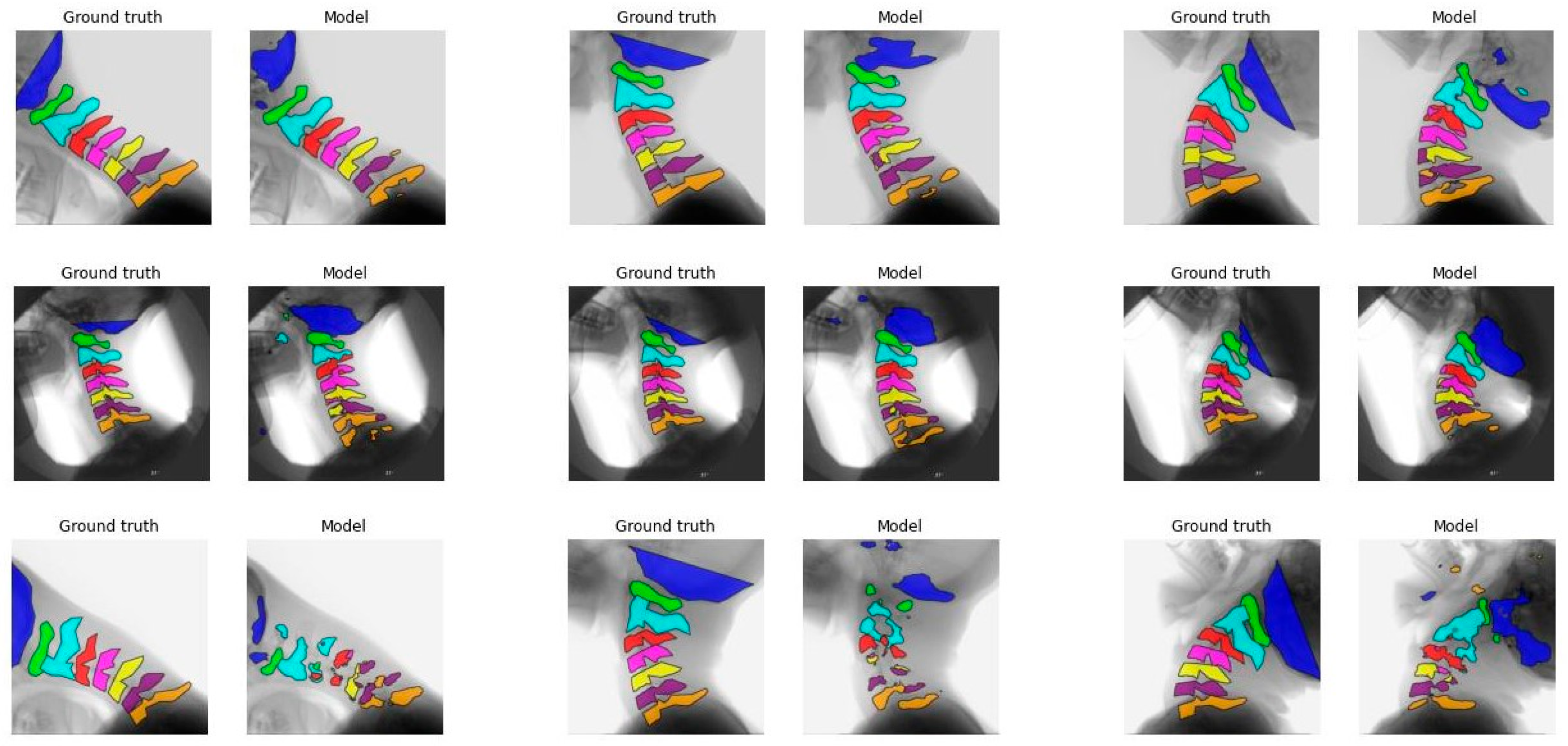
Figure A4.
Comparison between the ground truth and the segmentation made by model B. Each vertebra is indicated with another color. From left to right: first-median-last frame of the recording. From top to bottom, the comparison with the best visual comparison to the worst visual comparison.
Figure A4.
Comparison between the ground truth and the segmentation made by model B. Each vertebra is indicated with another color. From left to right: first-median-last frame of the recording. From top to bottom, the comparison with the best visual comparison to the worst visual comparison.
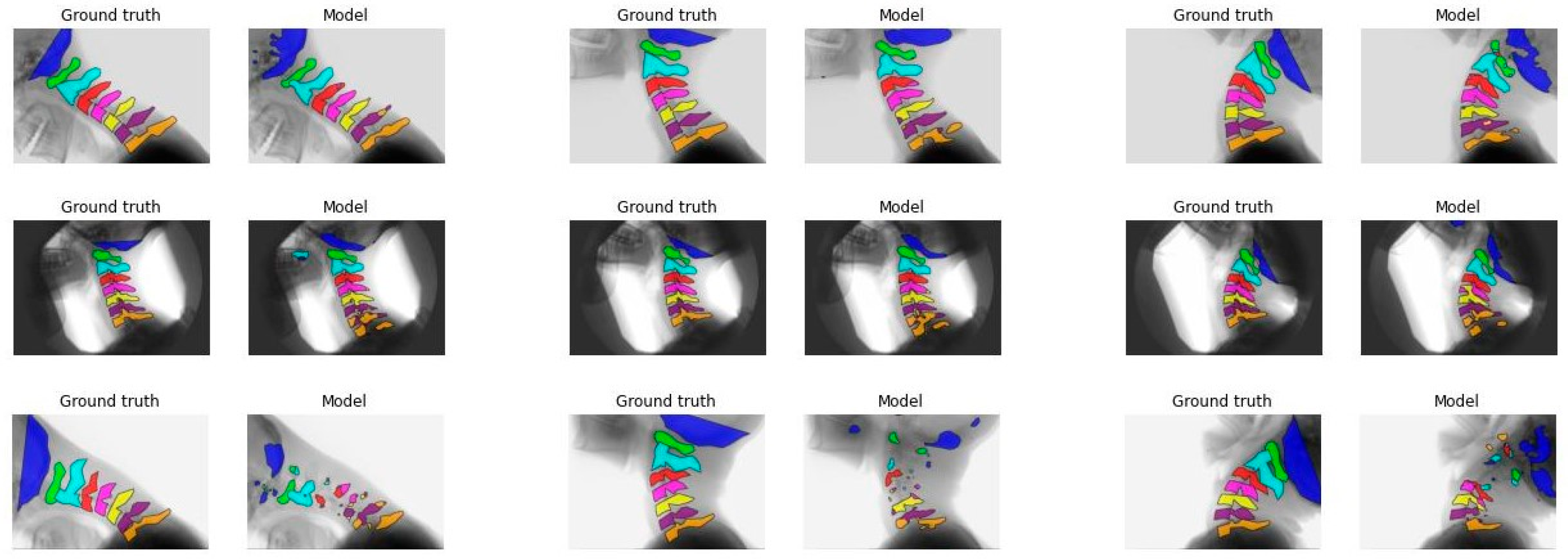
Figure A5.
Comparison between the ground truth and the segmentation made by model D. Each vertebra is indicated with another color. From left to right: first-median-last frame of the recording. From top to bottom, the comparison with the best visual comparison to the worst visual comparison.
Figure A5.
Comparison between the ground truth and the segmentation made by model D. Each vertebra is indicated with another color. From left to right: first-median-last frame of the recording. From top to bottom, the comparison with the best visual comparison to the worst visual comparison.
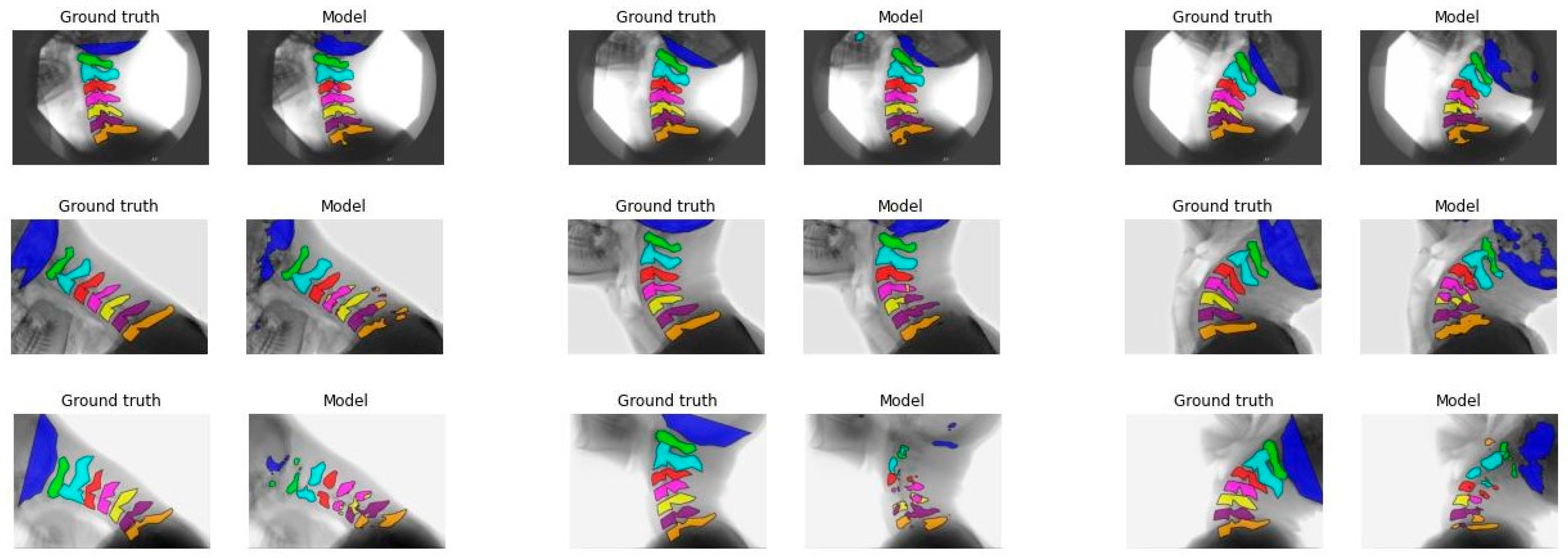
Figure A6.
Mean shape compared to the ground truth of C1-C7. Ground truth is indicated in blue, mean shape is given in red. Overlapping areas appear as purple: (a) Vertebra C1; (b) Vertebra C2; (c) Vertebra C3; (d) Vertebra C4 (e) Vertebra C6; (f) Vertebra C7.
Figure A6.
Mean shape compared to the ground truth of C1-C7. Ground truth is indicated in blue, mean shape is given in red. Overlapping areas appear as purple: (a) Vertebra C1; (b) Vertebra C2; (c) Vertebra C3; (d) Vertebra C4 (e) Vertebra C6; (f) Vertebra C7.
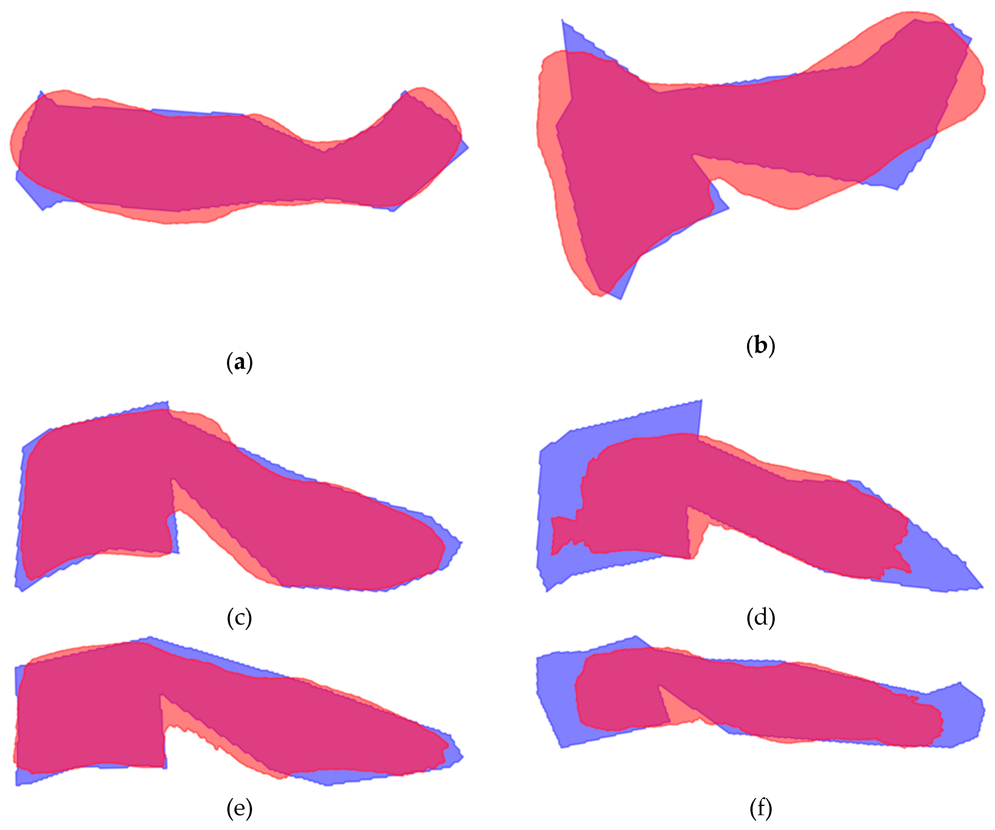
Figure A7.
Mean shape compared to the model segmentation of C1-C7. Model segmentation is indicated in blue, mean shape is given in red. Overlapping areas appear as purple: (a) Vertebra C1; (b) Vertebra C2; (c) Vertebra C3; (d) Vertebra C4 (e) Vertebra C6; (f) Vertebra C7.
Figure A7.
Mean shape compared to the model segmentation of C1-C7. Model segmentation is indicated in blue, mean shape is given in red. Overlapping areas appear as purple: (a) Vertebra C1; (b) Vertebra C2; (c) Vertebra C3; (d) Vertebra C4 (e) Vertebra C6; (f) Vertebra C7.
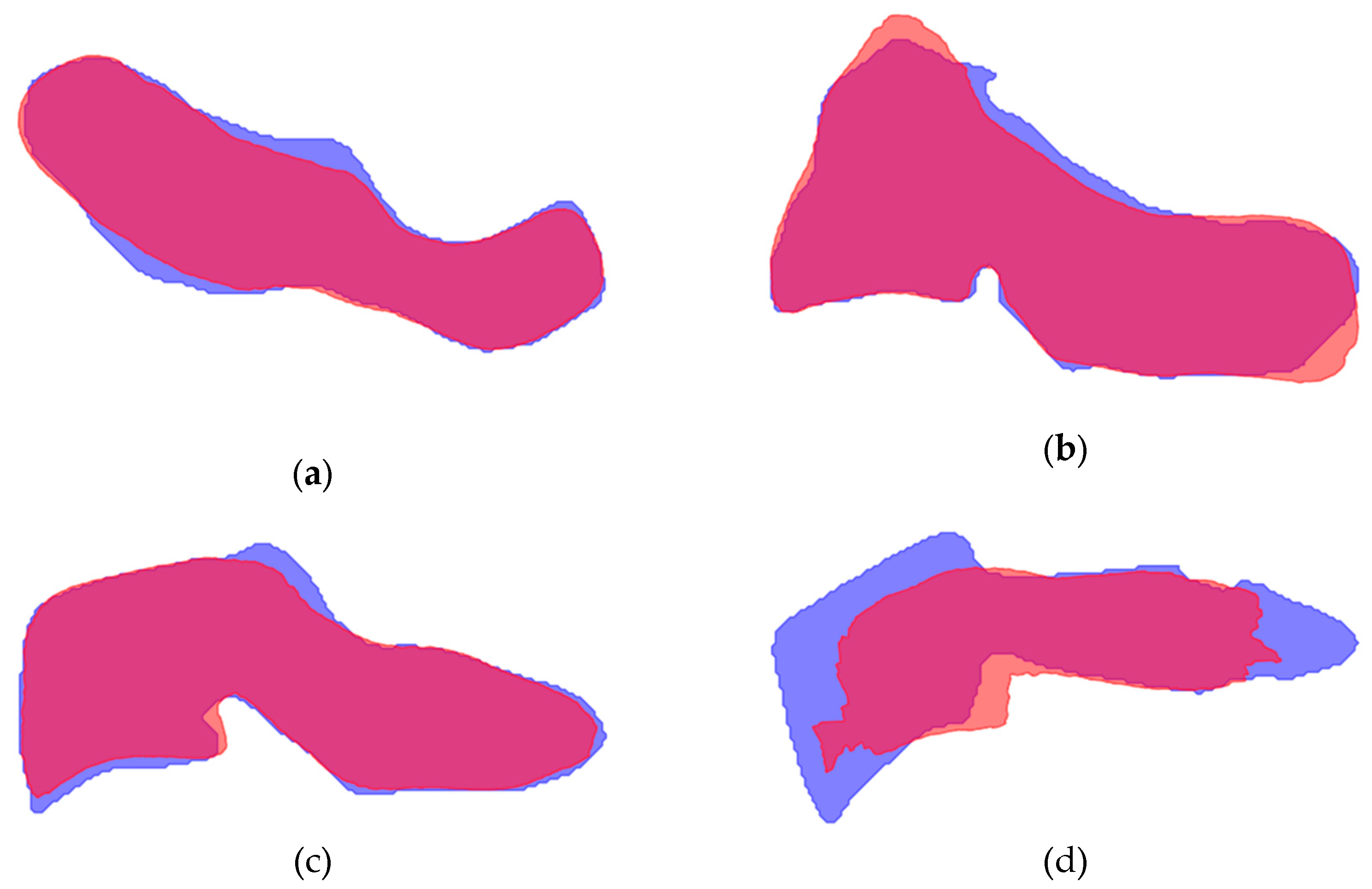
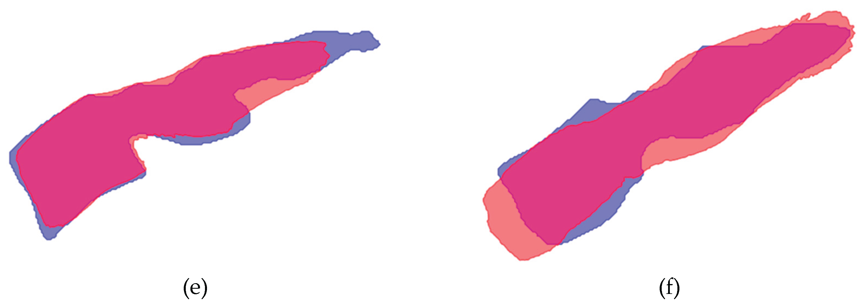
Figure A8.
Median frame of recordings with low performance scores.
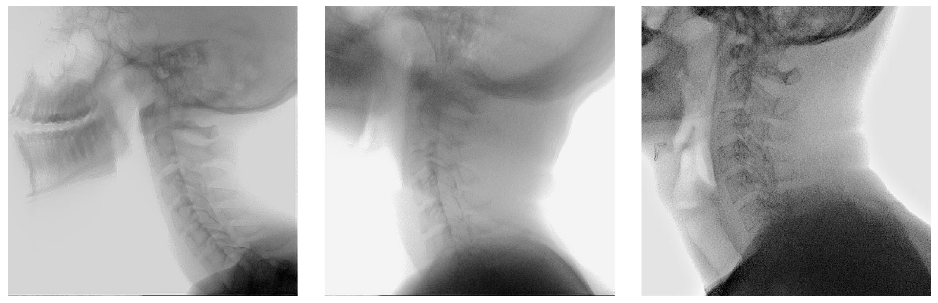
Figure A9.
Median frame of recordings with high performance scores.
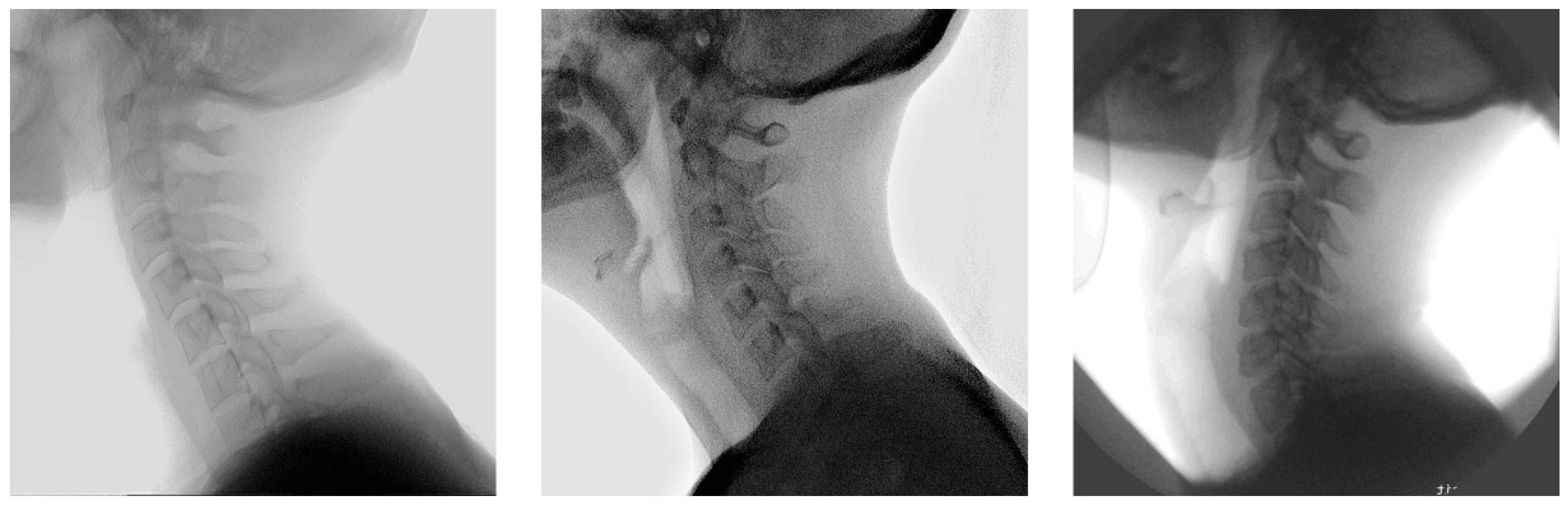
Table A4.
ICC scores for vertebral segments calculated per model using model segmentation.
| Model A | Model B | Model C | Model D | |||||
|---|---|---|---|---|---|---|---|---|
| Segment | ICC [min-max] |
n | ICC [min-max] |
n | ICC [min-max] |
n | ICC [min-max] |
n |
| C1-C2 | 0.143 [0.056-0.218] |
4 | 0.146 [0.081-0.251] |
3 | 0.205 [0.106-0.346] |
3 | 0.082 [0.052-0.112] |
2 |
| C2-C3 | 0.258 [0.139-0.325] |
3 | 0.238 [0.221-0.254] |
2 | 0.178 [0.063-0.344] |
3 | 0.078 [0.022-0.133] |
2 |
| C3-C4 | 0.017 [n/a] |
1 | 0.112 [0.028-0.245] |
3 | 0.018 [0.007-0.063] |
2 | n/a | 0 |
| C4-C5 | n/a | 0 | n/a | 0 | n/a | 0 | 0.1 [0.031-0.069] |
2 |
| C5-C6 | n/a | 0 | 0.003 [n/a] |
1 | n/a | 0 | 0.041 [n/a] |
1 |
| C6-C7 | n/a | 0 | n/a | 0 | n/a | 0 | 0.043 [0.0-0.086] |
2 |
ICC= Intraclass Correlation Coefficient.
References
- Bogduk, N.; Mercer, S. Biomechanics of the cervical spine. I: Normal kinematics. Clin Biomech (Bristol, Avon) 2000, 15, 633–648. [Google Scholar] [CrossRef]
- H., v.M. Motion patterns in the cervical spine; Maastricht University: Maastricht, 1988. [Google Scholar]
- Van Mameren, H.; Drukker, J.; Sanches, H.; Beursgens, J. Cervical spine motion in the sagittal plane (I) range of motion of actually performed movements, an X-ray cinematographic study. Eur J Morphol 1990, 28, 47–68. [Google Scholar]
- Boselie, T.F.M.; van Santbrink, H.; de Bie, R.A.; van Mameren, H. Pilot Study of Sequence of Segmental Contributions in the Lower Cervical Spine During Active Extension and Flexion: Healthy Controls Versus Cervical Degenerative Disc Disease Patients. Spine (Phila Pa 1976) 2017, 42, E642–E647. [Google Scholar] [CrossRef]
- Schuermans, V.N.E.; Breen, A.; Branney, J.; Smeets, A.; van Santbrink, H.; Boselie, T.F.M. Cross-Validation of two independent methods to analyze the sequence of segmental contributions in the cervical spine in extension cineradiographic recordings.
- Boselie, T.F.; van Mameren, H.; de Bie, R.A.; van Santbrink, H. Cervical spine kinematics after anterior cervical discectomy with or without implantation of a mobile cervical disc prosthesis; an RCT. BMC Musculoskelet Disord 2015, 16, 34. [Google Scholar] [CrossRef]
- Schuermans, V.N.E.; Smeets, A.; Curfs, I.; van Santbrink, H.; Boselie, T.F.M. A randomized controlled trial with extended long-term follow-up: Quality of cervical spine motion after anterior cervical discectomy (ACD) or anterior cervical discectomy with arthroplasty (ACDA). Brain Spine 2024, 4, 102726. [Google Scholar] [CrossRef]
- Schuermans, V.N.E.; Smeets, A.; Breen, A.; Branney, J.; Curfs, I.; van Santbrink, H.; Boselie, T.F.M. An observational study of quality of motion in the aging cervical spine: sequence of segmental contributions in dynamic fluoroscopy recordings. BMC Musculoskelet Disord 2024, 25, 330. [Google Scholar] [CrossRef]
- Al Arif, S.; Knapp, K.; Slabaugh, G. Fully automatic cervical vertebrae segmentation framework for X-ray images. Comput Methods Programs Biomed 2018, 157, 95–111. [Google Scholar] [CrossRef]
- Shim, J.H.; Kim, W.S.; Kim, K.G.; Yee, G.T.; Kim, Y.J.; Jeong, T.S. Evaluation of U-Net models in automated cervical spine and cranial bone segmentation using X-ray images for traumatic atlanto-occipital dislocation diagnosis. Sci Rep 2022, 12, 21438. [Google Scholar] [CrossRef]
- Fujita, K.; Matsuo, K.; Koyama, T.; Utagawa, K.; Morishita, S.; Sugiura, Y. Development and testing of a new application for measuring motion at the cervical spine. BMC Med Imaging 2022, 22, 193. [Google Scholar] [CrossRef]
- Avesta, A.; Hossain, S.; Lin, M.; Aboian, M.; Krumholz, H.M.; Aneja, S. Comparing 3D, 2.5D, and 2D Approaches to Brain Image Auto-Segmentation. Bioengineering (Basel) 2023, 10. [Google Scholar] [CrossRef]
- Vu, M.H.; Grimbergen, G.; Nyholm, T.; Lofstedt, T. Evaluation of multislice inputs to convolutional neural networks for medical image segmentation. Med Phys 2020, 47, 6216–6231. [Google Scholar] [CrossRef]
- Branney, J. An Observational study of changes in cervical inter-vertebral motion and the relationship with patient-reported outcomes in patients undergoing spinal manipulative therapy for neck pain; Bournemouth University, 2014. [Google Scholar]
- Branney, J.; Breen, A.C. Does inter-vertebral range of motion increase after spinal manipulation? A prospective cohort study. Chiropr Man Therap 2014, 22, 24. [Google Scholar] [CrossRef]
- Reinartz, R.; Platel, B.; Boselie, T.; van Mameren, H.; van Santbrink, H.; Romeny, B. Cervical vertebrae tracking in video-fluoroscopy using the normalized gradient field. Med Image Comput Comput Assist Interv 2009, 12, 524–531. [Google Scholar] [CrossRef]
- Ronneberger, O.; Fischer, P.; Brox, T. U-Net: Convolutional Networks for Biomedical Image Segmentation. In Proceedings of the Medical Image Computing and Computer-Assisted Intervention – MICCAI 2015, Cham, 2015; pp. 234–241. [Google Scholar]
- Siddique, N.; Paheding, S.; Elkin, C.P.; Devabhaktuni, V. U-Net and Its Variants for Medical Image Segmentation: A Review of Theory and Applications. IEEE Access 2021, 9, 82031–82057. [Google Scholar] [CrossRef]
- Dice, L.R. Measures of the Amount of Ecologic Association Between Species. Ecology 1945, 26, 297–302. [Google Scholar] [CrossRef]
- Zou, K.H.; Warfield, S.K.; Bharatha, A.; Tempany, C.M.; Kaus, M.R.; Haker, S.J.; Wells, W.M., 3rd; Jolesz, F.A.; Kikinis, R. Statistical validation of image segmentation quality based on a spatial overlap index. Acad Radiol 2004, 11, 178–189. [Google Scholar] [CrossRef]
- Kittipongdaja, P.; Siriborvornratanakul, T. Automatic kidney segmentation using 2.5D ResUNet and 2.5D DenseUNet for malignant potential analysis in complex renal cyst based on CT images. EURASIP J Image Video Process 2022, 2022, 5. [Google Scholar] [CrossRef]
- Li, J.; Liao, G.; Sun, W.; Sun, J.; Sheng, T.; Zhu, K.; von Deneen, K.M.; Zhang, Y. A 2.5D semantic segmentation of the pancreas using attention guided dual context embedded U-Net. Neurocomputing 2022, 480, 14–26. [Google Scholar] [CrossRef]
- Gilad, I.; Nissan, M. A study of vertebra and disc geometric relations of the human cervical and lumbar spine. Spine (Phila Pa 1976) 1986, 11, 154–157. [Google Scholar] [CrossRef] [PubMed]
- Choukali, M.A.; Valizadeh, M.; Amirani, M.C.; Mirbolouk, S. A desired histogram estimation accompanied with an exact histogram matching method for image contrast enhancement. Multimedia Tools and Applications 2023, 82, 28345–28365. [Google Scholar] [CrossRef]
- Salvi, M.; Acharya, U.R.; Molinari, F.; Meiburger, K.M. The impact of pre- and post-image processing techniques on deep learning frameworks: A comprehensive review for digital pathology image analysis. Comput Biol Med 2021, 128, 104129. [Google Scholar] [CrossRef] [PubMed]
- Vogt, S.; Scholl, C.; Grover, P.; Marks, J.; Dreischarf, M.; Braumann, U.D.; Strube, P.; Holzl, A.; Bohle, S. Novel AI-Based Algorithm for the Automated Measurement of Cervical Sagittal Balance Parameters. A Validation Study on Pre- and Postoperative Radiographs of 129 Patients. Global Spine J 2024. [Google Scholar] [CrossRef] [PubMed]
Figure 1.
Comparison between the ground truth and the segmentation made by model C. Each vertebra is indicated with another color. From left to right: first-median-last frame of the recording. From top to bottom, the comparison with the best visual comparison to the worst visual comparison.
Figure 1.
Comparison between the ground truth and the segmentation made by model C. Each vertebra is indicated with another color. From left to right: first-median-last frame of the recording. From top to bottom, the comparison with the best visual comparison to the worst visual comparison.
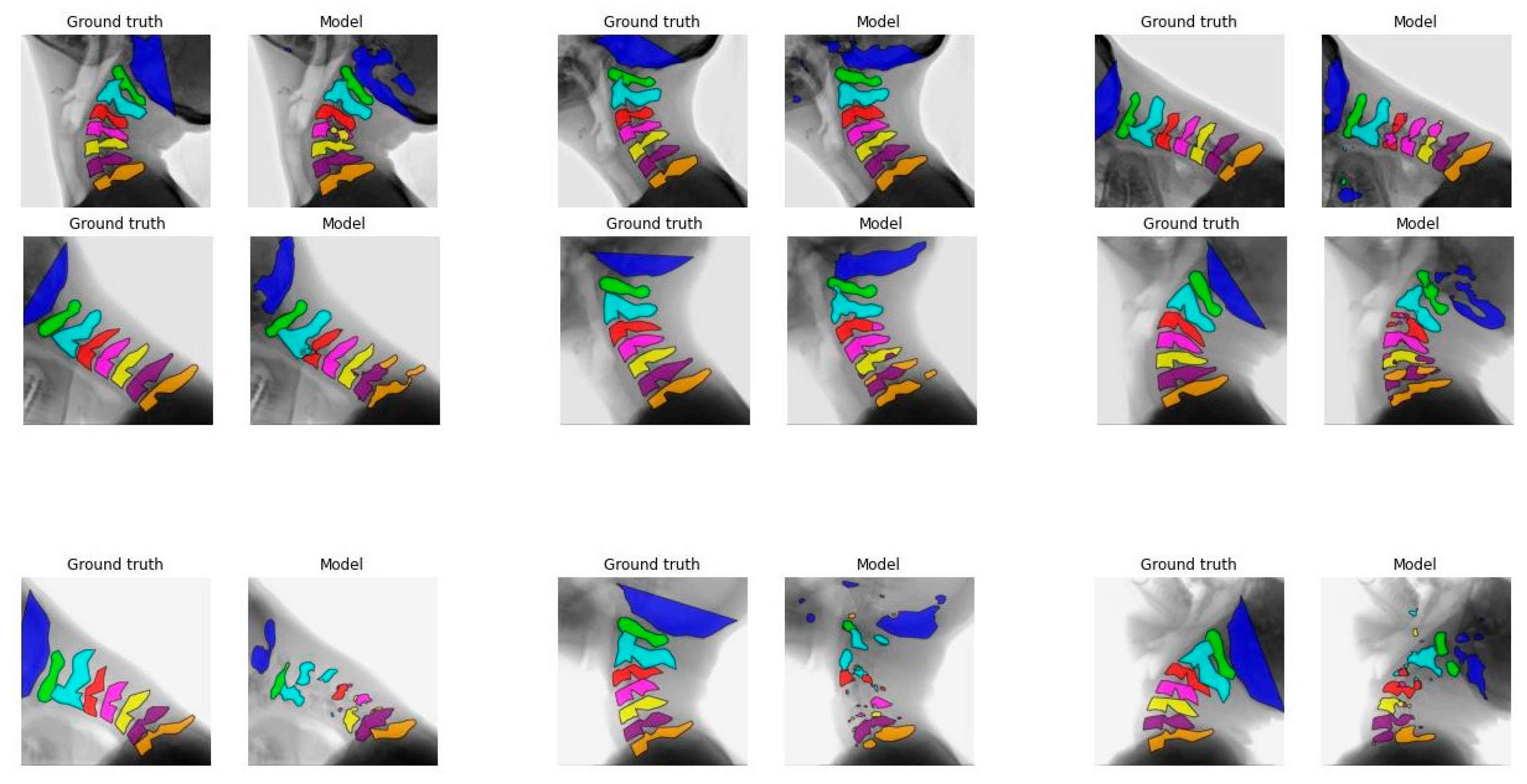
Figure 2.
Visualization of the mean shape of C5. Both a and b are calculated on the median frame. (a) Ground truth is blue, mean shape is red, and overlap is purple; (b) Model segmentation is blue, mean shape is red, and overlap is purple.
Figure 2.
Visualization of the mean shape of C5. Both a and b are calculated on the median frame. (a) Ground truth is blue, mean shape is red, and overlap is purple; (b) Model segmentation is blue, mean shape is red, and overlap is purple.
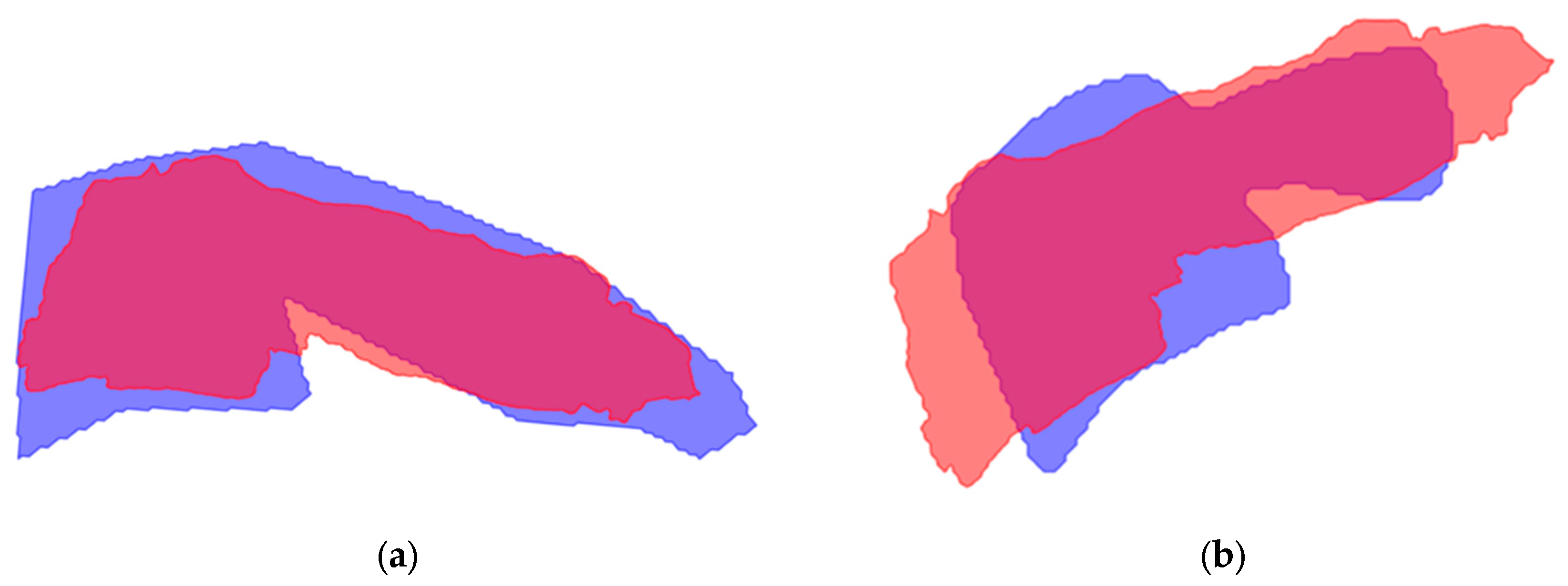
Figure 3.
(a) Visual graph trajectory C1 model A (ICC 0.990); (b) Visual graph trajectory C3 model D (ICC 0.298). Blue line= ground truth, red line= mean shape.
Figure 3.
(a) Visual graph trajectory C1 model A (ICC 0.990); (b) Visual graph trajectory C3 model D (ICC 0.298). Blue line= ground truth, red line= mean shape.
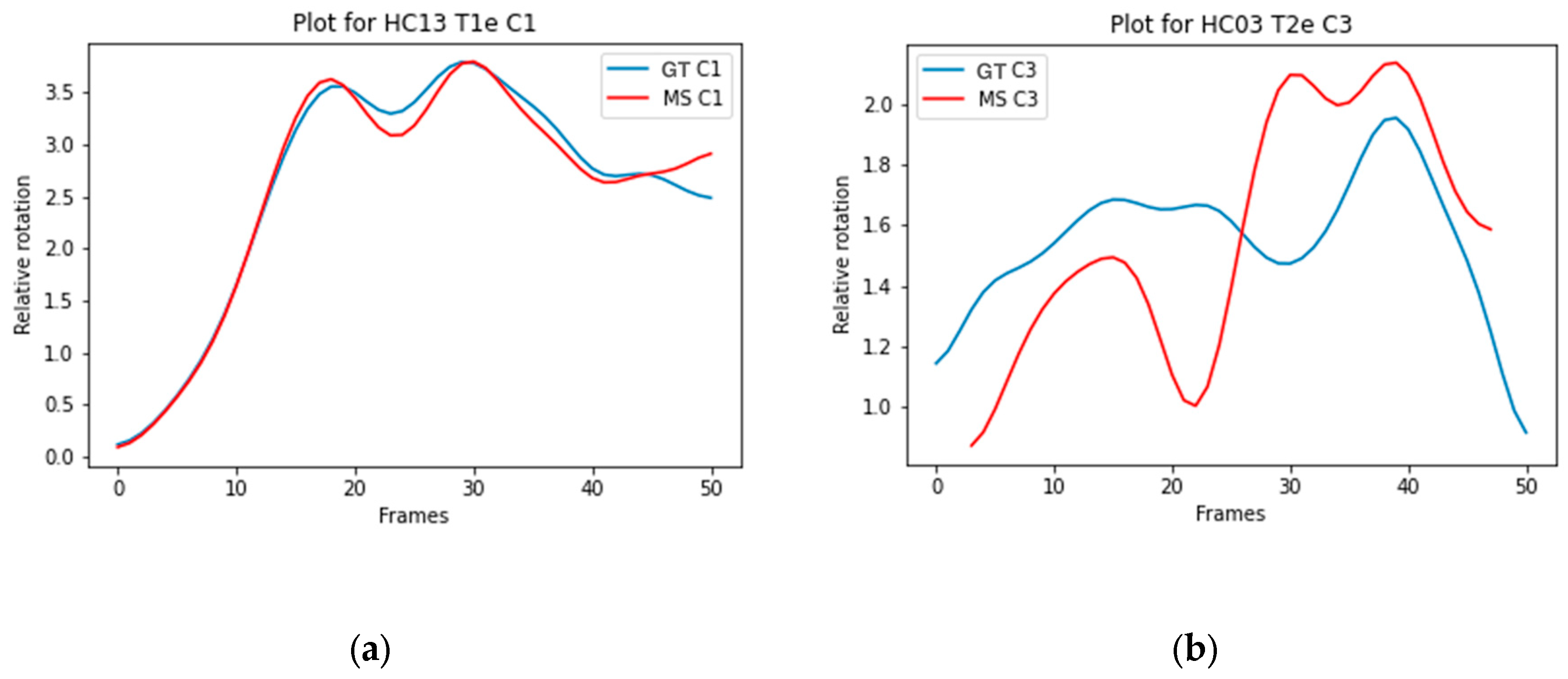
Figure 4.
(a) Visual graph trajectory C1-C2 model D (ICC 0.890); (b) Visual graph trajectory C5-C6 model B (ICC 0.000). Blue line= ground truth, red line= mean shape, yellow line= unfiltered mean shape trajectory.
Figure 4.
(a) Visual graph trajectory C1-C2 model D (ICC 0.890); (b) Visual graph trajectory C5-C6 model B (ICC 0.000). Blue line= ground truth, red line= mean shape, yellow line= unfiltered mean shape trajectory.
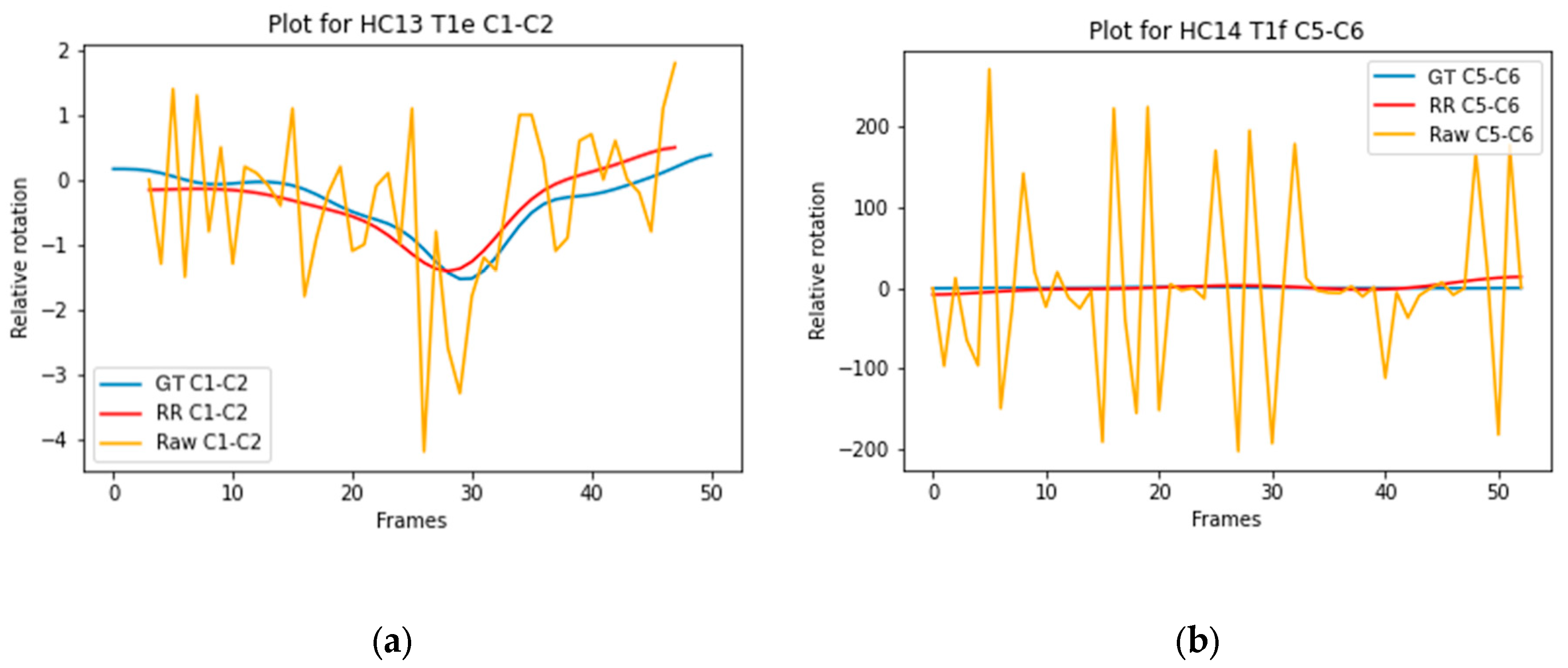
Table 1.
Overview of the tested models A to D.
| Model | Dimension | |
|---|---|---|
| A | 640x640 | 2D |
| B | 832x576 | 2D |
| C | 640x640 | 2D + time |
| D | 832x576 | 2D + time |
Table 2.
Overview of the included data divided into subsets, displayed for number of individuals and number of recordings.
Table 2.
Overview of the included data divided into subsets, displayed for number of individuals and number of recordings.
| Data subset | Individuals (N=) | Recordings (N=) |
|---|---|---|
| Training (55%) | 21 | 52 |
| Validation (20%) | 8 | 18 |
| Testing (25%) | 10 | 19 |
Table 3.
Performance of model options A-D on the test set.
| IoU | DSC | |||||||
|---|---|---|---|---|---|---|---|---|
| Model | A | B | C | D | A | B | C | D |
| C0 | 0.37 | 0.51* | 0.45 | 0.49 | 0.53 | 0.66* | 0.61 | 0.64 |
| C1 | 0.71 | 0.72* | 0.72 | 0.7 | 0.81 | 0.82* | 0.82 | 0.81 |
| C2 | 0.72 | 0.71 | 0.72 | 0.72 | 0.82 | 0.81 | 0.82 | 0.82* |
| C3 | 0.7 | 0.72 | 0.74* | 0.72 | 0.8 | 0.82 | 0.83* | 0.82 |
| C4 | 0.6 | 0.64* | 0.63 | 0.63 | 0.72 | 0.76* | 0.74 | 0.75 |
| C5 | 0.51 | 0.56 | 0.52 | 0.58* | 0.64 | 0.69 | 0.64 | 0.71* |
| C6 | 0.51 | 0.55 | 0.57 | 0.59* | 0.65 | 0.69 | 0.7 | 0.73* |
| C7 | 0.51 | 0.52 | 0.55* | 0.54 | 0.65 | 0.66 | 0.68* | 0.67 |
IoU= Intersection over Union, DSC= Disc Similarity Coefficient. The highest IoU and DSC values for each vertebra are indicated in bold. Significant differences compared to all other options are marked with an asterisk.
Table 4.
The mean IoU score calculated between the ground truth and mean shape of each vertebra, per model A-D.
Table 4.
The mean IoU score calculated between the ground truth and mean shape of each vertebra, per model A-D.
| A | B | C | D | |
|---|---|---|---|---|
| C1 | 0.76 | 0.76 | 0.78 | 0.75 |
| C2 | 0.80 | 0.79 | 0.78 | 0.76 |
| C3 | 0.79 | 0.84 | 0.84 | 0.84 |
| C4 | 0.69 | 0.81 | 0.78 | 0.75 |
| C5 | 0.56 | 0.62 | 0.61 | 0.61 |
| C6 | 0.60 | 0.56 | 0.63 | 0.66 |
| C7 | 0.63 | 0.63 | 0.62 | 0.56 |
IoU= Intersection over Union.
Table 5.
ICC scores individual vertebrae calculated per model using the mean shape.
| Model A | Model B | Model C | Model D | |||||
|---|---|---|---|---|---|---|---|---|
| Vertebra | ICC [min-max] |
n | ICC [min-max] |
n | ICC [min-max] |
n | ICC [min-max] |
n |
| C1 |
0.962 [0.916-0.993] |
7 | 0.948 [0.834-0.996] |
13 | 0.888 [0.471-0.997] |
12 | 0.843 [0.479-0.982] |
12 |
| C2 |
0.904 [0.699-0.996] |
10 | 0.882 [0.449-0.978] |
12 | 0.868 [0.413-0.988] |
12 | 0.796 [0.400-0.985] |
12 |
| C3 | 0.871 [0.422-0.993] |
7 |
0.917 [0.826-0.976] |
9 | 0.741 [0.132-0.979] |
7 | 0.620 [0.298-0.909] |
6 |
| C4 | 0.880 [0.814-0.960] |
3 | 0.812 [0.601-0.927] |
7 |
0.907 [0.899-0.923] |
3 | 0.636 [0.343-0.820] |
3 |
| C5 |
0.904 [n/a] |
1 | 0.798 [0.650-0.945] |
2 | 0.683 [0.658-0.680] |
2 | 0.775 [0.707-0.864] |
3 |
| C6 |
0.982 [n/a] |
1 | 0.830 [0.665-0.995] |
2 | 0.769 [0.471-0.979] |
4 | 0.878 [0.639-0.966] |
8 |
| C7 | 0.819 [0.732-0.905] |
2 | 0.869 [0.650-0.954] |
5 |
0.879 [0.785-0.974] |
5 | 0.863 [0.697-0.942] |
4 |
ICC= Intraclass Correlation Coefficient. Per vertebra the highest mean score is indicated in red bold.
Table 6.
ICC scores for vertebral segments calculated per model using the mean shape.
| Model A | Model B | Model C | Model D | |||||
|---|---|---|---|---|---|---|---|---|
| Segment | ICC [min-max] |
n | ICC [min-max] |
n | ICC [min-max] |
n | ICC [min-max] |
n |
| C1-C2 | 0.685 [0.481-0.988] |
5 | 0.627 [0.136-0.938] |
5 | 0.713 [0.283-0.937] |
7 |
0.724 [0.559-0.890] |
4 |
| C2-C3 | 0.512 [0.181-0.934] |
4 | 0.408 [0.025-0.661] |
4 |
0.500 [0.321-0.615] |
6 | 0.340 [0.006-0.647] |
4 |
| C3-C4 | 0.511 [n/a] |
1 | 0.412 [0.025-0.831] |
5 | 0.382 [0.355-0.409] |
2 |
0.645 [n/a] |
1 |
| C4-C5 | n/a] | 0 | 0.489 [0.464-0.514] |
2 |
0.578 [0.492-0.663] |
2 | 0.281 [n/a] |
1 |
| C5-C6 | n/a | 0 | 0.605 [0.505-0.705] |
2 | 0.535 [n/a] |
1 |
0.542 [0.314-0.772] |
3 |
| C6-C7 | 0.674 [n/a] |
1 | n/a | 0 |
0.770 [n/a] |
1 | 0.685 [n/a] |
1 |
ICC= Intraclass Correlation Coefficient. Per vertebra the highest mean score is indicated in red bold.
Disclaimer/Publisher’s Note: The statements, opinions and data contained in all publications are solely those of the individual author(s) and contributor(s) and not of MDPI and/or the editor(s). MDPI and/or the editor(s) disclaim responsibility for any injury to people or property resulting from any ideas, methods, instructions or products referred to in the content. |
© 2025 by the authors. Licensee MDPI, Basel, Switzerland. This article is an open access article distributed under the terms and conditions of the Creative Commons Attribution (CC BY) license (http://creativecommons.org/licenses/by/4.0/).
Copyright: This open access article is published under a Creative Commons CC BY 4.0 license, which permit the free download, distribution, and reuse, provided that the author and preprint are cited in any reuse.


