Submitted:
12 May 2025
Posted:
12 May 2025
You are already at the latest version
Abstract
We investigate the partial differential equation system which describes the double-diffusion convection phenomena with the reduction formalism.
Double-diffusion means when two scalar quantities with different diffusivities, such as heat and solute concentration, contribute
to density gradients within a fluid under the influence of gravity.
The time-dependent self-similar trial function is applied and analytic results are presented and analyzed in details.
Keywords:
diffusion
; double-diffusion
; self-similar solution
1. Introduction
There is no question that transport processes have extreme importance both for scientific and engineering applications. The simplest ones are heat conduction in solids and the regular diffusion of particles. The existing literature of diffusion (or of heat conduction) is immense; therefore, we mention some recent monographs [1,2,3,4,5,6], only. The development in numerical analysis of diffusion equations made remarkable steps in the last years as well [7]. On the other side the mathematical generalization of the diffusion equation including the p-Laplacean was investigated also [8,9].
Coupling additional transport mechanisms (like fluid flow) to regular diffusion or heat conduction drastically opens the horizon of interesting phenomena and non-linear effects. Nice examples are simplified heated flow systems like heated boundary layers [10] or the Rayleigh-Bènard convection [11]. These are diffusive convection systems where heat is transported together with particle flow which is convection instead of conduction. Such processes are extremely important in the science of meteorology [12] oceanography [13] or in climate change studies [14].
More than half a century ago E.N. Lorenz’s investigated the Rayleigh-Bènard convection [15] and with a truncated Fourier series as a trial function he pioneered the way to a new discipline called chaos theory. On the other way, if we investigate such diffusive convection systems with the self-similar Ansatz we can relatively easily derive analytic solutions which can predict the asymptotic temporal or spatial behavior of such physical phenomena. The self-similar Ansatz is the natural trial function of the regular diffusion equation [16] because the fundamental or Gaussian solution can be derived in a few lines and astonishingly new kind of solutions can be easily obtained as well. This strong performance of this function gives us a strong hint that additional disperse dynamical systems can be successfully analyzed giving insight into the global properties of their solutions. In the last years we successfully investigated such systems like the Rayleigh-Bènard convection [17] or heated boundary layers [18] presenting physically relevant analytic solutions in connection to different special functions like the Kummer’s M and Kummer’s U functions.
We can continue on this path defining more complex (or rather more compound) systems and investigate how they behave. First we analyzed systems where some diffusion equations were coupled in various ways [19].
In the next study we consider the double-diffusive convection which is a fundamental fluid dynamics phenomenon that arises when two scalar quantities with different diffusivities, such as heat and solute concentration, contribute to density gradients within a fluid under the influence of gravity. The interplay between thermal and compositional buoyancy forces gives rise to a rich variety of flow patterns and instabilities, which are often more complex than those observed in single-component convection. Understanding the mathematical structure and behavior of the double-diffusive convection equation system is therefore essential for both theoretical and applied sciences. Therefore a detailed linear stability analysis of double-diffusive convection was performed, laying the groundwork for understanding the onset of instabilities [20]. The low Prandtl number flow behavior which is relevant to astrophysical and geophysical applications was exhaustively studied as well [21]. The sub-microscale dynamics of double-diffusive convection was investigated recently by Radko [22]. Additional effects in homogeneous and heterogeneous porous media are also the subject of current investigations [23].
The literature of this field is remarkable extensive, without completeness we just mention some relevant studies and monographs [24,25,26,27]. Double-diffusion process is an important process in oceanography in general [28], in geophysics understanding the phenomena in magma chambers [29], in astrophysics [30,31,32], or double-diffusive magnetic layering [33]. In hydrology it is meant to describe sediment laden rivers in lakes and the ocean [34,35] in metallurgy [36] or finally even in various engineering applications [37,38]. The formation of salt deposits, under salt density gradient and the presence of solar radiation, have been studied in [39]. The salinity gradient also implies typically a manifestation of bacterial diversity in lakes. Different bacteria may be present in lakes, depending on depth and salinity concentration [40]. Combined effects of salt diffusion, in food industry, have been also studied [41].
After the very first analysis of "an oceanographic curiosity: the perpetual salt fountain" by Henry Stommel and co-workers in 1956 [42], Stern in 1960 firstly described the double-diffusive convection and introduced the concept of salt fingers and their role in oceanographic processes [43].
It is clear that the most studied double-diffusion system is salty fingers. The question of the limits on growing finite–length salt fingers was analyzed and a Richardson number constraint was found by [44]. Planform selection in salt fingers was also studied [45].
Additionally - again without completeness - we mention some references for the interested reader [46,47,48].
This publication aims to contribute to the ongoing exploration of the mathematics of double-diffusive convection by presenting new analytical results that shed light on the system’s behavior across different parameter regimes. By elucidating the underlying mechanisms and mathematical structure of this complex phenomenon, we hope to advance both the theoretical understanding and practical control of double-diffusive systems in nature and industry.
2. Theory and Results
2.1. Double-Diffusion System with No Extra Source Terms
The conservation equations for mass, vertical momentum, heat and salinity equations (under Boussinesq’s approximation) which describes double diffusive salt finger can be formulated in general vector form [46]. We want to perform direct calculations, correspondingly we start with following system of differential equations:
applying the standard notation therefore and S denote the dynamical variables of the horizontal and vertical speed components, the temperature and the salinity. The physical parameters and are the kinematic viscosity, the gravitational acceleration, the coefficient of thermal expansion, the haline concentration coefficient at constant pressure and temperature, the molecular diffusivity of heat and the molecular diffusivity of salt [49]. We suppose that all the above mention coefficients are constant for the system studied. There are also cases where the diffusion or heat diffusion coefficient may depend on the parameters of the problem [50,51]. (The complete analysis or the realistic equation-of-state for sea water is a very complicated problem having a large literature. Fortunately these aspects are irrelevant for our forthcoming analysis.) Consider Figure (Figure 1) to fix our system’s geometrical relations.
All five physical parameters should have positive real values. For the better transparency we use the subscripts for the corresponding partial derivatives. The horizontal and the vertical space variables are denoted with x and z, respectively.
In the next we apply the generalization of the self-similar Ansatz [52] for two Cartesian space dimensional dependent dynamical variables in the form of:
where is the reduced variable. In the next we demand the existence of the corresponding first and second derivatives of the shape functions with adequate smoothness. (We usually use the first two Greek letters and for the self-similar exponents as well but now these are fixed to physical parameters.) The exponent is responsible for the spreading of the dynamical variable in time, and all the other four exponents describe the decay or increment of the variable in time. In most of the cases positive exponents mean spreading and decaying solutions in time, which meets our physical intuitions. Existing self-similar symmetry also means that the investigated system has no additional characteristic relaxation time or characteristic length. It is also true that self-similar solutions are defined on infinite horizon and there is no need to introduce dimensionless variable like in the work of [46]. For infinite horizon it is not possible to define reasonable Reynolds or Rayleigh numbers.
After the usual steps of algebraic manipulations we arrive to the ordinary differential equation (ODE) system of
where prime means derivation with respect to . Additionally we get some constraints among the self-similar exponents:
Note, that now all exponents got the same fixed numerical value, which means that the mathematics of the solution is quite restricted. If some exponents remain free then the ODE system and the final solutions contain them as free parameters, too. For the regular diffusion equation if both exponents are fixed to one half we automatically get fundamental Gaussian and error function solutions. It is worth to mention here, that the Rayleigh-Bènard convection model [17] (which in a sense is a far analog) of this systems has slightly different self-similar exponents resulting much richer mathematical structure. Now only, the original physical parameters of the starting dynamical system remain free. As usual the ordinary differential equation of the shape function of the continuity equation Equation (7) can be integrated giving us: where c is our first free real integral constant which is proportional to the velocity of the flow. These conditions help us to decouple the heat and the salinity equations from the momentum and the continuity equation. We get even more, the heat conduction and the salinity equations become linear not depending on the products of dynamical variables. Both become independent in the form of
The solutions can be easily obtained by integrating the ODEs giving:
where erf means the Gaussian error function now with imaginary argument, the real integration constants are notated with . For more information about the properties of the error function consult the handbook of [53]. Figure 2a) presents the shape functions of Equation (15) for some parameter sets. The numerical value of c which is basically the velocity, enhances the maximum of the peak and makes a shift to the right of the peak. The molecular diffusivity of salt is responsible for the half-width at half maximum (FWHM) of the peak. Figure 2b) shows the projection of the salinity distribution . This is very similar to the usual Gaussian solution of diffusion.
Now, if the second derivatives of Equations (14) and (15) are derived and replaced into Equation (16) then the momentum equation of the double diffusive convection problem can be solved. Note that the possible integration of the continuity equation may lead to a linear momentum equation; which will also mean in the next that the linear combination of solutions (superposition) will also give us further solutions. Our experience shows, that fully analytic solutions can be evaluated only for in the reverse condition the solution contains an additional integration which should be evaluated numerically when all parameters have a given numerical value. No fully analytic solutions exist for the most general case where all integral constants are not zero. We analyze the real solutions only. Therefore the ODE for the velocity shape function contains just the second derivatives of the exponential function and reads as follows:
The solution can be derived with quadrature and has the form of:
We analyze the real solutions only, therefore we set . It is easy to see, that for , and the two exponential functions cancel each other, because of the two opposing competing diffusion effects. The and are still responsible for the FWHM of the peaks. It is also clear from the formula that for the velocity function becomes infinite. Large viscosity causes small velocity because it stands in the denominator. Figure 3a) shows us two different shape functions with different parameter sets. We can see different kind of linear combinations of exponential-type of functions (note that there is the product of a Gaussian and an exponential function in the formula) the results are now so exciting. Either we have a peak with a global maximum or minimum or two peaks with a minimum in between.
Figure 3b) presents the velocity distribution for the parameters of the black curve. Note, that the exponent is responsible for the quick temporal decay.
To emphasize the linearity of the velocity distribution Equation (16) Figure 4 presents a linear combination of three real solutions of Equation (17) for different integration constants and when the spatial coordinates are shifted. In principle arbitrary large number of solutions could be summed up resulting very complex velocity distributions in double-diffusive convection systems.
2.2. The Role of Possible Source Terms
We can see, that our obtained self-similar solutions are far from being complicated and have no extra peculiarity. This is due to the fixed numerical values of all self-similar exponents. The Rayleigh- Bénard convection which is also a fluid dynamical system with coupled heat conduction has a much broader self-similar symmetry because one of the self-similar exponents remain free. Groping in this direction to generalize the double-diffusive convection system we may consider addition terms like a source in the temperature convection equation.
A straight forward way is taking a source term which is an arbitrary function of the temperature , in this sense Equation (3) is changed to:
Keeping all exponents fixed to it can be easily shown that the linear source terms should have the form of . Here d is the strength of the source (if positive) or sink (when negative) and it fixes the proper physical dimension. The time-dependent factor is needed to have the proper temporal asymptotic. We tried additional power-law dependent source terms as well, only the square root has trivial analytic solution of (We can easily imagine a periodic driving term as well, but that should assume a traveling wave analysis which could the topic of a possible forthcoming analysis. Such systems usually have Mathieu functions in their solutions.) Interesting reconstructions of initial conditions with possible source in diffusion problems one may find in Ref. [54].
Considering the transformation the singularity can be shifted having smooth functions. The corresponding ODE for the temperature shape function is now slightly changed to:
positive d values mean source The solutions read as:
where and are the Kummer’s M and Kummer’s U functions with the usual integral constants of and . For more information about Kummer’s functions see [53].
As definition consider the series expansion of
with the which is the so-called rising factorial or Pochhammer’s Symbol [53]. In our present case b has a fix non-negative integer value, so none of the solutions have poles at . For the Kummer’s function M when the parameter a has negative integer numerical values () the solution is reduced to a polynomial of degree m for the variable z. In other cases we get a convergent infinite series for all values of and z. There is a connecting formula between the two Kummer’s functions, U is defined from M via
where is the Gamma function [53]. It is clear that the structure of the irregular Kummer’s U function is much more complicated.
These very nice mathematical formulas do not help us much to visualize and to imagine how these functions look like for different parameters especially for quadratic arguments. Therefore we present them for some parameter values. Figure 5a) presents the regular Kummer’s M function parts of the solution Equation (20) for different d source values. The c former integral constants means just a shift parallel to the x axis, parameter defines the widths of the solutions. All these functions are real and regular in the origin.
It is important to emphasize that there are four parameter ranges exist where the derived solutions behave qualitatively different:
-
where the derived solutions are divergent for large s, these are the cyan and the gray lines on Fig 3a). If the first parameter of the Kummer’s M function is a negative integer then the function is a finite order polynomial in . A nice example is whereNote, that the first term on the right hand side is a constant, (Formally Kummer’s function of the first kind is equivalent to the generalized confluent hypergeometric series with the notation of 1.)The smaller the first negative parameter of the Kummer’s function the larger the power of the polynomial. Thank to the exponent the final temperature distribution will be decaying, but we will see that not this parameter regime will attract the largest interest among the solutions.
- the solution is constant on the whole axis, this is presented by the brown line.
- the solution is positive on the whole axis, and has a decay to zero at large s such solutions are plotted with pink and green lines. These are well-behaving solutions with a global maxima in the origin, and in this sense similar to Gaussian solutions.
-
the solutions has a maxima in the origin following quick oscillatory decay to zero with growing number of zero transitions as d growing. Black, blue and read curves present such solutions. Unfortunately, the defining series of the Kummer’s M function Equation (21) converges very slowly for highly oscillatory functions.In some sense these are the most interesting solutions.
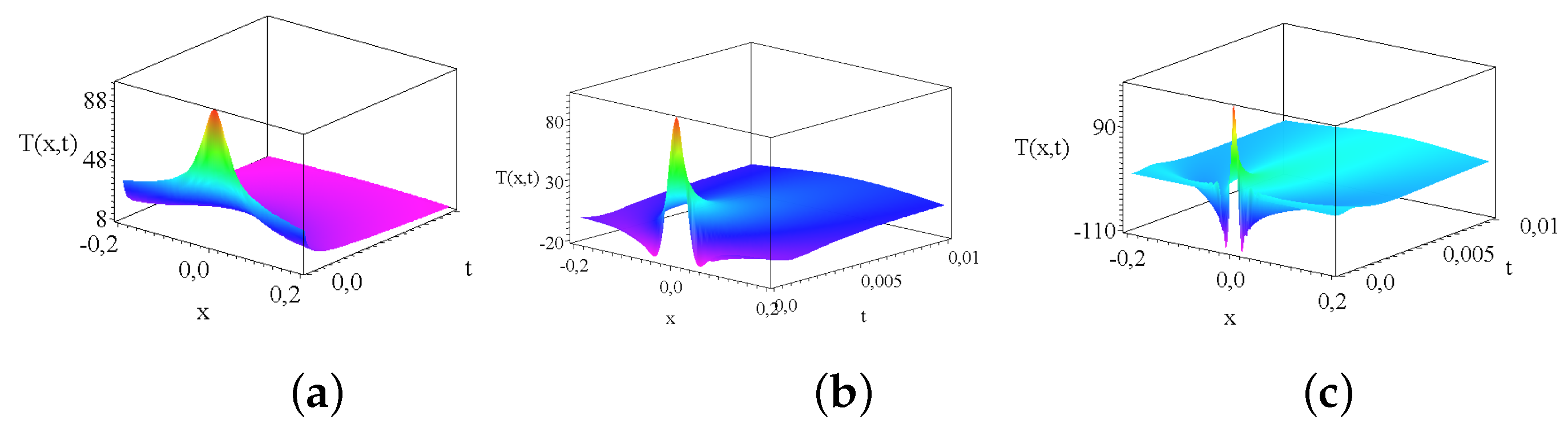
For completeness we show on Figure 5b) how the irregular Kummer’s U solutions behave. It can be shown that the Kummer’s U functions with quadratic argument are finite polynomials is the first arguments are negative integer or half integer values. We present only the real part of the solutions. Note, that the general properties are very similar. There are oscillatory and decaying solutions. There are divergent solutions and there is a finite constant and a constantly zero solution as well. To have a complete overview, Figure 6 shows three temperature distributions given with the Kummer’s M functions. We considered, physically relevant decaying solutions in three different parameter regimes.
We gained plenty of experience with the Kummer’s function [16,17,18,19] in the last years. Usually, an additional Gaussian weight functions was involved in the solutions, but the general properties were very similar. The main difference to our former solution is that, in that now a physical parameter (strength of the heat source) works as an index of the solution and additionally we always have a prefactor in the final dynamical variable which automatically gives us a temporal decay at infinite times.
To complete our investigations we have to analyze the behavior of the velocity field. Considering only real solutions we take the Gaussian solution for the salinity and the Kummer’s M functions for the heat distribution, we can formulate the final ODE:
For a better transparency we just marked and not completed the second derivatives in the equation. Unfortunately, we could not find closed form for the solutions for general Kummer’s functions. However, if the power of the series of Kummer’s function is not larger than four then the ODE has an exact solution.
where the coefficients depend on the parameters of in a complicated way. The solution is exhaustive long and contains numerous Gaussian and error function terms. The direct form is given in the Appendix at the end of the study.
3. Summary and Outlook
We investigated the double diffusion convection flow system, which means that two competing diffusion processes are coupled to the momentum equation. Such real processes are heat and salt convection in water. Our self-similar Ansatz easily gave the Gaussian and error functions for the salinity, temperature and flow velocity distributions, which are less than our former expectations. The reason is that all self-similar exponents had a given value. To deepen our analysis we considered an additional cooler or heater source term in the temperature convection equation which drastically opened the horizon of the possible solutions. The heat distribution function becomes the Kummer’s M or Kummer’s U function. The strength of the heat source becomes the first parameter of the temperature distribution which is a well-understood mathematical feature. Unfortunately, the final velocity distribution cannot be evaluated analytically for all temperature distribution parameters, however it was possible up to a considerable order of expansion of the function of the temperature.
4. Appendix
As a direct example consider
after performing the double differentiation we get:
We name the first constant term of the right hand side with ’A’ after substituting this formula to Equation (24) the solution can be derived with quadrature thanks to Maple 12. Additional exhausting simplification by hand gives us:
Note, that the solution contains Gaussian, exponential, and type dependencies only. The complication comes from the large number of parameters.
Author Contributions
Both authors contributed equally to every part of the study. The first author (Imre Ferenc Barna) had the original idea of the study, performed all the calculations, created the figures and wrote large part of the manuscript. László Mátyás checked the calculations, the collected some part of the cited literature, corrected the manuscript, gave general remarks, evaluated the long time behavior of the solutions and had an everyday contact with the corresponding author.
Funding
This research received no extra founding.
Data Availability Statement
All used data are given in the manuscript.
Conflicts of Interest
The authors declare no conflicts of interest.
References
- Ghez, R. Diffusion Phenomena; Dover Publication Inc: New York, 2001. [Google Scholar]
- Vogel, G. Adventure Diffusion; Springer: New York, 2019. [Google Scholar] [CrossRef]
- Bunde, A.; Caro, J.; Kärger, J.; Vogl, G. Diffusive Spreading in Nature, Technology and Society; Springer Cham: Berlin, 2018. [Google Scholar] [CrossRef]
- Thambynayagam, R. The Diffusion Handbook: Applied Solutions for Engineers; McGraw-Hill: New York, 2011. [Google Scholar]
- Latif, M. Heat Convection; Springer: Berlin, 2009. [Google Scholar] [CrossRef]
- Ashan, A. Convection and Conduction Heat Transfer; Intec: London, 2011. [Google Scholar] [CrossRef]
- Kovács, E. A class of new stable, explicit methods to solve the non-stationary heat equation. Numerical Methods for Partial Differential Equations 2021, 37, 2469–2489. [Google Scholar] [CrossRef]
- Bognár, G.; Rozgonyi, E. The local analytic solution to some nonlinear diffusion-reaction problems. WSEAS Trans. Math. 2008, 7, 382–395. [Google Scholar]
- Guedda, M.; Véron, L. Bifurcation phenomena associated to the p-Laplace operator. Trans. Amer. Math. Soc. 1988, 310, 419–431. [Google Scholar] [CrossRef]
- Schlichting, H.; Gersten, K. Boundary-layer theory; Springer-Verlag: Berlin Heidelberg New York, 2016. [Google Scholar] [CrossRef]
- Goluskin, D. Internally Heated Convection and Rayleigh-Bénard Convection; Springer: New York, 2015. [Google Scholar] [CrossRef]
- Wilford Zdunkowski, A.B. Dynamics of the Atmosphere: A Course in Theoretical Meteorology; Cambridge University Press: Cambridge, 2016. [Google Scholar] [CrossRef]
- Tartar, L. An Introduction to Navier Stokes Equation and Oceanography; Springer: New york, 2006. [Google Scholar] [CrossRef]
- John, H. Seinfeld, S.N.P. Atmospheric Chemistry and Physics, From Air Polution to Climate Change; Wiley-Interscience: New York, 1997. [Google Scholar]
- Lorenz, E.N. Deterministic Nonperiodic Flow. Journal of Atmospheric Sciences 1963, 20, 130–141. [Google Scholar] [CrossRef]
- Mátyás, L.; Barna, I.F. General Self-Similar Solutions of Diffusion Equation and Related Constructions. Romanian Journal of Physics 2022, 67, 101–117. [Google Scholar]
- Barna, I.F.; Mátyás, L. Analytic self-similar solutions of the Oberbeck–Boussinesq equations. Chaos, Solitons & Fractals 2015, 78, 249–255. [Google Scholar] [CrossRef]
- Barna, I.F.; Bognár, G.; Mátyás, L.; Hriczó, K. Self-similar analysis of the time-dependent compressible and incompressible boundary layers including heat conduction. Journal of Thermal Analysis and Calorimetry 2022, 147, 13625–13632. [Google Scholar] [CrossRef]
- Barna, I.F.; Mátyás, L. Diffusion Cascades and Mutually Coupled Diffusion Processes. Mathematics 2024, 12, 3298. [Google Scholar] [CrossRef]
- Baines, P.G.; Gill, A. On thermohaline convection with linear gradients. J. Fluid Mech 1969, 37, 289–306. [Google Scholar] [CrossRef]
- Garaud, P. Double-Diffusive Convection at Low Prandtl Number. Annual Review of Fluid Mechanics 2018, 50, 275–298. [Google Scholar] [CrossRef]
- Radko, T. The sub-microscale dynamics of double-diffusive convection. Journal of Fluid Mechanics 2024, 982. [Google Scholar] [CrossRef]
- Hu, C.; Yang, Y. Double-diffusive convection with gravitationally unstable temperature and concentration gradients in homogeneous and heterogeneous porous media. Journal of Fluid Mechanics 2024, 999, A62. [Google Scholar] [CrossRef]
- Siegmann, W.L.; Rubenfeld, L.A. A Nonlinear Model for Double-Diffusive Convection. SIAM Journal on Applied Mathematics 1975, 29, 540–557. [Google Scholar] [CrossRef]
- Vafai, K. Handbook of porous media; CRC Press: Boca Raton, 2000; chapter Mojtabi, A.; Charrier-Mojtabi, M.-C., Double-Diffusive Convection in Porous Media. [Google Scholar] [CrossRef]
- Radko, T. Double-Diffusive Convection; Cambridge University Press: Cambridge, 2013. [Google Scholar] [CrossRef]
- Alan Brandt, H.F. Double-Diffusive Convection; American Geophysical Union: New York, 1995. [Google Scholar] [CrossRef]
- Schmitt, R.W. Double Diffusion in Oceanography. Annual Review of Fluid Mechanics 2003, 26, 255–285. [Google Scholar] [CrossRef]
- Huppert, H.E.; Sparks, R.J. Double-Diffusive Convection Due to Crystallization in Magmas. Annual Review of Earth and Planetary Sciences 1984, 12, 11–37. [Google Scholar] [CrossRef]
- Leconte, J. .; Chabrier, G.. A new vision of giant planet interiors: Impact of double diffusive convection. A&A 2012, 540, A20. [Google Scholar] [CrossRef]
- Garaud, P. Double-Diffusive Convection at Low Prandtl Number. Annual Review of Fluid Mechanics 2018, 50, 275–298. [Google Scholar] [CrossRef]
- Mirouh, G.M.; Garaud, P.; Stellmach, S.; Traxler, A.L.; Wood, T.S. A NEW MODEL FOR MIXING BY DOUBLE-DIFFUSIVE CONVECTION (SEMI-CONVECTION). I. THE CONDITIONS FOR LAYER FORMATION. The Astrophysical Journal 2012, 750, 61. [Google Scholar] [CrossRef]
- Hughes, D.W.; Brummell, N.H. Double-diffusive Magnetic Layering. The Astrophysical Journal 2021, 922, 195. [Google Scholar] [CrossRef]
- Parsons, J.D.; Bush, J.W.M.; Syvitski, J.P.M. Hyperpycnal plume formation from riverine outflows with small sediment concentrations. Sedimentology 2001, 48, 465–478. [Google Scholar] [CrossRef]
- Davarpanah Jazi, S.; Wells, M.G. Enhanced sedimentation beneath particle-laden flows in lakes and the ocean due to double-diffusive convection. Geophysical Research Letters 2016, 43, 10,883–10,890. [Google Scholar] [CrossRef]
- Schmitt, R.W. The characteristics of salt fingers in a variety of fluid systems, including stellar interiors, liquid metals, oceans, and magmas. The Physics of Fluids 1983, 26, 2373–2377. [Google Scholar] [CrossRef]
- Turner, J.S. Double-Diffusive Phenomena. Annual Review of Fluid Mechanics 1974, 6, 37–54. [Google Scholar] [CrossRef]
- Turner, J.S. Multicomponent Convection. Annual Review of Fluid Mechanics 1985, 17, 11–44. [Google Scholar] [CrossRef]
- Debure, M.; Lassin, A.; Marty, N.; Claret, F.; Virgone, A.; Calassou, S.; Gaucher, E. Thermodynamic evidence of giant salt deposit formation by serpentinization: an alternative mechanism to solar evaporation. Scientific Reports 2019, 9, 11720. [Google Scholar] [CrossRef] [PubMed]
- Máthé, I.; Borsodi, A.K.; Tóth, E.M.; Felföldi, T.; Jurecska, L.; Krett, G.; Kelemen, Z.; Elekes, E.; Barkács, K.; Márialigeti, K. Vertical physico-chemical gradients with distinct microbial communities in the hypersaline and heliothermal Lake Ursu (Sovata, Romania). Extremophiles 2014, 18, 501–514. [Google Scholar] [CrossRef]
- Gyenge, L.; Erdo, K.; Albert, C.; Éva, L.; Salamon, R.V. The effects of soaking in salted blackurrant wine on the properties of cheese. Heliyon 2024, 10, e34060. [Google Scholar] [CrossRef]
- Stommel, H.; Arons, A.B.; Blanchard, D. An oceanographical curiosity: the perpetual salt fountain. Deep Sea Research 1956, 3, 152–153. [Google Scholar] [CrossRef]
- Stern, M.E. The “Salt-Fountain” and Thermohaline Convection. Tellus 1960, 12, 172–175. [Google Scholar] [CrossRef]
- Kunze, E. Limits on growing, finite-length salt fingers: A Richardson number constraint. Journal of Marine Research 1987, 45, 533–556. [Google Scholar] [CrossRef]
- Proctor, M.R.E.; Holyer, J.Y. Planform selection in salt fingers. Journal of Fluid Mechanics 1986, 168, 241–253. [Google Scholar] [CrossRef]
- Schmitt, R.W. The growth rate of super-critical salt fingers. Deep Sea Research Part A. Oceanographic Research Papers 1979, 26, 23–40. [Google Scholar] [CrossRef]
- Schmitt, R.W. The Ocean’s Salt Fingers. Scientific American, 1995, 5, 70–75. [Google Scholar] [CrossRef]
- Gregg, M. Mixing in the Thermohaline Staircase East of Barbados. In Small-Scale Turbulence and Mixing in the Ocean; Nihoul, J., Jamart, B., Eds.; Elsevier: Amsterdam, 1988. [Google Scholar] [CrossRef]
- Roquet, F.; Madec, G.; Brodeau, L.; Nycander, J. Defining a Simplified Yet “Realistic” Equation of State for Seawater. Journal of Physical Oceanography 2015, 45, 2564–2579. [Google Scholar] [CrossRef]
- Mátyás, L.; Barna, I.F. Self-similar and traveling wave solutions of diffusion equations with concentration dependent diffusion coefficients. Romanian Journal of Physics 2024, 69, 106. [Google Scholar] [CrossRef]
- Knight, G.; Georgiou, O.; Dettmann, C.P.; Klages, R. Dependence of chaotic diffusion on the size and position of holes. Chaos 2012, 22, 023132. [Google Scholar] [CrossRef]
- Sedov, L.I. Similarity and dimensional methods in mechanics; CRC Press: Boca Raton, 1993. [Google Scholar] [CrossRef]
- Olver, F.W.J.; Lozier, D.W.; Boisvert, R.F.; Clark, C.W. The NIST Handbook of Mathematical Functions; Cambridge University Press: New York, 2010. [Google Scholar]
- Ould Sidi, H.; Babatin, M.; Alosaimi, M.; Hendy, A.S.; Zaky, M.A. Simultaneous numerical inversion of space-dependent initial condition and source term in multi-order time-fractional diffusion models. Romanian Reports in Physics 2024, 76, 104. [Google Scholar] [CrossRef]
Figure 1.
Defining the directions and the velocity components of the investigated system.
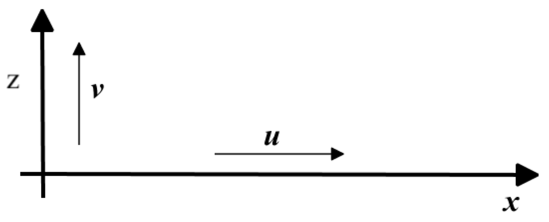
Figure 2.
(a) The shape functions of the salinity equation Equation (15). The black and blue curves are for real part of the solution for the numerical parameters sets of and of for the parameters of . The third red curve shows the imaginary part for the parameters of . (b) Shows the projection of the real part of salinity distribution for , with the parameters of respectively.
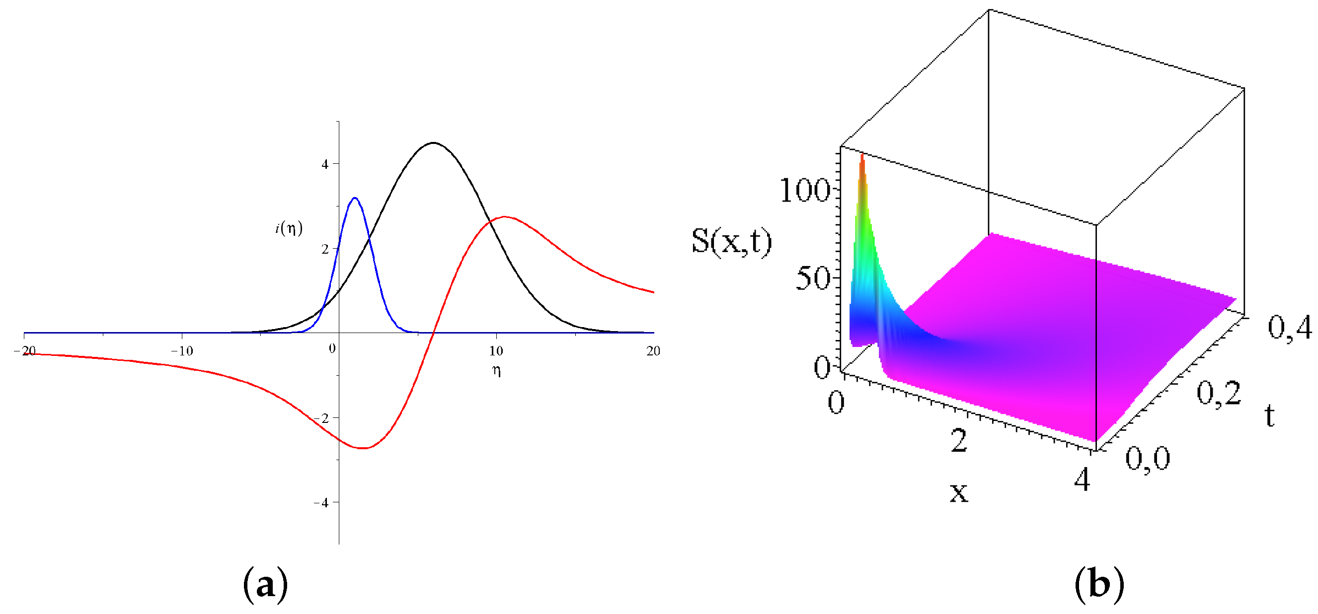
Figure 3.
(a) Two shape functions of the velocity equation Equation (17). The common parameters are are . The black and the blue curves have different values of the parameters namely , and , respectively. (b) The velocity distribution with the parameters of the black curve, respectively.
Figure 3.
(a) Two shape functions of the velocity equation Equation (17). The common parameters are are . The black and the blue curves have different values of the parameters namely , and , respectively. (b) The velocity distribution with the parameters of the black curve, respectively.
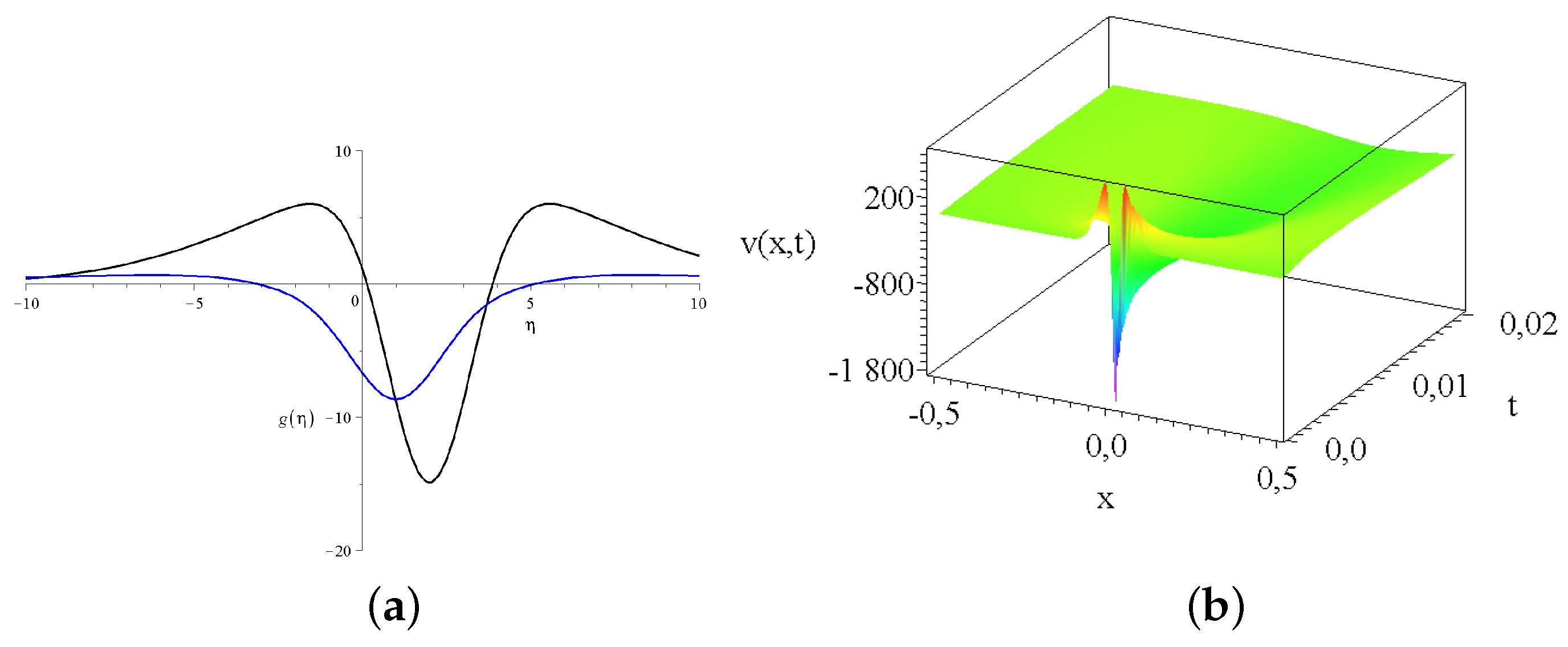
Figure 4.
A possible velocity distribution as a linear combination of three real solutions in the form of , where are . The physical parameters are the same as in Figure 3b). The linear combination parameters s are respectively.
Figure 4.
A possible velocity distribution as a linear combination of three real solutions in the form of , where are . The physical parameters are the same as in Figure 3b). The linear combination parameters s are respectively.
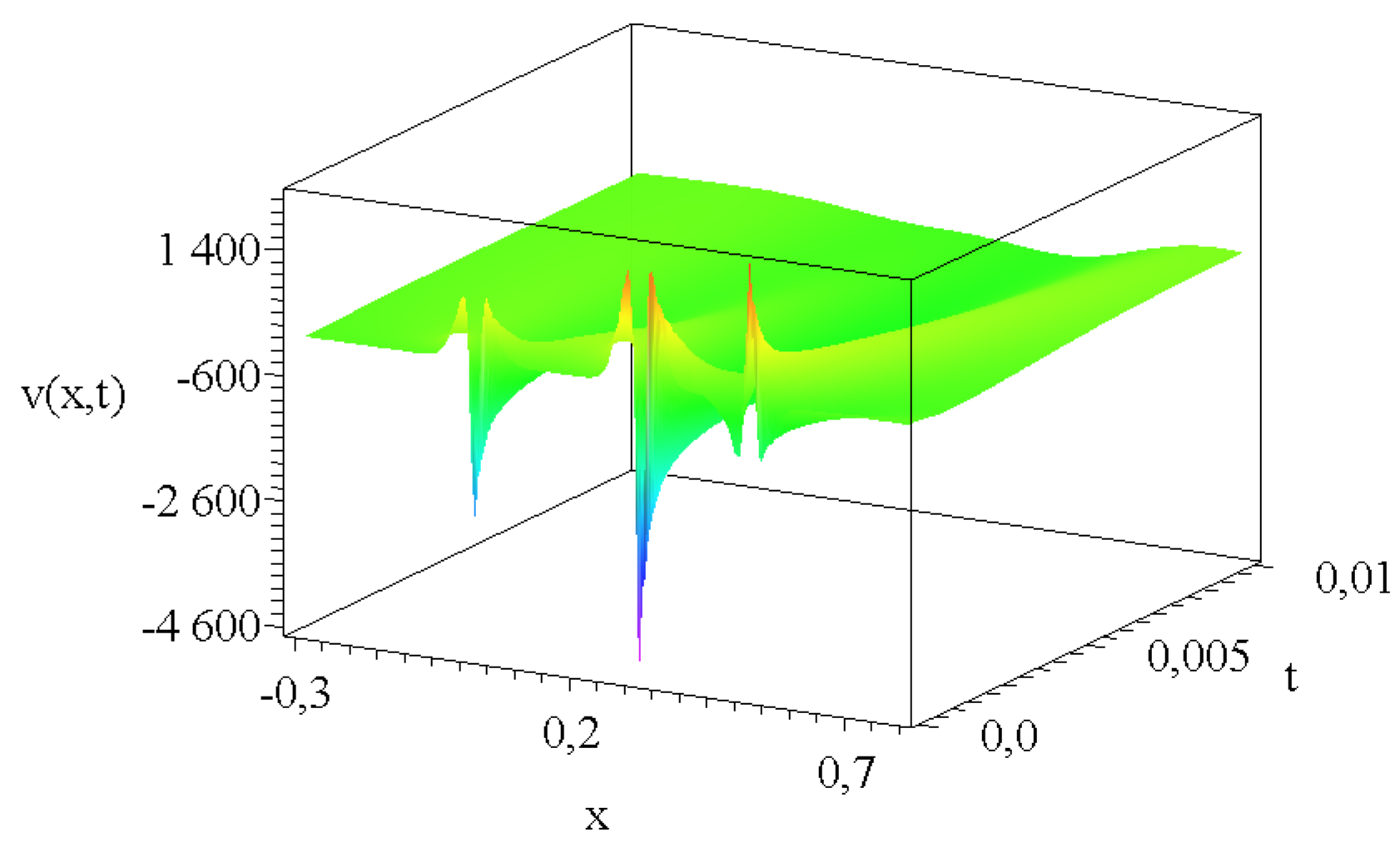
Figure 5.
(a) The Kummer’s M part of the shape functions of the temperature Equation (20). The common parameters are and . The black, blue, red, green, pink, brown, cyan, gray lines are for numerical values of the source strength parameter d of . (b) The real part of the Kummer’s U part with the same parameters.
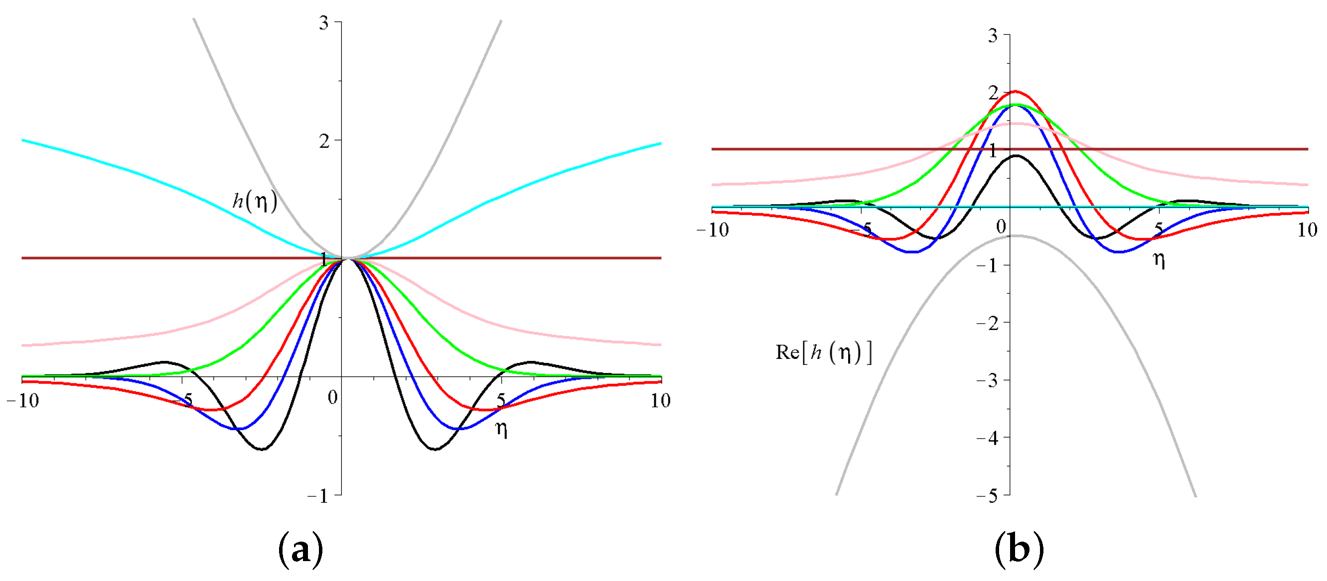
Figure 6.
The Kummer’s M part of the temperature distribution. The three figures from left to right have the source strength of the common parameters are , respectively.
Figure 6.
The Kummer’s M part of the temperature distribution. The three figures from left to right have the source strength of the common parameters are , respectively.
Disclaimer/Publisher’s Note: The statements, opinions and data contained in all publications are solely those of the individual author(s) and contributor(s) and not of MDPI and/or the editor(s). MDPI and/or the editor(s) disclaim responsibility for any injury to people or property resulting from any ideas, methods, instructions or products referred to in the content. |
© 2025 by the authors. Licensee MDPI, Basel, Switzerland. This article is an open access article distributed under the terms and conditions of the Creative Commons Attribution (CC BY) license (http://creativecommons.org/licenses/by/4.0/).
Copyright: This open access article is published under a Creative Commons CC BY 4.0 license, which permit the free download, distribution, and reuse, provided that the author and preprint are cited in any reuse.


