
Submitted:
12 May 2025
Posted:
12 May 2025
You are already at the latest version
Abstract
P91 is a heat-resistant steel widely used in supercritical power plants due to its energy efficiency and environmental benefits. The analysis of the composition distribution of P91 holds profound significance. The Spark Mapping Analysis for Large Samples (SMALS) is an instrument for obtaining high-resolution continuous compositional information on a meter scale. The instrument was employed to scan the entire surface of large samples and provide the elemental composition distribution for P91 steel. Steel sample A was analyzed to establish the partition statistics method for the elements Si, Mn, Cr, Ni, Mo, and Cu. This method was subsequently applied to samples B1, B2, C1, and C2. The partition statistics method can determine the location of segregation and positive and negative segregation areas, which is crucial for studying steel properties and eliminating segregation defects. The degrees of positive and negative segregation were assessed using the upper limit, and the statistical fitting degree of the samples was evaluated based on the 95% criterion. The research indicates that the element content in the positive segregation area fluctuated less and had a lower standard deviation compared to that in the negative segregation area. This method offers valuable guidance for reducing segregation in the production process.
Keywords:
composition distribution
; partition analysis
; P91 steel
; segregation
; SMALS
1. Introduction
Improving thermal power generation technology is one of the essential means to optimize the energy structure and achieve energy saving and emission reduction [1]. The thinning of the central steam pipe wall thickness and high-temperature reheat steam pipe will play a key role in saving resources. P91 steel [2,3] has good high-temperature durability which has a wide range of applications as a high-temperature and high-pressure heat-resistant steel material. It is widely used in sub-critical and super-critical thermal power generation units [4] of the main steam pipe and high-temperature reheat steam pipe, showing excellent overall performance. For large steel ingots, in terms of mechanical properties and physical properties, segregation can make great differences in steel, and even anisotropy, reduce metal yield, endanger product performance, affect the effective use and service life of steel products, and cause hidden dangers [5]. Therefore, the analysis of the composition distribution of P91 steel pipe is beneficial to solve the problems such as creep damage, pinhole cracks, and thermal fatigue damage on the inner surface of the high-temperature components in service.
It is easy to produce selective crystallization, resulting in solute precipitation at the solidification front. When the concentration of the elements in the steel increases, and the element's content does not appear to be fully diffused in the liquid phase, it will form a high concentration of precipitation layer at the solidification front, thus causing segregation. Most of the steel composition segregation distribution is sampled by multi-hole drilling and investigated by Inductively Coupled Plasma Optical Emission Spectrometer(ICP-OES) etc. [6]. ICP has a high detection limit for steel samples, but for large samples it requires multiple holes to be drilled at specific locations and chemically dissolved, which is a huge amount of work and does not accurately reflect the distribution of components on the surface of steel samples. Meanwhile, the method is cumbersome over a long period and not suitable for the distribution of the C element [7]. However, the content of C in steel samples largely determines the properties of steel samples such as strength, plasticity and toughness, so it is essential to analyze the full range of C elements. As a result of not requiring morphology and processing, Laser-Induced Breakdown Spectroscopy [8] (LIBS) has substantial advantages in compositional distribution analysis; Lukas Quackatz et al. [9] visualized the chemical distribution of corroded surfaces of duplex steel with LIBS. They compared the results with conventional measurement methods such as X-ray energy dispersive analysis (EDS) to verify the accuracy of LIBS results, Kazuhiro Kimura et al. [10] measured texture directly in the cross-section of boiler tubes by X-ray diffraction (XRD) and observed that surface on steel has an effect on the macroscopic segregation of steel, and the improvement of macroscopic segregation contributes to the creep strength, and XRD enables nondestructive testing of steel, LIBS has limitations in metal analysis because it is less reproducible and more affected by matrix and self-absorption effects; Micro-beam X-ray fluorescence (μ-XRF) technique is an essential tool for detecting the elemental composition of steel without damage to the sample. Sheng [11] conducted studies on steel samples for high-speed railway axles using the SMALS technique, compared the results with the μ-XRF, and found that, for high-content elements, the two results were similar; for low-content elements, the accuracy of Spark Mapping Analysis for Large Samples (SMALS) precision was better. XRF can analyze samples up to 200 mm long and has a low sensitivity for the analysis of the element Al, so it has some limitations for the analysis of metallic elements. In conclusion, there is no suitable and efficient analytical method for large steel castings, and conventional analytical methods require the samples to be cut and divided into appropriate sizes, making it impossible to analyze the complete components.
SMALS effectively addresses the existing gap in the field of large metal analysis. With its unique three - in - one experimental approach of automatic component processing, precise scanning and positioning, and quantitative spectral analysis, the instrument offers robust support for large - size samples and repeat testing.
Notable progress has been made in developing highly stable and reliable spark excitation light source technology. In this study, we introduced a single - spark integral delay controllable technology, which has a step size adjustment capability of up to 0.4μs. Moreover, a high - precision single - spark spectrum acquisition system was developed. This system not only improved the signal - to - noise ratio but also lowered the detection limit of instrumental analyses.
Figure 1 presents a schematic diagram of a single spark light source. The self - developed high - stability continuous discharge spark light source delivered outstanding performance, with the ability to operate continuously for over 17 hours, reaching the current leading level in this field.
It is worth highlighting that the single spark light source represents a significant advancement and innovation based on the traditional light source. This enables the spark light source to better analyze the elemental composition distribution of large - size samples over an extended period. Unlike the traditional light source, the single spark light source eliminates the need for pre - ignition and does not alter the material surface state, thus preserving the fundamental acquisition of the original state of the material information. The single - spark light source avoids the signal distortion typically associated with pre - ignition. Unlike conventional light sources, it, combined with continuous excitation and high - speed acquisition technology, allows for the collection of a large amount of data in one go, thereby greatly boosting analysis speed and shortening the analysis cycle.
When paired with a precision positioning system, the single - spark light source enables more accurate identification of material defect locations. By analyzing numerous single - discharge signals, it offers detailed insights into the material's elemental distribution, facilitating a more thorough evaluation of material homogeneity.
The single - spark light source can scan extensive material areas, yielding more inclusion - related information and more representative analysis results. In contrast, conventional light sources may only analyze limited areas, making it hard to grasp the overall inclusion distribution.
It addresses issues in characterizing large - metal components like high - speed - train wheels and axles, aircraft - engine turbine - disc blanks, and nuclear/ultra - supercritical - thermal - power - plant pipelines regarding compositional - segregation and inclusion levels across the entire area.
Moreover, the instrument has achieved key technological breakthroughs in the following aspects:
(1) Breakthroughs in the technical problems of highly stable precision optical systems. Optical system stability is improved by designing a low volume thermostat optical system with non-vacuum tidal inert gas filling and deoxygenation technology.
(2) The first international integrated control technology for precision positioning and high-precision spectral scanning and inspection of large-size metal component surfaces without water and air-cooled machining.
(3) The first inverted excitation precision spectrometer and supporting technology in the world. The innovative design of inverted excitation system solves the problem of ash accumulation on the spark table caused by the increase in the number of excitation of the traditional spectrometer. Timed automatic electrode cleaning system realizes dynamic cleaning of the excitation electrode, which ensures the stability of the excitation parameters.
(4) Developed rapid acquisition and processing techniques for massive billions of spectral data. Through the parallel GPU mass data calculation mode, the collection and calculation efficiency are greatly improved, solving the problem of high-speed collection and processing of high-precision big data spectra.
(5) Establishment of statistical characterization methods and models for large scale range compositional segregation. Mathematical models and application standards for compositional analysis and segregation analysis of large-scale metal components such as high-speed railway axles, nuclear power tubes and aero-engine turbine disc forgings have been established.
The successful development of the large-scale metal component compositional segregation analyzer has strongly supported the quality improvement and service performance evaluation of core components of major equipment, and has become an important high-throughput characterization technology for material genetic engineering to support material modification and process optimization as well as quality evaluation. The instrument is the first of its kind in the world, filling the domestic and international technological gaps in the characterization of ultra-large-scale material compositional segregation and inclusions, and greatly enhancing the quality control level and reliability of large metal components. It provides an important technical support for casting of great powers.
Based on the development and research of this instrument, we are expanding the application and have established a partitioning and statistical method to divide the macro-partitioned areas and analyze the characteristic areas of large components. We have also established a statistical method to divide the macro-segregation area of large-size components and to analyze the characteristic area. In this paper, the SMALS was used to analyze P91 steel pipe sample A to establish the partition analysis method, and then the method was applied to P91 billets and pipes from samples B1, B2, C1, and C2. The solidification process of steel produces positive and negative segregation of elements, and for steel samples there are standards that specify the range of elemental melting values to ensure that the melting process, so for the maximum positive and negative segregation of selected steel elemental segregation zones, there must be an upper limit of the maximum segregation of different steel grades to determine the degree of conformity of the steel, i.e. the upper limit of segregation degree .The upper limit of segregation degree of heat-resistant steel was evaluated by Zhang [12]; the equation (1) was as follows, C is the element content in percentage:
When samples were examined by SMALS, a large amount of data was collected from the scanning area. The positive segregation degree and negative segregation degree of the sample were calculated by equations (2) and (3) as follows, in which C97.5% and C2.5% were the content in normal distribution at the right and left sides for 95% confident level. is general mean content.
2. Materials and Methods
2.1. Equipment
The Schematic illustration of SMALS is shown in Figure 2 with the maximum sample size in length × width (1000 mm×500 mm). The sample surface was milled by a vertical numerical control machine prior to scanning. Vertical machining system is to be scanned and analyzed samples are placed on the sample stage with a maximum bearing weight of 900Kg, which can be achieved by placing the samples on the surface of the sample stage, and then the instrument processing center adopts vertical machining center to carry out Z-axis direction of milling on the sample surface. The sample was scanned and excited by a digital spark source along the X-axis at a speed of 1 mm/s. The milling process was cooled by compressed air with water and oil filtration. The milling speed was 500 r/min, the feed rate was 300 mm/min, the milling depth was 0.1mm, the parallelism of the X-axis and the Y-axis was 0.01mm, and the roughness Ra<3.2 um. The instrument is the first to integrate the historical processing system with the spark detection system, which seamlessly connects sample processing with analysis and measurement, free of handling, secondary contamination, and secondary positioning, and realizes the three-in-one characterization test of automatic processing of components, accurate scanning and positioning, and quantitative analysis of spectra.
The Spark Mapping Analysis for Large Samples (SMALS) is an instrument for obtaining high-resolution continuous compositional information on a meter scale. SMALS consists of six systems: the fully automated sample processing system, the Roland Park optical system, the spark light source system, the laser light source system, the stacked grating system, and the data processing system. The SMALS system workflow is shown in Figure 3.
Once the sample has been processed, it is time to set up the parameters and scanning method. The Paschen-Runge Optical System's Photomultiplier Tube (PMT) detector with a wavelength range of 160-650 nm is used to scan and excite the sample with an all-digital, solid-state spark light source. After positioning the sample stage and the spark stage, the motion of the sample stage and the distance of the spark stage inverted on the sample surface were set. According to several experimental tests, it was found that controlling the distance between the spark table and the sample at 0.04 mm was the best for excitation. After the positioning is completed, the control software automatically edits the motion test G code and sends the test command, the electrode material of the spark light source excites a single spark, and the processed sample is scanned and tested, the sample scanning mode can be designed through the scanning coordinates of different sample shapes, and the instrument adopts the horizontal pre-ignition and scanning along the X-axis, and the first point of pre-ignition is 4s at the beginning of each line of scanning when the instrument's spark table is in contact with the surface of the sample. At the beginning of each line of scanning, the first point of contact between the instrument spark table and the sample surface is pre-ignited for 4s, so that the spark scanning excitation effect is stable, and after the pre-ignition, spark excitation scanning is carried out on the surface of the sample at a scanning speed of 1mm/s. The instrument scans the sample one by one at a width of 4mm, so as to realize the analysis and detection of the large samples by scanning the whole area from left to right and from top to bottom.
After the excitation of the beam obtained by the spectroscopic system to obtain multi-element spectra, the acquisition system at the same time to collect the spectral intensity signals detected by the PMT, intensity signals through the acquisition system to return to the computer, the software analysis of the intensity signals into concentration signals, as in Figure 1, the signal conversion is through the intensity ratio of the concentration ratio of the relationship between the formula for conversion, as in equation (4 )[13]:
2.2. Samples
P91 series samples are shown in Figure 4; A is a series steel sample from one factory to establish the partition analysis method; B1, B2, C1, and C2 are steel samples from another factory to verify and apply the partition analysis method, and four samples from the same batch. B1 and B2 were cut from billet B, C1 and C2 were cut from seamless steel pipe C, steel pipe C is made of billet B rolled through piercing. Sample A has an outer diameter of 358 mm and an inner diameter of 242 mm; A1 is a part of A with a size in Length×Width(34mm×20mm). Sample B1 and sample B2 are the top and bottom steel round billets with a diameter of 388 mm, samples C1 and C2 are the top and bottom rings with a diameter of 388 mm intercepted by steel pipe, and five samples were scanned and examined by SMALS. Table 1 shows the sample specific information. Sample specifications for rings are expressed as outer diameter (OD) × inner diameter (ID) × thickness (T); sample specifications for billets are expressed as ϕ (diameter).
2.3. Calibration Curve
As shown in Table 2, more than 20 Certified Reference Materials (CRM) of stainless steel were used in calibration. The spectral lines of Si, Mn, Cr, Ni, Mo and Cu were 212.41nm, 293.30nm, 267.71nm, 218.49nm, 281.61nm, and 233.01nm, respectively. All CRMs were ground by SiC sandpaper in 60 mesh. The R2 of all elements was greater than 0.99.
2.4. Partition Analysis Method
The sample was scanned from left to right along the X-axis direction. The edge of the inner and outer ring was 10 mm and 14 mm without excitation for sample A, C1, and C2; the margin of the outer for round billets was 14 mm for sample B1 and B2; The metallurgical products in cross-section or longitudinal section exhibits symmetry. In the process of steel solidification[14], the location and degree of segregation have relied on the colling rate during solidification and each element's characteristics. The segregation in the symmetry part is also symmetrical, so for the cross-section of round billet or steel pipe, the boundary of the segregation area was evaluated with multiple ring partitions from the inner edge of the ring to the outer edge, and the final partition of segregation analysis was carried out, which was an effective analysis method for the segregation evaluation of large-size metal samples. The partition statistics method is established by using A as an example of a statistical method and then applied to B1, B2, C1, and C2. Based on the established method, the other samples can be examined.
The steps of the partition analysis method are as follows:
Measuring the shape and size of steel samples and completing the excitation scanning by SMALS.
Setting the partition statistics gradients of round sample and name these areas as area Ⅰ, area Ⅱ, area Ⅲ, etc., along the center of the circle toward the outer edge.
Collecting the data of the analyzed area after setting the gradient and evaluating the boundary of the segregation according to the trend of the area mean concentration,
Evaluating the degree of segregation with the upper limit and the statistical fitting degree by the 95% criterion.
The segregation [15] is classified according to the deviation of the original average alloy concentration from the solute concentration in each alloy part, where is positive segregation and is negative segregation. After the samples have been scanned, the total average value of the whole samples is calibrated to the average of their actual content. Therefore, for samples with a constant general average value, when macroscopic segregation occurs in the samples, the contents of different segregation areas are different and always shows a complementary trend between high and low contents.
3. Results and Discussion
This section may be divided by subheadings. It should provide a concise and precise description of the experimental results, their interpretation, as well as the experimental conclusions that can be drawn.
3.1. The Fluctuation Effect on the Different Scanning Areas
In sample A1, different scan area widths of approximately 1mm, 5mm, 10mm, 15mm and 20mm are selected, all of which have an area length of 34mm. The scanning is continuously fired at a rate of 1mm/s and has 125 firing points data per square millimeter. Therefore, as the width of the selection area increases, the amount of data will increase, each area was divided into 34 sub-areas and its average content calculated independently, as in Figure 5(A). For areas of 1mm, 5mm, 10mm, 15mm and 20mm width, the amount of data in the 34 segmented areas is 125, 625, 1250, 1875 and 2500 data points respectively. It can be seen that if we want to analyze the distribution of elemental composition of the whole part, only a small part is not representative, so we choose to use the overall partition statistics method, not only can take into account the location of the sample in each direction, but also for the solidification process of the metal to provide certain recommendations and references. The six elements of Si, Mn, Cr, Ni, Mo, and Cu were statistically analyzed. Observe the fluctuation of the mean content of each sub-area under different area widths. As the area width increases, the content fluctuations of the different area widths gradually decrease around the general mean content for each element.
As in Figure 5(B), the statistical analysis of the relative standard deviation in different area widths shows that as the area width increases, the area relative standard deviation gradually decreases. The above analysis indicates that as the area width increases, some smaller systematic errors can be accommodated for the study of the macroscopic segregation distribution. The analysis of elemental segregation is somewhat different at different scales. When analyzing large samples, we change the previous method of selecting a small area for analysis and divide the sample directly into a circular area from the inside out, which ensures the stability and accuracy of the macro area segregation to the greatest extent possible. For the study of macroscopic segregation of large-size samples, whether it is a steel pipe or ingot, the central element-rich or barren area will have a certain distance from the sample boundary, in order to ensure the accuracy of the curve and reduce the number of regional division of the regional width of the problem, in the regional division of the initial samples for the division of the ten regions, and then based on the element-rich and element-poor Afterwards, according to the element-rich and element-poor intersection area, the area width is finally determined to be more reasonable for macro segregation. The rules for the division of the area are different between rings and billets, because the element-enriched area is obviously narrower after the perforation of the ring, so the width of the area should be smaller as well. So, the establishment of the partition statistics method for large-meter-size samples is of great significance in the analysis of the composition distribution.
3.2. Data Collection and Analysis of Complete Samples
Figure 6 (A) is the physical picture of scanning sample A. As in Figure6 (B), (a1), (b1), (c1), (d1), (e1), and (f1) are to draw the scanned data at equal distances of 3 mm from the center of the ring to the outer edge, and finally to divide it into 11 areas; (a2), (b2), (c2), (d2), (e2), (f2) are the average values of the different elements counted in the 11 independent areas, the horizontal coordinates represent areas divided by the same width and the vertical coordinates represent the average elemental content of each area.; (a3), (b3), (c3), (d3), (e3), (f3) are the final partition areas determined by the comparative statistics between the area mean content and the general mean content. According to Figure6 (B), (a2), (b2), (c2), (d2), (e2), (f2), most of the inflection points for the six elements are in the second and ninth areas, so sample A was divided into 6 mm-20 mm-8 mm and elements Si, Mn, Cr, Ni, Mo, and Cu have a similar diffusion trend. It can be seen that Si, Mn, Cr, Mo, Ni, and Cu are divided into three areas along the inner edge to the outer edge; element Si, Mn, Cr, Mo, and Ni show a negative-positive-negative trend of segregation, element Cu shows a positive-negative-positive trend. This is because heat dissipation is faster at the edges than inside, and a temperature gradient[16] is formed in the ingot for element content. The element content is carried out separately throughout section but from the outer edge of the ingot and the mold. The cooling rate at the edge is faster than in the inner part of the ring. The element content that cannot be fully diffused in the liquid phase will form a higher or lower segregation area.
In the process of macroscopic segregation, the liquid phase flow between the dendritic crystals is opposite to the solidification speed, resulting in negative segregation, for the Cu element, its melting point is 1083 ℃, and Si, Mn, Cr, Ni, Mo elements of the melting point of 1414 ℃, 1246 ℃, 1907 ℃, 1455 ℃, 2623 ℃, the casting center of the region is enriched in the low-melting element of the liquid, due to the casting solidification occurs when the shrinkage and between the dendritic crystals to form cavities (here for the negative pressure), coupled with the temperature drop, so that the gas precipitation in the liquid and the formation of pressure, the casting center of the low-melting elements of the liquid concentration of higher along the columnar crystals of the "channel" between the casting of the outer layer of pressure. In the circle steel samples, the areas with more positive and negative segregation defects were better delineated, which is instructive for the separate analysis of the positive and negative segregation areas in the full-size steel samples.
Table 3 is a statistic table of component segregation of different areas in sample A. The positive and negative segregation areas, area mean content, positive segregation degree, negative segregation degree, statistical fitting degree, and standard deviation of different elements are counted.
The statistical fitting degree is the ratio of the position content in the specification range to the total content of all positions in the analyzed area [12]. All data outliers were evaluated according to the 95% fitting degree criteria because the confidence level in the chemical analysis was usually at 95% confidence degree, so the statistical fitting degree should be at least 95%. According to Table 3, it was found that the statistical fitting degree of all areas for sample A was greater than 95%. The positive and negative segregation degree of the steel samples did not exceed the upper limit Ds(max) for all areas of all elements, except for the positive segregation degree D(+) of element Cr in areas Ⅰ. The element content standard deviation and segregation were lower in the area, and is average value was higher than the general average for sample A. This is due to the fact that the elemental composition in the negative segregation areas does not diffuse uniformly. The excessive differences between the high and low elemental compositions were shown in the negative segregation areas. Thus, the element-enriched positive segregation area is more uniform.
3.3. The Fluctuation Effect on the Different Scanning Areas
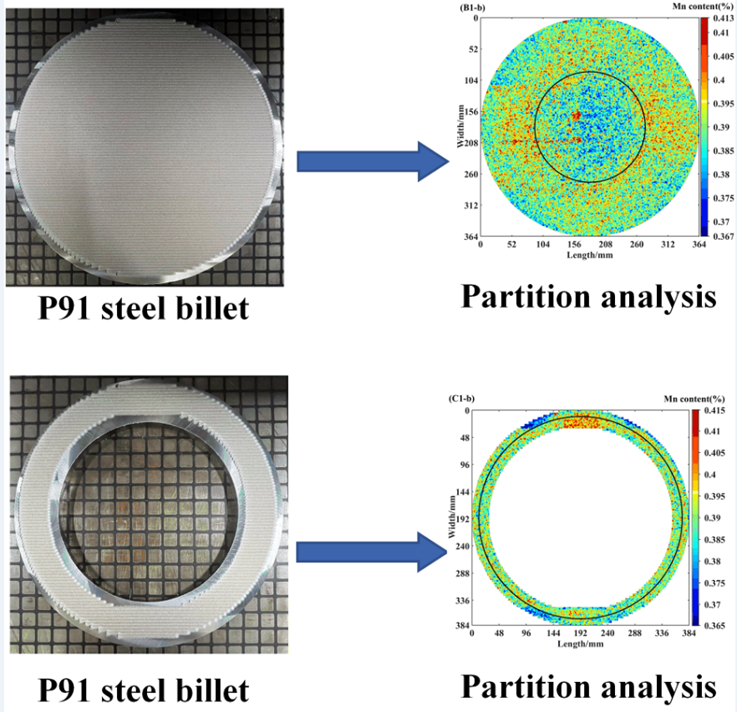
The method of partition statistics can be applied not only to rings but also to round billets. Also, measures are taken starting from the inner center and approaching the outer edge to determine the segregation area. Figure 7(A), (B1), (C1), (B2), and (C2) show the scanned physical images of the top round billet, the top ring, the bottom round billet, and the bottom ring for super-critical power steel.
Figure 7(B) shows the two-dimensional plots of Mn elemental contents about the partitioning process and partitioning completion in the four samples. Take the Mn element as an example: the partition statistics of each sample are set to the same gradient, and the partition gradient of the billet was set to 10 mm, which could be divided into 19 areas, as shown in Figure 7(B)(B1-a) and Figure 7(B) (B2-a); The ring sample was a part of the finished steel pipe, and the 3 mm excitation area of the scan was divided into ten areas, as shown in Figure 7(B) (C1-a) and Figure 7(B) (C2-a).
According to this partitioning gradient, Figure 7(C), (B1), (B2), (C1), and (C2) shows the statistical graphs of the average content of each area of elements Si, Mn, Cr, Ni, Mo, and Cu in the four samples. The top sample B1 and the bottom sample B2 of the round billet show that most of the elements start to rise above the total average or fall below the total average around the ninth area; the top ring C1 and the bottom ring C2 show that most of the elements start to rise above the total average or fall below the total average around the fourth area. Therefore, as in Figure.7B (B1-b) and Figure.7B (B2-b), the samples were divided into two areas from 90 mm to the outer edge of the billet; and as in Figure 7(B) (C1-b) and Figure 7(B) (C2-b), the ring was also divided into two areas from 18 mm to the outer edge.
The content fluctuations of samples B1, B2 were higher than those of C1, C2 because the steel pipe was pierced from the billet. In the piercing process[17], the heating temperature of the billet should be controlled in the best deformation temperature range; the average heating temperature is generally controlled at 1200-1250℃, and then after stress relief annealing, normalizing, tempering, straightening, grinding, and other processes, the final pipe was formed. Therefore, some defects are eliminated during the processing of real steel pipes, so the fluctuations of pipe were relatively minor compared with the billets. From Figure 7(C) (B1) and (B2), it was found that most of the elements had positive and negative segregation separation circles whose half diameter was about 1/2 of the sample half diameter. From Figure 7(C) (C1) and (C2), it was found that most of the elements had positive and negative segregation separation circles at a position close to 2/3 of the sample ring thickness. The partitioning statistics methods of segregation area for round and ring samples were also applicable to other steel samples.
For samples B1 and C1, the area Ⅰ of Si, Mn, Cr, Ni, and Mo was the negative segregation area, and area Ⅱ was the positive segregation area; The Cu element in area Ⅰ was positive segregation, and area Ⅱ was negative segregation. For sample B2, the Cr elements in areas Ⅰ and Ⅱ were uniforms; The area Ⅰ of Si, Mn, Ni, and Mo was positive segregation; the area Ⅱ was negative segregation; The area Ⅰ of the Cu element was the negative segregation, and area Ⅱ was positive segregation. In the bottom ring C2, the area Ⅰ was positive segregation and area Ⅱ was negative segregation for most elements.
Partition statistics were performed for the top round billet B1, the top ring C1, the bottom round billet B2, and the bottom ring C2, and the data are shown in Table 4. For samples B1 and B2, the positive and negative segregation degree was evaluated by the upper limit DS (max). Al elements in sample B1 and B2 did not exceed the upper limit DS (max) in areas I and II, except the segregation degree of Cr in sample B1 was slightly exceeded. As shown in Figure 7(C), the fluctuation of Cr content in sample B1 was higher than that of sample B2. Hence, the positive and negative segregation degrees of B1 were also higher than those of sample B2. It can be seen that the statistical fitting degree of all elements in areas Ⅰ and Ⅱ was satisfied with over 95% requirement. For samples C1 and C2, all elements did not exceed the upper limit DS (max) in areas I and II, except the segregation degree of Cr in sample C2 and Mo in sample C1 were slightly exceeded. It can be seen that the statistical fitting degree of all elements in area Ⅰ and Ⅱ was satisfied with over 95% requirement, except the element Mo in sample C1. Table 4 shows that the element content standard deviation and segregation were lower in the area where the average value was higher than the general average for sample P91.
4. Conclusions
This paper comprehensively elucidates the structure, workflow, and innovative aspects of the SMALS instrument. Our primary objective is to advance the application of SMALS in large - scale sample analysis through the development of a partition analysis method grounded in statistical approaches. The development and application of the regional analysis method to P91 steel, including billets and rings, enables the SMALS technique to extract and analyze area data from the entire scanned compositional distribution. This method allows for direct comparison and individual analysis of regional versus global characteristics. Moreover, it facilitates targeted selection of feature areas within the entire composition distribution. It aims to deepen the comprehension and underscore the significance of sample analysis methodologies, thereby contributing to the broader field of materials characterization.
(1) The rule of partition statistics is based on comparing the area mean content with the general mean content, the area means lower than the general mean belongs to one area and the area mean higher belongs to another. The positive and negative segregation areas of the steel samples are clearly separated by the partition method. With sample A, the partition statistics method was established to determine the segregation areas, and the positive and negative segregation degree and the statistical conformity degree were examined for large samples, the distribution of elements can be seen from a macro perspective, which is more comprehensive than the analysis of small areas.
(2) The partitioning statistics method was applied to the round billets and pipe rings. The round billets were divided into inner and outer areas, and the outer area was 90 mm from the center of the circle; the pipe rings were divided into two areas, and the outer area was 18 mm from the center of the circle. The partition statistics showed that the elemental content distribution of the round billets and rings had similar trends, the segregation of the pipe rings was improved after the piercing process of the round billet, the elemental content distribution was less fluctuated, and the finished pipes were more homogeneous than the round billets.
(3) The Spark Mapping Analysis for Large Samples (SMALS) technique was used to scan the entire large sample surface and the elemental composition distribution for P91 steel was given. It was found that the standard deviation of element content and segregation was lower in the area where the average value was higher than the general average for the same P91 pipe. This means that the variation in content was less in the element rich areas than in the element poor areas. During solidification, due to the different melting points of the elements, the low melting point element Cu showed an opposite diffusion trend to the other elements during solute diffusion.
Author Contributions
B.L.: conceptualization, writing– original draft , writing– review & editing, investigation; L.Z.: Investigation and review; L.S.: investigation; J.Y.: investigation, writing– review & editing; L.Y.: writing– review & editing; L.Y.: methodology ; Q.Z.: investigation and software ; H.W.: Conceptualization, Methodology, ; Y.J.: investigation, methodology, Writing– original draft, Writing– review & editing. All authors have read and agreed to the published version of the manuscript.
Funding
This research was funded by the National Key Research and Development Program of China (No. 2023YFB3712102) and National Key Platform for New Materials - New Material Testing and Assessment (TC230H0A7).
Data Availability Statement
The original contributions presented in this study are included in the article. Further inquiries can be directed to the corresponding authors.
Conflicts of Interest
The authors have no conflicts to disclose.
References
- Rerak, M.; Ocłoń, P. Thermal Analysis of Underground Power Cable System. J. Therm. Sci. 2017, 26, 465–471. [CrossRef]
- Pandey, C.; Mahapatra, M.M.; Kumar, P.; Saini, N. Some Studies on P91 Steel and Their Weldments. Journal of Alloys and Compounds 2018, 743, 332–364. [CrossRef]
- Han, K.; Ding, H.; Fan, X.; Li, W.; Lv, Y.; Feng, Y. Study of the Creep Cavitation Behavior of P91 Steel under Different Stress States and Its Effect on High-Temperature Creep Properties. Journal of Materials Research and Technology 2022, 20, 47–59. [CrossRef]
- Maddi, L.; Ballal, A.R.; Peshwe, D.R.; Mathew, M.D. Influence of Normalizing and Tempering Temperatures on the Creep Properties of P92 Steel. High Temperature Materials and Processes 2020, 39, 178–188. [CrossRef]
- Ge, H.; Ren, F.; Li, J.; Hu, Q.; Xia, M.; Li, J. Modelling of Ingot Size Effects on Macrosegregation in Steel Castings. Journal of Materials Processing Technology 2018, 252, 362–369. [CrossRef]
- Zheng, P.; Luo, Y.; Wang, J.; Yang, Y.; Hu, Q.; Mao, X.; Lai, C. Improved Solution Cathode Glow Discharge Micro-Plasma Source with a Geometrically Optimized Stainless Steel Auxiliary Cathode for Optical Emission Spectrometry of Metal Elements. Microchemical Journal 2022, 172, 106883. [CrossRef]
- Adya, V.C.; Sengupta, A.; Thulasidas, S.K.; Natarajan, V. Direct Determination of S and P at Trace Level in Stainless Steel by CCD-Based ICP-AES and EDXRF: A Comparative Study. At.Spectrosc. 2016, 37, 19–24. [CrossRef]
- Liu, R.; Rong, K.; Wang, Z.; Cui, M.; Deguchi, Y.; Tanaka, S.; Yan, J.; Liu, J. Sample Temperature Effect on Steel Measurement Using SP-LIBS and Collinear Long-Short DP-LIBS. ISIJ Int. 2020, 60, 1724–1731. [CrossRef]
- Quackatz, L.; Griesche, A.; Kannengiesser, T. Spatially Resolved EDS, XRF and LIBS Measurements of the Chemical Composition of Duplex Stainless Steel Welds: A Comparison of Methods. Spectrochimica Acta Part B: Atomic Spectroscopy 2022, 193, 106439. [CrossRef]
- Kimura, K.; Kwak, K.; Nambu, S.; Koseki, T. Nondestructive Evaluation of Macro Segregation in Creep Strength Enhanced 9Cr–1Mo–V–Nb Steel. Scripta Materialia 2020, 188, 179–182. [CrossRef]
- Sheng, L.; Yuan, L.; Jia, Y.; Zhao, L.; Zhang, X.; Yu, L.; Zhang, Q.; Wang, H. Full-Scale Spark Mapping of Elements and Inclusions of a High-Speed Train Axle Billet. J. Anal. At. Spectrom. 2022, 37, 1522–1534. [CrossRef]
- Zhang, X.; Jia, Y.; Sheng, L.; Yuan, L.; Li, J. Characterization of Segregation Degree for Large Size Metal Component and Application on High-Speed Train Wheel. Analytica Chimica Acta 2022, 1203, 339719. [CrossRef]
- Wang, H.; Zhao, L.; Jia, Y.; Li, D.; Yang, L.; Lu, Y.; Feng, G.; Wan, W. State-of-the-Art Review of High-Throughput Statistical Spatial-Mapping Characterization Technology and Its Applications. Engineering 2020, 6, 621–636. [CrossRef]
- Li, J.; Xu, X.; Ren, N.; Xia, M.; Li, J. A Review on Prediction of Casting Defects in Steel Ingots: From Macrosegregation to Multi-Defect Model. J. Iron Steel Res. Int. 2022, 29, 1901–1914. [CrossRef]
- Shen, Y.; Yang, S.; Liu, J.; Liu, H.; Zhang, R.; Xu, H.; He, Y. Study on Micro Segregation of High Alloy Fe–Mn–C–Al Steel. steel research int. 2019, 90, 1800546. [CrossRef]
- He, Q.; Wu, H.; Meng, H.; Hu, Z.; Xie, Z. Molten Steel Level Detection by Temperature Gradients With a Neural Network. IEEE Access 2019, 7, 69456–69463. [CrossRef]
- Zhang, Y.; Yi, R.; Wang, P.; Fu, C.; Cai, N.; Ju, J. Self-Piercing Riveting of Hot Stamped Steel and Aluminum Alloy Sheets Base on Local Softening Zone. steel research int. 2021, 92, 2000535. [CrossRef]
Figure 1.
Schematic diagram of single spark light source excitation.
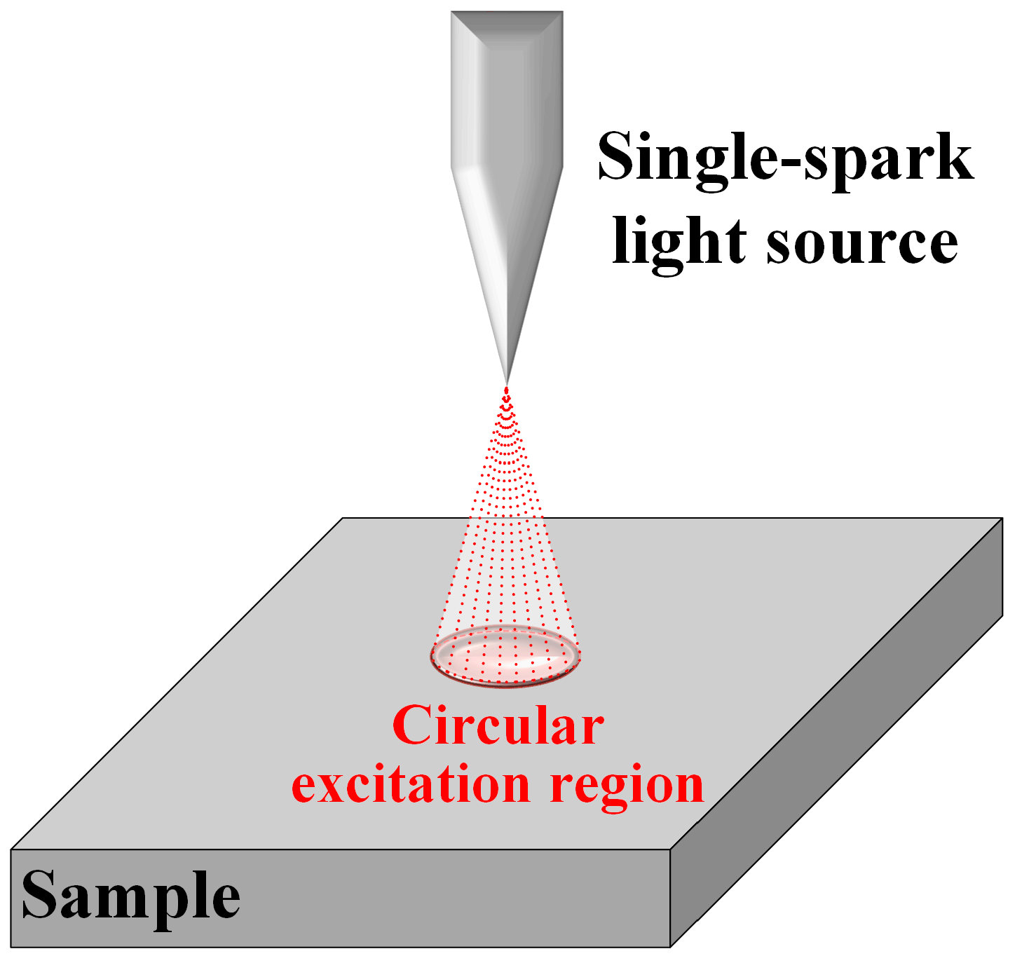
Figure 2.
Schematic setup of the SMALS equipment.
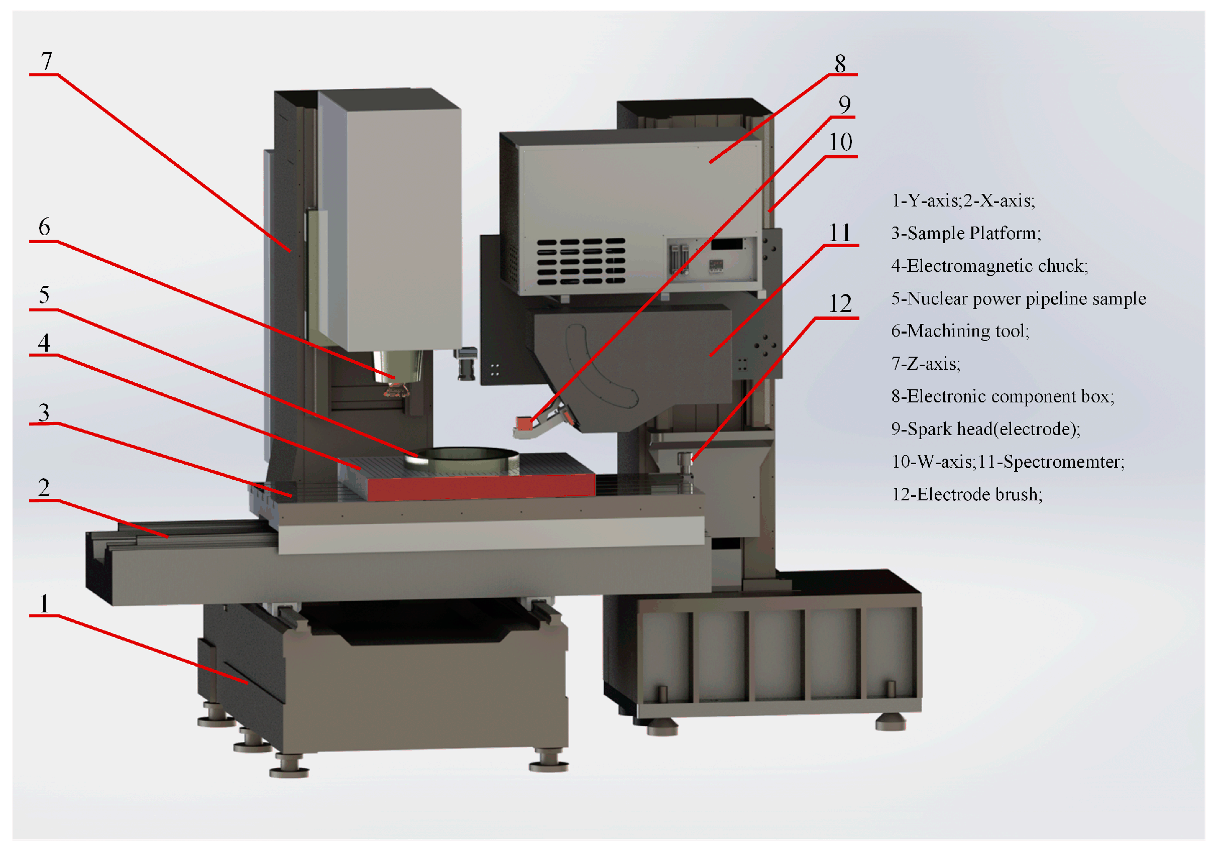
Figure 3.
SMALS system workflow diagram.
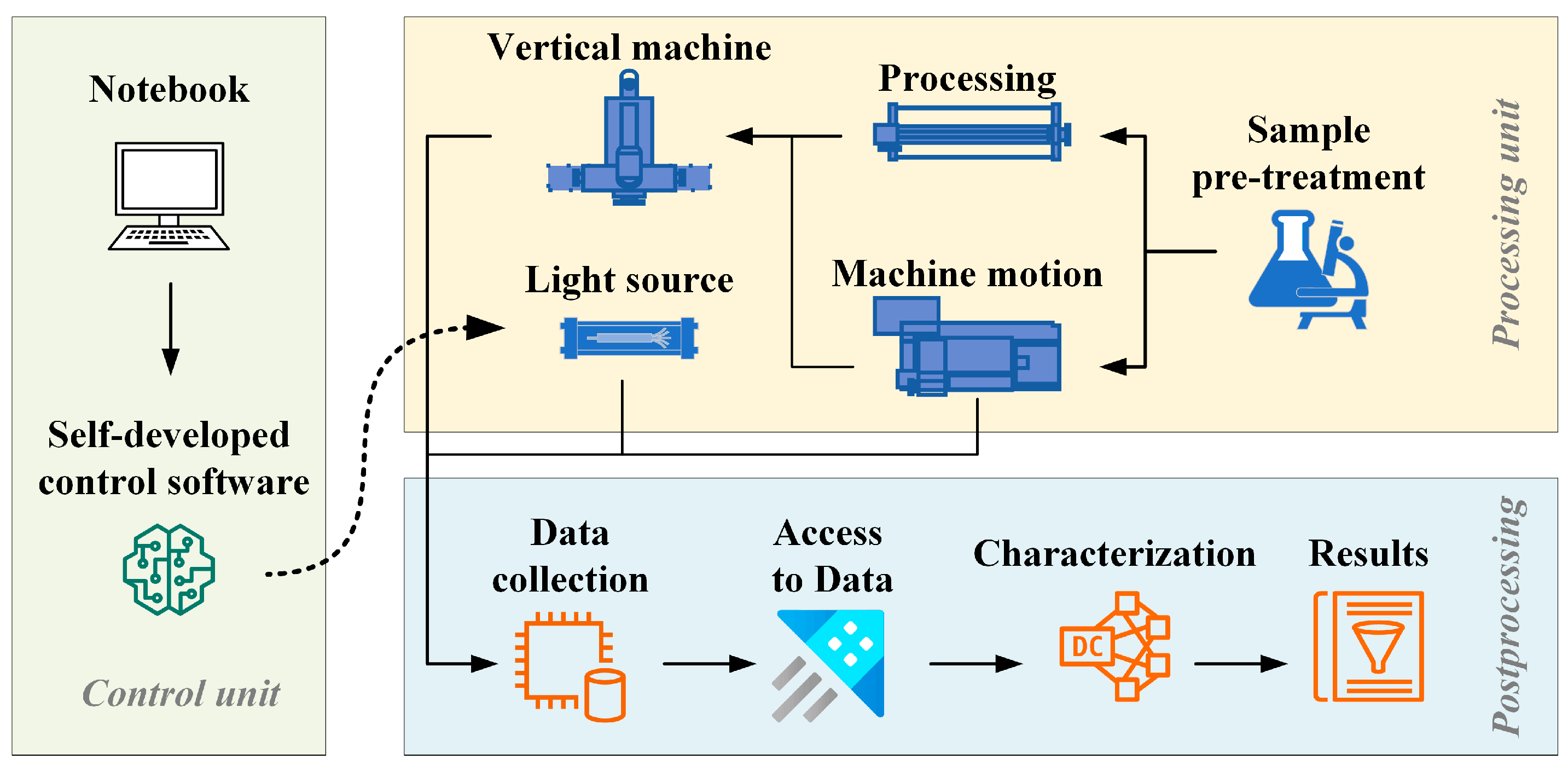
Figure 4.
Schematic diagram of steel samples A, B1, B2, C1, C2.
Figure 5.
(A) Statistical map of the content fluctuations with different area width in (a)Si, (b)Mn, (c)Cr, (d)Ni, €Mo, and (f)Cu. (B) Diagram of relative standard deviation with different area width for elements.
Figure 5.
(A) Statistical map of the content fluctuations with different area width in (a)Si, (b)Mn, (c)Cr, (d)Ni, €Mo, and (f)Cu. (B) Diagram of relative standard deviation with different area width for elements.
Figure 6.
(A) Diagram of Sample A scanned by SMALS. (B) Statistical map of the scanned partition for sample A for the element Si, Mn, Cr, Mo, Ni, and Cu.
Figure 6.
(A) Diagram of Sample A scanned by SMALS. (B) Statistical map of the scanned partition for sample A for the element Si, Mn, Cr, Mo, Ni, and Cu.
Figure 7.
(A) Diagram of the steel samples scanned by SMALS. (B) Elemental segregation map of the Mn element. (C) Statistical map of the scanned partition of the steel sample.
Figure 7.
(A) Diagram of the steel samples scanned by SMALS. (B) Elemental segregation map of the Mn element. (C) Statistical map of the scanned partition of the steel sample.

Table 1.
Sample specification and elemental content.
| Sample | Specification | Elemental content | |||||
| Si | Mn | Cr | Ni | Mo | Cu | ||
| A | 358×242×58 | 0.27 | 0.43 | 8.35 | 0.17 | 0.89 | 0.14 |
| B1 | ϕ388 | 0.30 | 0.39 | 8.54 | 0.14 | 0.93 | 0.035 |
| C1 | 400×300×50 | ||||||
| B2 | ϕ388 | ||||||
| C2 | 400×300×50 | ||||||
Table 2.
Calibration curve of elements Si, Mn, Cr, Ni, Mo, and Cu.
| Element | Spectral lines(nm) | Content range (%) | Calibration curve | R2 |
| Si | 212.41 | 0.103~1.05 | 0.00035 × I2 + 0.027 × I − 0.053 | 0.994 |
| Mn | 293.30 | 0.126~1.96 | 0.010 × I2 + 0.0066 × I − 0.0019 | 0.993 |
| Cr | 267.71 | 7.4~24.1 | 1.39 × I2 − 0.21 × I − 0.000039 | 0.992 |
| Ni | 218.49 | 0.062~1.432 | 0.015 × I2 + 0.010 × I − 0.019 | 0.997 |
| Mo | 281.61 | 0.089~1.01 | −0.015 × I2 + 0.043 × I − 0.011 | 0.991 |
| Cu | 233.01 | 0.061~0.69 | 0.0018 × I2 + 0.0012 × I − 0.00087 | 0.999 |
Table 3.
Statistic table of component segregation of different areas in Sample A.
| Elements | General mean content(%) | Area | Area mean content(%) | DS(-)(%) | DS(+)(%) | DS(max)(%) | Statistical fitting degree(%) | Specification range (%) | Standard deviation(%) |
| Si | 0.27 | Ⅰ | 0.268 | -4.45 | 5.79 | 16.61 | 100.00 | 0.20~0.50 | 0.0080 |
| Ⅱ | 0.271 | -3.55 | 4.62 | 100.00 | 0.0060 | ||||
| Ⅲ | 0.269 | -4.06 | 5.10 | 100.00 | 0.0070 | ||||
| Mn | 0.43 | Ⅰ | 0.427 | -3.76 | 4.24 | 13.47 | 100.00 | 0.30~0.60 | 0.0090 |
| Ⅱ | 0.433 | -2.92 | 3.65 | 100.00 | 0.0080 | ||||
| Ⅲ | 0.427 | -3.61 | 3.65 | 100.00 | 0.0080 | ||||
| Cr | 8.35 | Ⅰ | 8.325 | -3.31 | 3.68 | 3.53 | 98.98 | 8.00~9.50 | 0.15 |
| Ⅱ | 8.381 | -2.93 | 3.18 | 99.89 | 0.13 | ||||
| Ⅲ | 8.309 | -3.45 | 3.39 | 98.26 | 0.15 | ||||
| Ni | 0.17 | Ⅰ | 0.169 | -5.27 | 6.22 | 20.47 | 100.00 | ≤0.40 | 0.0049 |
| Ⅱ | 0.172 | -4.89 | 5.00 | 100.00 | 0.0043 | ||||
| Ⅲ | 0.167 | -8.13 | 5.93 | 100.00 | 0.0057 | ||||
| Mo | 0.89 | Ⅰ | 0.881 | -4.16 | 4.34 | 9.7 | 95.38 | 0.85~1.05 | 0.019 |
| Ⅱ | 0.895 | -3.61 | 4.20 | 99.72 | 0.018 | ||||
| Ⅲ | 0.886 | -3.47 | 3.66 | 98.87 | 0.016 | ||||
| Cu | 0.14 | Ⅰ | 0.141 | -2.65 | 2.81 | 22.34 | 99.98 | ≤0.20 | 0.0031 |
| Ⅱ | 0.140 | -2.48 | 2.43 | 100.00 | 0.0023 | ||||
| Ⅲ | 0.140 | -2.34 | 2.29 | 99.98 | 0.0028 |
Table 4.
This is a table. Tables should be placed in the main text near to the first time they are cited.
Table 4.
This is a table. Tables should be placed in the main text near to the first time they are cited.
| Element | General mean content(%) | Sample | Area | Mean content(%) | DS(-)(%) | DS(+)(%) | DS(max) (%) | Statistical fitting degree(%) | Specification range (%) | Standard deviation (%) |
| Si | 0.3 | B1 | Ⅰ | 0.298 | -3.87 | 6.52 | 15.84 | 99.96 | 0.20~0.40 | 0.0087 |
| Ⅱ | 0.301 | -3.41 | 4.57 | 100.00 | 0.0062 | |||||
| C1 | Ⅰ | 0.298 | -8.95 | 9.59 | 100.00 | 0.014 | ||||
| Ⅱ | 0.302 | -9.31 | 10.90 | 100.00 | 0.015 | |||||
| B2 | Ⅰ | 0.302 | -3.72 | 6.32 | 100.00 | 0.0077 | ||||
| Ⅱ | 0.299 | -3.81 | 6.68 | 99.98 | 0.0084 | |||||
| C2 | Ⅰ | 0.301 | -3.62 | 3.73 | 100.00 | 0.0057 | ||||
| Ⅱ | 0.300 | -4.36 | 4.26 | 99.98 | 0.0074 | |||||
| Mn | 0.39 | B1 | Ⅰ | 0.388 | -3.77 | 4.52 | 14.07 | 100.00 | 0.30~0.50 | 0.0083 |
| Ⅱ | 0.391 | -3.47 | 3.89 | 100.00 | 0.0074 | |||||
| C1 | Ⅰ | 0.392 | -6.99 | 8.35 | 99.99 | 0.015 | ||||
| Ⅱ | 0.392 | -6.99 | 8.35 | 99.99 | 0.015 | |||||
| B2 | Ⅰ | 0.393 | -4.36 | 5.03 | 100.00 | 0.0094 | ||||
| Ⅱ | 0.389 | -4.42 | 5.20 | 99.99 | 0.01 | |||||
| C2 | Ⅰ | 0.391 | -3.78 | 4.10 | 100.00 | 0.0078 | ||||
| Ⅱ | 0.389 | -4.55 | 4.17 | 99.99 | 0.0086 | |||||
| Cr | 8.54 | B1 | Ⅰ | 8.524 | -4.65 | 5.8 | 3.50 | 99.47 | 8.00~9.50 | 0.23 |
| Ⅱ | 8.545 | -4.52 | 5.37 | 99.68 | 0.22 | |||||
| C1 | Ⅰ | 8.540 | -2.11 | 2.35 | 100.00 | 0.097 | ||||
| Ⅱ | 8.539 | -2.07 | 2.33 | 100.00 | 0.096 | |||||
| B2 | Ⅰ | 8.538 | -0.11 | 0.10 | 100.00 | 0.0047 | ||||
| Ⅱ | 8.541 | -0.11 | 0.10 | 100.00 | 0.0051 | |||||
| C2 | Ⅰ | 8.571 | -3.96 | 4.50 | 99.89 | 0.18 | ||||
| Ⅱ | 8.508 | -5.27 | 4.64 | 98.36 | 0.21 | |||||
| Ni | 0.14 | B1 | Ⅰ | 0.141 | -4.57 | 4.66 | 22.34 | 100.00 | 0~0.20 | 0.0033 |
| Ⅱ | 0.140 | -10.05 | 5.99 | 100.00 | 0.0053 | |||||
| C1 | Ⅰ | 0.140 | -3.14 | 3.18 | 100.00 | 0.0023 | ||||
| Ⅱ | 0.140 | -2.95 | 2.97 | 100.00 | 0.0021 | |||||
| B2 | Ⅰ | 0.143 | -11.34 | 12.05 | 100.00 | 0.0085 | ||||
| Ⅱ | 0.139 | -12.09 | 12.49 | 99.99 | 0.0088 | |||||
| C2 | Ⅰ | 0.141 | -7.16 | 9.37 | 100.00 | 0.0059 | ||||
| Ⅱ | 0.139 | -10.63 | 8.56 | 99.99 | 0.0065 | |||||
| Mo | 0.93 | B1 | Ⅰ | 0.917 | -3.22 | 3.82 | 9.51 | 100.00 | 0.85~1.05 | 0.017 |
| Ⅱ | 0.934 | -2.96 | 3.38 | 100.00 | 0.015 | |||||
| C1 | Ⅰ | 0.924 | -11.24 | 11.05 | 91.28 | 0.053 | ||||
| Ⅱ | 0.938 | -12.4 | 13.22 | 89.05 | 0.062 | |||||
| B2 | Ⅰ | 0.938 | -3.25 | 3.33 | 100.00 | 0.016 | ||||
| Ⅱ | 0.927 | -3.09 | 3.50 | 99.99 | 0.016 | |||||
| C2 | Ⅰ | 0.931 | -4.28 | 4.58 | 99.98 | 0.021 | ||||
| Ⅱ | 0.929 | -4.25 | 4.67 | 99.94 | 0.021 | |||||
| Cu | 0.035 | B1 | Ⅰ | 0.0352 | -1.87 | 1.72 | 41.74 | 100.00 | 0~0.10 | 0.00032 |
| Ⅱ | 0.0349 | -2.02 | 1.80 | 100.00 | 0.00034 | |||||
| C1 | Ⅰ | 0.0351 | -4.56 | 4.53 | 100.00 | 0.00082 | ||||
| Ⅱ | 0.0349 | -5.57 | 4.85 | 100.00 | 0.00092 | |||||
| B2 | Ⅰ | 0.0349 | -1.93 | 9.51 | 100.00 | 0.00080 | ||||
| Ⅱ | 0.0350 | -1.85 | 7.43 | 100.00 | 0.00078 | |||||
| C2 | Ⅰ | 0.0350 | -1.26 | 1.24 | 100.00 | 0.00022 | ||||
| Ⅱ | 0.0350 | -1.37 | 1.29 | 100.00 | 0.00024 |
Disclaimer/Publisher’s Note: The statements, opinions and data contained in all publications are solely those of the individual author(s) and contributor(s) and not of MDPI and/or the editor(s). MDPI and/or the editor(s) disclaim responsibility for any injury to people or property resulting from any ideas, methods, instructions or products referred to in the content. |
© 2025 by the authors. Licensee MDPI, Basel, Switzerland. This article is an open access article distributed under the terms and conditions of the Creative Commons Attribution (CC BY) license (http://creativecommons.org/licenses/by/4.0/).
Copyright: This open access article is published under a Creative Commons CC BY 4.0 license, which permit the free download, distribution, and reuse, provided that the author and preprint are cited in any reuse.


