β-Optimization in the Information Bottleneck Framework: A Theoretical Analysis

1. Introduction

In modern representation learning, the Information Bottleneck (IB) principle provides a theoretical framework for extracting a concise yet informative representation of data [1]. Given an input random variable X and a target variable Y, the IB method seeks a “bottleneck” variable Z (the representation) that compresses X while preserving information useful for predicting Y. Formally, Z is chosen to maximize the mutual information $I(Z;Y)$ under a constraint on $I(Z;X)$ [1]. Equivalently, one can solve the Lagrangian formulation introduced by Tishby et al. [1], which defines the IB objective as:

$$\mathcal{L}\left(p\right(z\left|x\right);\beta )=I(Z;Y)-\beta I(Z;X),\mathrm{with}\beta \ge 0,$$

(1)

where $\beta$ is a non-negative Lagrange multiplier controlling the trade-off between the prediction term $I(Z;Y)$ and the compression term $I(Z;X)$. By adjusting $\beta$, one traces out the Pareto-optimal trade-offs between retaining information about Y versus compressing X.

Selecting an optimal $\beta$: In practice, choosing the “right” $\beta$ is non-trivial and has traditionally relied on brute-force search or cross-validation. Tishby et al. [1] initially suggested “sweeping” over $\beta$ to plot the IB curve and then picking an operating point. This trial-and-error approach can be computationally expensive and may fail to capture the subtle trade-offs in complex data. The need for a principled criterion to determine an optimal $\beta$ (denoted ${\beta }^{*}$) — one yielding a representation $Z^{*}$ that achieves a specific kind of optimality in the compression-prediction balance — motivates my work. I ask: How can one characterize and compute ${\beta }^{*}$ theoretically, without resorting solely to empirical tuning?

Recent studies have begun to address this question. Wu et al. (2019) [9] introduced the concept of IB-learnability to provide guidance on choosing $\beta$. They define conditions under which a given $\beta$ will avoid trivial solutions (i.e., Z independent of X) and derive a threshold for $\beta$ (specific to $(X,Y)$) related to the existence of meaningful representations. Independently, Rodríguez Gálvez et al. (2020) [8] analyzed the mapping between $\beta$ and the compression rate, showing that under certain convexity assumptions each point on the IB curve corresponds to a unique $\beta$. These works suggest that an optimal $\beta$ could be identified as a critical value related to the IB curve’s geometry. Moreover, a recent multi-objective perspective treats IB as a bi-objective optimization (maximizing $I(Z;Y)$ and minimizing $I(Z;X)$ jointly) to adaptively find trade-offs without a fixed $\beta$ [12]. Such methods confirm that finding the best balance between compression and prediction is challenging and important.

In deep learning, two notable IB-based paradigms have emerged: the Variational Information Bottleneck (VIB) [5] and what I term the Neural Information Bottleneck (NIB). VIB refers to the variational approximation introduced by Alemi et al. [5], which employs deep neural networks and variational inference to approximate $I(Z;X)$ and $I(Z;Y)$, making IB applicable to high-dimensional continuous data. NIB, in this paper, denotes IB implementations that use neural estimation or deterministic encoders instead of the analytic variational bound – for example, using neural mutual information estimators (like MINE [10]) or the Deterministic IB (DIB) method [4]. Both VIB and NIB aim to optimize the same IB trade-off, but their behavior and optimal $\beta$ may differ due to approximation error or different notions of compression (stochastic vs. deterministic). A comprehensive theoretical treatment must encompass both settings and clarify how ${\beta }^{*}$ manifests in each.

This paper provides a full-length theoretical analysis of $\beta$-optimization within the IB framework. My contributions are as follows:

• Rigorous Definition of ${\beta }^{*}$: I formalize ${\beta }^{*}$ as the critical $\beta$ value that marks the boundary between non-trivial (informative) and trivial (uninformative) representations. This ${\beta }^{*}$ corresponds to the slope of the IB curve at the origin, $F^{\prime }\left(0^{+}\right)$, representing the point of maximal compression beyond which the representation collapses. This definition is made precise in Section 3.
• Theoretical Properties and Existence: I derive conditions under which ${\beta }^{*}$ exists and is unique. Key properties such as the concavity of the IB curve (as a function $I(Z;Y)$ vs $I(Z;X)$) and the continuity and monotonicity of optimal solutions w.r.t. $\beta$ are proven. I show, for instance, that $I(Z_{\beta };Y)$ and $I(Z_{\beta };X)$ are non-increasing in $\beta$. I prove that there is a critical ${\beta }_c=F^{\prime }\left(0^{+}\right)$ (which I define as ${\beta }^{*}$) beyond which the only solution is the trivial one (Z carries no information from X).
• Algorithmic Discussion and Complexity: I discuss how one can solve for ${\beta }^{*}$ in practice. I provide pseudo-code for a binary search procedure on $\beta$. I analyze the complexity of naïvely sweeping $\beta$ versus more efficient methods that leverage my theoretical insights (e.g., using the properties of the IB Lagrangian to pinpoint ${\beta }^{*}$). I also compare the computational complexity of VIB and NIB approaches.
• Comparisons of IB, VIB, and NIB: I provide a comparative analysis of how ${\beta }^{*}$ should be interpreted in standard IB theory versus in VIB and NIB implementations. I show, for example, that if the VIB approximation is tight, the chosen $\beta$ in VIB corresponds closely to the true ${\beta }^{*}$; however, if variational bounds are loose [6], the effective trade-off might differ. In the NIB setting (e.g., DIB [4]), I examine how replacing the mutual information constraint with alternative penalties changes the ${\beta }^{*}$-criterion. Formal propositions highlight these differences.

The remainder of the paper is organized as follows. In Section 2, I review the IB framework and introduce the formal definition of ${\beta }^{*}$, along with preliminaries on mutual information and optimization under constraints. In Section 3, I present my main theorems on the existence and characterization of ${\beta }^{*}$, with proofs of concavity, continuity, and boundedness conditions that underpin ${\beta }^{*}$-optimization. In Section 4, I connect my findings to algorithmic strategies and practical IB variants (VIB/NIB), and I outline implications for neural network models. Finally, Section 5 summarizes my contributions and suggests future research directions.

Throughout, I maintain an academic tone and mathematical rigor, aiming to ensure clarity and completeness of all proofs and definitions. All key results are backed by references to foundational works (e.g., information theory [14] and IB literature) for verification and context. I use formal notation consistent with information theory texts. By providing both theorems and intuitive explanations, I hope this work serves as a solid theoretical foundation for choosing $\beta$ in Information Bottleneck applications.

2. Methodology

2.1. Background: Information Bottleneck Framework

Consider random variables X (input or source) and Y (target or label) with a joint distribution $p(x,y)$. The Information Bottleneck method [1] introduces an auxiliary variable Z (the representation or “bottleneck”) such that $Y-X-Z$ forms a Markov chain. This means Z is obtained by some probabilistic encoder $p\left(z\right|x)$ and is intended to keep only the information in X that is relevant to predicting Y. The IB principle can be stated as the constrained optimization problem [1]:

$$\underset{p\left(z\right|x)}{max}I(Z;Y)\mathrm{s}.\mathrm{t}.I(Z;X)\le R,$$

where $I(Z;Y)$ is the mutual information between Z and Y, and $I(Z;X)$ measures how much information Z retains about X. The constraint $I(Z;X)\le R$ (for some compression level R) enforces that Z is a compressed version of X.

Using Lagrange duality, one solves this by introducing a Lagrange multiplier $\beta \ge 0$ to form the IB Lagrangian [1]:

$$\mathcal{L}\left(p\right(z\left|x\right);\beta )=I(Z;Y)-\beta I(Z;X).$$

(2)

Here $\beta$ controls the trade-off: a larger $\beta$ places more penalty on $I(Z;X)$ (compression), while a smaller $\beta$ prioritizes $I(Z;Y)$ (prediction). Varying $\beta$ from 0 to ∞ traces out the IB curve, which is the set of optimal $\left(I\right(Z;X),I(Z;Y\left)\right)$ pairs achievable [1]. Specifically, as $\beta$ increases from 0, optimal $I(Z;X)$ typically decreases (stricter compression) and optimal $I(Z;Y)$ decreases (some predictive information is sacrificed). For $\beta =0$, one recovers the unconstrained maximum $I(Z;Y)$ (which is $I(X;Y)$ if $Z=X$ is allowed); for $\beta \to \infty$, one enforces extreme compression ($I(Z;X)\to 0$), usually at the cost of $I(Z;Y)\to 0$ (trivial Z independent of X).

Mutual Information Basics: Recall that mutual information $I(U;V)$ is defined as $I(U;V)=H\left(U\right)-H\left(U\right|V)=H(V)-H(V\left|U\right)$, where $H(·)$ is Shannon entropy. Under the Markov chain $Y-X-Z$, the Data Processing Inequality (DPI) states $I(Z;Y)\le I(X;Y)$[14]. The inequality $I(Z;Y)\le I(Z;X)$ also often holds for meaningful IB solutions, as Z cannot convey more information about Y (which is related to X) than it holds about X itself, especially if Z is a deterministic function of X or if an additional Markov chain $X-Z-Y_{pred}$ is assumed for prediction. These imply that on the IB plane (with $I(Z;X)$ on x-axis and $I(Z;Y)$ on y-axis), all achievable points lie under the line $I(Z;Y)=I(Z;X)$ (typically) and below $I(Z;Y)=I(X;Y)$, and to the left of $I(Z;X)=H\left(X\right)$. The feasible region is bounded: $0\le I(Z;Y)\le I(X;Y)$ and $0\le I(Z;X)\le H\left(X\right)$.

Optimal Representations: Solving Eq. (2) means finding an encoder $p^{*}\left(z\right|x)$ that maximizes $\mathcal{L}$. For fixed $\beta$, standard results give a set of self-consistent equations for the optimum. In the discrete case, these are [1]:

$$\begin{array}{cc}\hfill p^{*}\left(z\right|x)& ={\displaystyle \frac{p^{*}\left(z\right)}{N(x,\beta )}}exp\left(-\beta D_{\mathrm{KL}}(p\left(y\right|x)\parallel p^{*}\left(y\right|z))\right),\hfill \end{array}$$

(3)

$$\begin{array}{cc}\hfill p^{*}\left(z\right)& =\sum _{x}p\left(x\right)p^{*}\left(z\right|x),\hfill \end{array}$$

(4)

$$\begin{array}{cc}\hfill p^{*}\left(y\right|z)& ={\displaystyle \frac{1}{p^{*}\left(z\right)}}\sum _{x}p(x,y)p^{*}\left(z\right|x),\hfill \end{array}$$

(5)

where $D_{\mathrm{KL}}(·\parallel ·)$ is the Kullback-Leibler divergence and $N(x,\beta )$ is a normalization factor for $p^{*}\left(z\right|x)$. These iterative updates (e.g., Blahut-Arimoto style algorithm for IB) converge to a (locally) optimal $p\left(z\right|x)$.

2.2. Defining ${\beta }^{*}$ (Optimal Trade-off Parameter)

I now define ${\beta }^{*}$, the optimal $\beta$ in the IB sense. Intuitively, ${\beta }^{*}$ should correspond to a point on the IB curve that represents a critical trade-off.

Definition 1

(${\beta }^{*}$ as Critical Point on the IB Curve). Let $F\left(r\right)=max\left\{I\right(Z;Y):I(Z;X)\le r\}$ be the IB frontier function, giving the maximal achievable $I(Z;Y)$ for a given compression level $r=I(Z;X)$. Assume $F\left(r\right)$ is concave and differentiable on $0<r<H\left(X\right)$. The parameter β in the IB Lagrangian (2) corresponds to the slope of the IB curve, i.e., $\beta =F^{\prime }\left(r\right)$ at an optimal point $(r,F(r\left)\right)$. I define ${\beta }^{*}$ as the critical value ${\beta }_c$ corresponding to the slope of the IB curve at the origin (maximal compression end):

$${\beta }^{*}={\beta }_c=F^{\prime }\left(0^{+}\right)=\underset{r\to 0^{+}}{lim}{F}^{\prime }\left(r\right).$$

(6)

This ${\beta }^{*}$ is the largest value of β for which the IB solution is marginally non-trivial. For any $\beta >{\beta }^{*}$, the optimal solution is the trivial encoding ($Z\perp X$, $I(Z;X)=0,I(Z;Y)=0$). For $\beta \le {\beta }^{*}$, a non-trivial solution with $I(Z;X)>0$ and $I(Z;Y)>0$ can exist.

This definition aligns with the concept of IB-Learnability by Wu et al. [9], who identified a similar threshold. Their threshold ${\beta }_{c,Wu}=1/{\eta }_{XY}$, where ${\eta }_{XY}={lim}_{I(Z;X)\to 0}I(Z;Y)/I(Z;X)=F^{\prime }\left(0^{+}\right)$ (assuming $F\left(0\right)=0$). If their $\beta$ parameter is interpreted as $1/\mathrm{slope}$ (e.g., in a Lagrangian like $I(Z;X)-\lambda I(Z;Y)$), then it is consistent. However, if their $\beta$ is used in the same Lagrangian form as Eq. (2), then their threshold would be $F^{\prime }\left(0^{+}\right)$. The precise relationship depends on the specific Lagrangian formulation. In this paper, $\beta$ is consistently the coefficient of $I(Z;X)$ as in Eq. (2), and thus ${\beta }^{*}=F^{\prime }\left(0^{+}\right)$.

This ${\beta }^{*}$ represents the point of maximal compression pressure under which the system still extracts some meaningful information. Beyond this ${\beta }^{*}$, the compression penalty is so high that it is optimal to discard all information about X. Thus, ${\beta }^{*}$ identifies the operating point that is most compressed while still being informative.

2.3. IB in VIB and NIB Settings

Variational IB (VIB): VIB approximates the IB objective by introducing a parametric encoder $q_{\varphi }\left(z\right|x)$ and a decoder $p_{\theta }\left(y\right|z)$, optimizing:

$${\mathcal{L}}_{\mathrm{VIB}}(\varphi ,\theta )={\mathbb{E}}_{p\left(x\right)}{\mathbb{E}}_{z\sim q_{\varphi }\left(z\right|x)}[log{p}_{\theta }\left(y\right|z)]-\beta {\mathbb{E}}_{p\left(x\right)}\left[D_{\mathrm{KL}}(q_{\varphi }\left(z\right|x)\parallel p\left(z\right))\right],$$

where $p\left(z\right)$ is a fixed prior (e.g., standard Gaussian). The first term is a lower bound on $I(Z;Y)$ (related to cross-entropy), and the second term $K={\mathbb{E}}_{p\left(x\right)}\left[D_{\mathrm{KL}}(q_{\varphi }\left(z\right|x)\parallel p\left(z\right))\right]$ relates to $I(Z;X)$. Specifically, $K=I_q(Z;X)+D_{\mathrm{KL}}(q\left(z\right)\parallel p\left(z\right))$, where $q\left(z\right)={\mathbb{E}}_{p\left(x\right)}\left[q_{\varphi }\left(z\right|x)\right]$ is the true marginal. Thus K is an upper bound on $I_q(Z;X)$. The parameter $\beta$ in VIB plays the same qualitative role.

Neural IB (NIB): This term covers IB implementations using, e.g., neural mutual information estimators like MINE [10] for $I(Z;X)$, or alternative complexity measures. An example is Deterministic IB (DIB) [4], which optimizes $maxI(Z;Y)-\beta H\left(Z\right)$. Since $I(Z;X)\le H\left(Z\right)$ (as $I(Z;X)=H\left(Z\right)-H\left(Z\right|X)$), penalizing $H\left(Z\right)$ is different from penalizing $I(Z;X)$. DIB encourages deterministic encoders where $H\left(Z\right|X)\approx 0$, so $I(Z;X)\approx H\left(Z\right)$. An optimal ${\beta }^{*}$ can be defined similarly for these variants as the threshold for non-trivial solutions.

My theoretical results primarily apply to the standard IB formulation, but their implications for VIB and NIB will be discussed.

3. Theoretical Results

I now present the main theoretical results regarding ${\beta }^{*}$ in the IB framework.

3.1. Properties of the IB Lagrangian and the Trade-off Curve

Lemma 1

(Monotonicity and Bounds). Let $(I_{\beta }^X,I_{\beta }^Y)=(I(Z_{\beta };X),I(Z_{\beta };Y))$ be the coordinates of an optimal IB solution $Z_{\beta }$ for a given $\beta \ge 0$. Then, as functions of β: (i) $I_{\beta }^X$ is non-increasing. (ii) $I_{\beta }^Y$ is non-increasing. Moreover, $0\le I_{\beta }^Y\le I(X;Y)$ and $0\le I_{\beta }^X\le H\left(X\right)$. As $\beta \to 0$, $I_{\beta }^Y\to I(X;Y)$ (if $Z=X$ is achievable) and $I_{\beta }^X\to I(X;X)=H\left(X\right)$ (if $Z=X$). As $\beta \to \infty$, $I_{\beta }^X\to 0$ and $I_{\beta }^Y\to 0$.

Proof. (i) Let ${\beta }_1<{\beta }_2$. Let $Z_1$ be optimal for ${\beta }_1$ and $Z_2$ for ${\beta }_2$. From optimality: $I(Z_1;Y)-{\beta }_{1}I(Z_1;X)\ge I(Z_2;Y)-{\beta }_{1}I(Z_2;X)$ $I(Z_2;Y)-{\beta }_{2}I(Z_2;X)\ge I(Z_1;Y)-{\beta }_{2}I(Z_1;X)$ Adding these inequalities: $-{\beta }_{1}I(Z_1;X)-{\beta }_{2}I(Z_2;X)\ge -{\beta }_{1}I(Z_2;X)-{\beta }_{2}I(Z_1;X)$ Rearranging gives: $({\beta }_2-{\beta }_1)(I(Z_1;X)-I(Z_2;X))\ge 0$. Since ${\beta }_2-{\beta }_1>0$, we must have $I(Z_1;X)-I(Z_2;X)\ge 0$, so $I(Z_1;X)\ge I(Z_2;X)$. Thus $I_{\beta }^X$ is non-increasing.

(ii) Since $I_{\beta }^X$ is non-increasing, and $\beta =F^{\prime }\left(I_{\beta }^X\right)$ where F is the concave IB curve (Theorem 1), an increase in $\beta$ corresponds to moving to a point on the curve with smaller $I_{\beta }^X$. Since $F\left(r\right)$ is non-decreasing, smaller $I_{\beta }^X$ generally implies smaller or equal $I_{\beta }^Y$. More formally, $I_{\beta }^Y=F\left(I_{\beta }^X\right)$. Since F is non-decreasing and $I_{\beta }^X$ is non-increasing, $I_{\beta }^Y$ must be non-increasing.

The bounds $0\le I_{\beta }^Y\le I(X;Y)$ (by DPI, $Y-X-Z$) and $0\le I_{\beta }^X\le H\left(X\right)$ (since $I(Z;X)\le H\left(X\right)$) are standard. As $\beta \to 0$, the objective becomes $maxI(Z;Y)$. The solution approaches $Z=X$ (if cardinality allows), yielding $I(Z;Y)\approx I(X;Y)$ and $I(Z;X)\approx I(X;X)=H\left(X\right)$. As $\beta \to \infty$, the term $-\beta I(Z;X)$ dominates. To maximize the Lagrangian, $I(Z;X)$ must be minimized, so $I_{\beta }^X\to 0$. Consequently, $I_{\beta }^Y\to 0$ (since $I(Z;Y)\le I(Z;X)$ if Z is a deterministic function of X, or more generally, $I(Z;Y)\to 0$ as $I(Z;X)\to 0$). □

Theorem 1

(Concavity of the IB Curve). The set of achievable pairs $\left(I\right(Z;X),I(Z;Y\left)\right)$, resulting from any encoder $p\left(z\right|x)$, forms a convex set in the $\left(I\right(Z;X),I(Z;Y\left)\right)$-plane. The frontier $F\left(r\right)=max\left\{I\right(Z;Y):I(Z;X)\le r\}$ is a concave, non-decreasing function of r.

Proof. 

This is a standard result in information theory, often proven using a time-sharing argument [14,15]. Consider two encoders $p_1\left(z\right|x)$ and $p_2\left(z\right|x)$ achieving points $(r_1,u_1)=(I_1(Z;X),I_1(Z;Y))$ and $(r_2,u_2)$ respectively. A new encoder can be constructed by choosing $p_1\left(z\right|x)$ with probability $\lambda$ and $p_2\left(z\right|x)$ with probability $1-\lambda$. The resulting representation Z achieves $(r,u)=(\lambda r_1+(1-\lambda )r_2,\lambda u_1+(1-\lambda )u_2)$. This means any point on the line segment connecting $(r_1,u_1)$ and $(r_2,u_2)$ is achievable. Thus, the set of all achievable points is convex. The function $F\left(r\right)$ is the upper boundary of this convex set, and is therefore concave and non-decreasing. □

The concavity of $F\left(r\right)$ implies that its derivative $F^{\prime }\left(r\right)$ (where it exists) is non-increasing. Since $\beta =F^{\prime }\left(r\right)$ for an optimal solution, this is consistent with Lemma 1. If $F\left(r\right)$ is strictly concave, the mapping from r to $\beta =F^{\prime }\left(r\right)$ is one-to-one. If $F\left(r\right)$ has linear segments, multiple r values can correspond to the same $\beta$ (if $\beta$ is the slope of that segment), or one r can correspond to a range of $\beta$ values (if r is a kink point).

Example 1

(Deterministic Y and IB Curve Plateau). Suppose $Y=f\left(X\right)$ is a deterministic function of X. Then $I(X;Y)=H\left(Y\right)$. The IB curve $F\left(r\right)$ may exhibit a plateau at $I(Z;Y)=H\left(Y\right)$ for $r\ge r_{min}$, where $r_{min}$ is the minimum $I(Z;X)$ required to perfectly predict Y. For $r\ge r_{min}$, $F^{\prime }\left(r\right)=0$. Thus, any $\beta \in [0,F^{\prime }\left(r_{min}^{-}\right))$ (if $r_{min}$ is a kink) or $\beta =0$ (if smooth) would yield a solution on this plateau. This scenario is discussed in [7]. The ${\beta }^{*}$ as defined by $F^{\prime }\left(0^{+}\right)$ would still be positive and characterize the other end of the curve, unless $F^{\prime }\left(0^{+}\right)=0$ (e.g., if Y is independent of X).

3.2. Existence and Characterization of ${\beta }^{*}$

Theorem 2

(Existence of Critical ${\beta }^{*}$). There exists a unique critical value ${\beta }^{*}=F^{\prime }\left(0^{+}\right)\in [0,\infty )$ such that: (i) For all $\beta >{\beta }^{*}$, the optimal IB solution to Eq. (2) is the trivial encoder ($Z\perp X$, yielding $I(Z;X)=0$ and $I(Z;Y)=0$). (ii) For $\beta <{\beta }^{*}$, if $F^{\prime }\left(0^{+}\right)>0$, a non-trivial optimal solution with $I(Z;X)>0$ and $I(Z;Y)>0$ exists. (iii) At $\beta ={\beta }^{*}$, a non-trivial solution may exist if the slope $F^{\prime }\left(0^{+}\right)$ is achieved by some $r>0$.

Proof Sketch.

We want to maximize $\mathcal{L}(r;\beta )=F\left(r\right)-\beta r$ over $r\ge 0$. The value of the trivial solution ($r=0$) is $F\left(0\right)-\beta ·0=0$ (assuming $F\left(0\right)=0$, i.e., zero compression implies zero information about Y if Z is independent of X). Consider a non-trivial solution $r>0$. If $F\left(r\right)$ is differentiable, the first-order condition for an interior maximum is $F^{\prime }\left(r\right)-\beta =0$, so $\beta =F^{\prime }\left(r\right)$. Since $F\left(r\right)$ is concave, $F^{\prime }\left(r\right)$ is non-increasing. Let $s_0=F^{\prime }\left(0^{+}\right)={lim}_{r\to 0^{+}}{F}^{\prime }\left(r\right)$. This is the maximum possible slope. (i) If $\beta >s_0$: Since $F^{\prime }\left(r\right)\le s_0$ for all $r>0$, there is no $r>0$ such that $F^{\prime }\left(r\right)=\beta$. Consider the function $g\left(r\right)=F\left(r\right)-\beta r$. Its derivative is $g^{\prime }\left(r\right)=F^{\prime }\left(r\right)-\beta$. If $\beta >s_0$, then $F^{\prime }\left(r\right)<\beta$ for all $r>0$ where $F^{\prime }\left(r\right)$ is defined (assuming $F^{\prime }\left(r\right)$ is strictly decreasing or $s_0$ is not attained for $r>0$). So $g^{\prime }\left(r\right)<0$. This means $g\left(r\right)$ is decreasing. Thus, its maximum over $r\ge 0$ is at $r=0$. So the trivial solution is optimal. (ii) If $\beta <s_0$: Then there exists some $r^{*}>0$ such that $F^{\prime }\left(r^{*}\right)=\beta$ (if $F^{\prime }\left(r\right)$ spans the range $(0,s_0]$). For small $r>0$, $F\left(r\right)\approx s_{0}r$. Then $F\left(r\right)-\beta r\approx (s_0-\beta )r$. Since $s_0-\beta >0$, this value is positive for $r>0$, hence better than the trivial solution’s value of 0. So a non-trivial solution is optimal. (iii) If $\beta =s_0$: The optimum may occur at $r=0$ or at some $r>0$ if $F^{\prime }\left(r\right)=s_0$ for some $r>0$ (e.g., if $F\left(r\right)$ starts with a linear segment of slope $s_0$). The uniqueness of ${\beta }^{*}=s_0$ follows from it being a specific value determined by $F\left(r\right)$ at $r=0^{+}$. A more formal proof can be constructed by analyzing the properties of the dual function $g\left(\beta \right)={max}_{p\left(z\right|x)}\mathcal{L}(p\left(z\right|x);\beta )$, which is convex in $\beta$. The transition point defines ${\beta }^{*}$. Wu et al. [9] provide a detailed analysis of such a threshold (termed ${\beta }_c$ in their work, potentially defined as $1/s_0$ depending on their Lagrangian formulation, but conceptually similar). □

This theorem establishes the existence and uniqueness of ${\beta }^{*}$ as defined. It is the point where the IB solution effectively collapses if compression pressure is increased further.

Theorem 3

(Properties of the Representation at ${\beta }^{*}$). Let ${\beta }^{*}=F^{\prime }\left(0^{+}\right)$ be the critical threshold from Theorem 2. If an optimal encoder $Z_{{\beta }^{*}}$ exists for $\beta ={\beta }^{*}$: (i) $Z_{{\beta }^{*}}$ represents the maximally compressed encoding of X that can still retain non-zero information about Y (if $F^{\prime }\left(0^{+}\right)>0$). (ii) The quantity $1/{\beta }^{*}=1/F^{\prime }\left(0^{+}\right)$ can be interpreted as the maximum possible "predictive efficiency" $I(Z;Y)/I(Z;X)$ achievable in the limit of very high compression ($I(Z;X)\to 0$). (iii) $Z_{{\beta }^{*}}$ is not generally a minimally sufficient statistic for Y in the sense of achieving $I(Z_{{\beta }^{*}};Y)=I(X;Y)$ with minimal $I(Z_{{\beta }^{*}};X)$. That property corresponds to a point at the low-compression end of the IB curve (typically $\beta \to 0$).

Proof. (i) By definition of ${\beta }^{*}$, for any $\beta >{\beta }^{*}$, the optimal solution is trivial ($I(Z;X)=0,I(Z;Y)=0$). For $\beta \le {\beta }^{*}$ (specifically, for $\beta$ approaching ${\beta }^{*}$ from below), non-trivial solutions exist. Thus, ${\beta }^{*}$ marks the boundary. A solution $Z_{{\beta }^{*}}$ (if non-trivial) is obtained under the highest compression pressure ($\beta$) that still permits $I(Z;Y)>0$. (ii) Since ${\beta }^{*}=F^{\prime }\left(0^{+}\right)={lim}_{r\to 0}{\displaystyle \frac{F\left(r\right)-F\left(0\right)}{r-0}}={lim}_{I(Z;X)\to 0}{\displaystyle \frac{I(Z;Y)}{I(Z;X)}}$ (assuming $F\left(0\right)=0$). Thus, $1/{\beta }^{*}$ is the inverse of this limiting slope, representing bits of $I(Z;X)$ per bit of $I(Z;Y)$ at maximal compression. Or, ${\beta }^{*}$ itself is the marginal gain in $I(Z;Y)$ per bit of $I(Z;X)$ at $I(Z;X)\to 0$. (iii) A minimally sufficient statistic $Z_{MSS}$ for Y from X satisfies $I(Z_{MSS};Y)=I(X;Y)$ and $I(Z_{MSS};X)$ is minimized subject to this. This point $(I(Z_{MSS};X),I(X;Y))$ lies on the IB curve, typically where $I(Z;X)$ is relatively large (low compression). The corresponding ${\beta }_{MSS}=F^{\prime }\left(I(Z_{MSS};X)\right)$ is typically small (e.g., ${\beta }_{MSS}\approx 0$ if this point is on a plateau where $F^{\prime }\left(r\right)=0$). This is distinct from ${\beta }^{*}=F^{\prime }\left(0^{+}\right)$, which is typically large. □

This theorem clarifies the nature of the representation at ${\beta }^{*}=F^{\prime }\left(0^{+}\right)$. It is not about full sufficiency but about the efficiency at the edge of informativeness.

3.3. Algorithmic Implications and Complexity

Determining ${\beta }^{*}$ in practice involves finding $F^{\prime }\left(0^{+}\right)$.

• Sweep and Search: One can solve the IB optimization for a range of $\beta$ values and observe where the solution transitions from non-trivial to trivial. A binary search on $\beta$ is more efficient. The complexity is roughly $O(N_{\mathrm{iter}}·C_{\mathrm{IB}\_\mathrm{solve}})$, where $C_{\mathrm{IB}\_\mathrm{solve}}$ is the cost of solving the IB objective for a fixed $\beta$, and $N_{\mathrm{iter}}$ is the number of iterations for the search (e.g., ${log}_2(\mathrm{range}/ϵ)$ for binary search with precision $ϵ$). For discrete $X,Y$, $C_{\mathrm{IB}\_\mathrm{solve}}$ using Blahut-Arimoto style iterations is polynomial in alphabet sizes $\left|X\right|,\left|Y\right|,\left|Z\right|$ [1].
• Frontier Geometry Methods: If $F\left(r\right)$ is known analytically (e.g., Gaussian IB [3]), $F^{\prime }\left(0^{+}\right)$ can be computed directly. Alternatively, methods estimating the (hyper)contraction coefficient of the channel $X\to Y$ can estimate $F^{\prime }\left(0^{+}\right)$ and thus ${\beta }^{*}$ (or $1/{\beta }^{*}$ depending on formulation) [9]. Multi-objective optimization techniques might generate the Pareto front, from which $F^{\prime }\left(0^{+}\right)$ could be estimated [12].

Algorithm 1 outlines a binary search approach to find ${\beta }^{*}$.

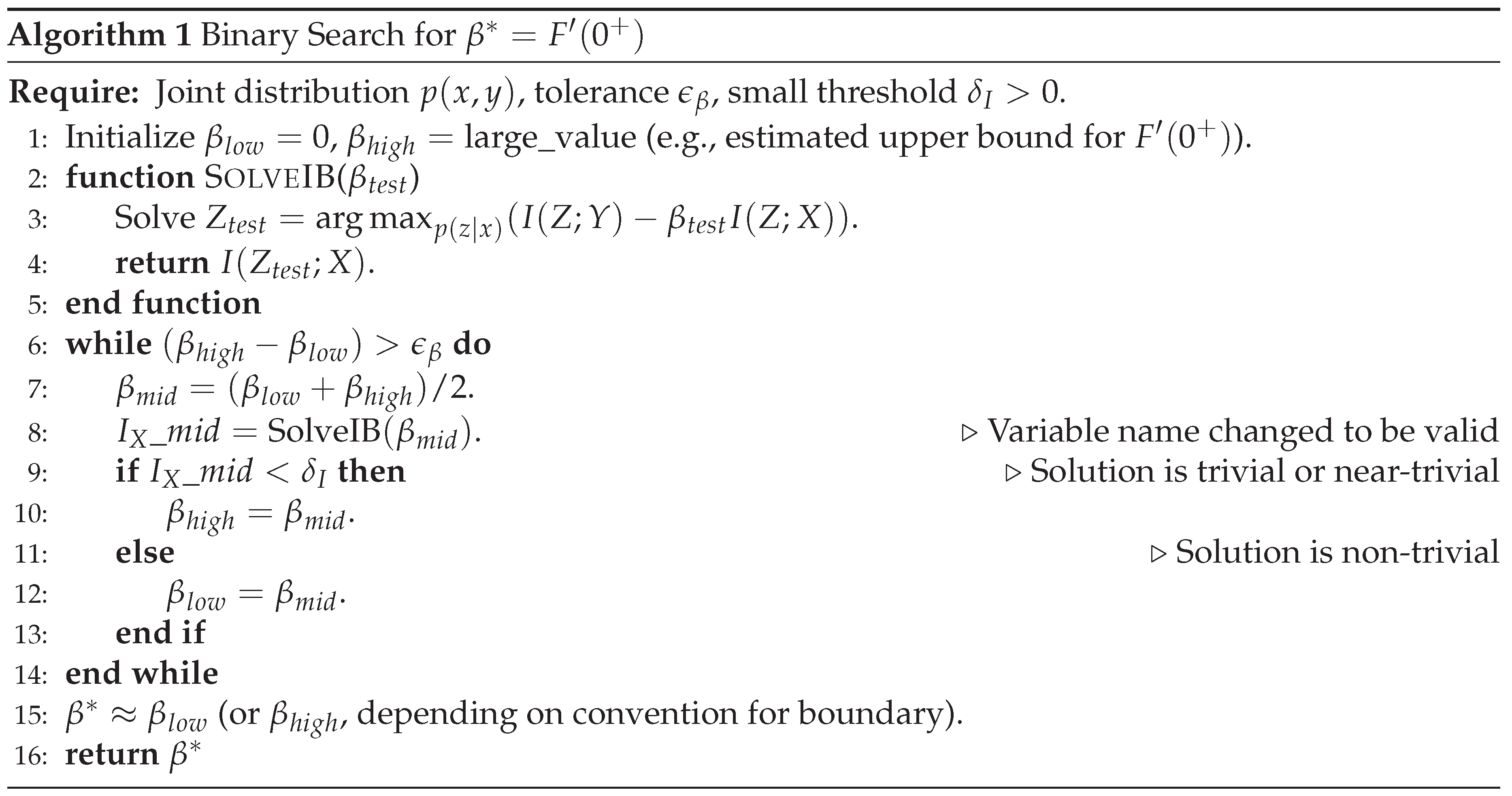
This algorithm seeks the largest $\beta$ for which the solution is non-trivial. ${\delta }_I$ is a small positive constant to numerically check for $I(Z;X)\approx 0$.

4. Discussion

4.1. ${\beta }^{*}$ in Variational IB (VIB)

In VIB [5], $\beta$ plays a similar role, but several factors can affect the observed ${\beta }^{*}$:

• Approximation Error: VIB uses bounds for $I(Z;Y)$ and $I(Z;X)$. If these bounds are not tight, or if the parametric encoder/decoder families are not expressive enough, the VIB-optimized curve may differ from the true IB curve [6]. This can shift the empirically observed ${\beta }^{*}$ for collapse.
• Collapse Phenomenon: VIB models are known to exhibit a collapse phenomenon: for too large $\beta$, the encoder $q_{\varphi }\left(z\right|x)$ learns to ignore x and $q_{\varphi }\left(z\right|x)\approx p\left(z\right)$ (the prior), making $I(Z;X)\approx 0$. This empirical collapse threshold in VIB is the analogue of the theoretical ${\beta }^{*}$.
• Practical Estimation: Practitioners often find a suitable $\beta$ by sweeping values and observing validation performance. The largest $\beta$ that maintains good performance before a sharp drop could be considered an empirical estimate of a "useful" $\beta$, which might be lower than the strict collapse threshold ${\beta }^{*}=F^{\prime }\left(0^{+}\right)$ if some minimal $I(Z;Y)$ is required.

The theory of ${\beta }^{*}$ provides a target: VIB training should ideally operate with $\beta \le {\beta }^{*}$ to avoid complete information loss.

4.2. ${\beta }^{*}$ in Neural IB (NIB)

NIB approaches, like DIB [4] or methods using MINE [10], also involve a trade-off parameter analogous to $\beta$.

• Deterministic IB (DIB): DIB optimizes $I(Z;Y)-\beta H\left(Z\right)$. Since $I(Z;X)\le H\left(Z\right)$, DIB penalizes an upper bound on $I(Z;X)$. DIB tends to find deterministic encoders where $I(Z;X)\approx H\left(Z\right)$. The critical ${\beta }_{DIB}^{*}$ for collapse in DIB will exist but may have a different numerical value than ${\beta }_{IB}^{*}$ due to the different complexity term.
• MI Estimators: Using neural MI estimators for $I(Z;X)$ can be noisy. Detecting the exact ${\beta }^{*}$ where $I(Z;X)$ (and thus $I(Z;Y)$) truly vanishes can be hard. However, the principle of a collapse threshold remains.

In all NIB variants, ${\beta }^{*}$ (appropriately defined for the specific objective) marks the boundary of useful compression.

4.3. Generalization and Robustness Considerations

The IB framework is linked to generalization in machine learning [2,11]. Compressing representations (larger $\beta$) can discard irrelevant information, potentially improving generalization by preventing overfitting. ${\beta }^{*}=F^{\prime }\left(0^{+}\right)$ represents the most extreme compression. Operating slightly below ${\beta }^{*}$ might yield representations that are highly compressed yet still informative. Choosing $\beta$ to optimize generalization often involves finding a balance, possibly at a "knee" of the IB curve, which is different from ${\beta }^{*}=F^{\prime }\left(0^{+}\right)$. However, ${\beta }^{*}$ provides a hard upper limit on useful $\beta$ values. Similar arguments apply to robustness: IB might discard fragile, non-robust features.

4.4. Multi-Target or Multi-Layer Extensions

For multiple targets $Y_1,Y_2,\dots$, or for IB applied at multiple layers of a deep network [16], the concept of $\beta$-optimization becomes more complex. One might have a vector of $\beta$ parameters or layer-specific ${\beta }_i^{*}$. The fundamental idea of a critical threshold where information is lost would likely generalize, but its characterization would be more involved.

4.5. Limitations and Assumptions

The analysis relies on certain assumptions:

• Concavity and differentiability of $F\left(r\right)$: For some distributions, $F\left(r\right)$ might have kinks or linear segments. ${\beta }^{*}$ as $F^{\prime }\left(0^{+}\right)$ still exists (as a one-sided derivative).
• Existence of optimal encoders: Assumed for theoretical IB. In practice (VIB/NIB), model capacity and optimization are critical. If models are too restricted, apparent collapse might occur earlier due to capacity limits rather than $\beta$ itself.

5. Conclusion

In this work, I presented a comprehensive theoretical study of $\beta$-optimization in the Information Bottleneck framework. I formally defined ${\beta }^{*}$ as the critical Lagrange multiplier ${\beta }^{*}=F^{\prime }\left(0^{+}\right)$, which marks the boundary where the IB solution transitions from being informative (non-trivial) to uninformative (trivial). This ${\beta }^{*}$ represents the maximal compression pressure under which a representation can still convey some information about the target.

My analysis yielded the following key takeaways:

• ${\beta }^{*}$ exists and is unique for a given X–Y distribution, identifiable as $F^{\prime }\left(0^{+}\right)$ (Theorem 2). It signifies the point beyond which further increase in the compression penalty $\beta$ leads to a complete loss of information.
• The IB trade-off curve $F\left(r\right)$ is concave (Theorem 1), ensuring a well-behaved relationship between $\beta$ (as the slope $F^{\prime }\left(r\right)$) and the optimal information measures $\left(I\right(Z;X),I(Z;Y\left)\right)$.
• At ${\beta }^{*}=F^{\prime }\left(0^{+}\right)$, the representation $Z_{{\beta }^{*}}$ is maximally compressed while potentially retaining the initial, most "efficient" bits of information about Y (Theorem 3). This is distinct from concepts like minimal sufficiency for Y (i.e., $I(Z;Y)=I(X;Y)$), which occurs at the other end of the IB curve (typically $\beta \approx 0$).
• Algorithmic approaches, such as binary search (Algorithm ), can be used to estimate ${\beta }^{*}$ in practice.
• The interpretation of ${\beta }^{*}$ extends to VIB and NIB, where analogous collapse phenomena are observed, though the exact value may be affected by approximations or alternative objective formulations.

My findings offer practical guidance by providing a principled understanding of ${\beta }^{*}$. This can help reduce reliance on ad-hoc tuning. For instance, estimating $F^{\prime }\left(0^{+}\right)$ or using informed search strategies can guide the selection of $\beta$.

Future Work: Several avenues for future research emerge:

• Developing adaptive algorithms that dynamically tune $\beta$ towards ${\beta }^{*}$ (or a desired point relative to ${\beta }^{*}$) during training.
• Investigating robust estimation of ${\beta }^{*}$ from finite samples, especially in high-dimensional settings.
• Extending the theory of ${\beta }^{*}$-optimization to more complex scenarios, such as multi-target IB, sequential IB (e.g., for time-series data or reinforcement learning), or hierarchical IB in deep networks.
• Exploring the relationship between ${\beta }^{*}=F^{\prime }\left(0^{+}\right)$ and other notions of an "optimal" $\beta$, such as one corresponding to the "knee" of the IB curve or one optimizing generalization performance on a validation set. While ${\beta }^{*}=F^{\prime }\left(0^{+}\right)$ is a mathematically precise critical point, other definitions might be more relevant for specific practical goals.

In conclusion, this work grounds $\beta$-optimization in the IB framework with a formal understanding of ${\beta }^{*}$ as the critical threshold for informativeness. I hope this theoretical analysis contributes to a more principled application of the Information Bottleneck method in designing efficient and effective representation learning systems.

References

- Tishby, N., Pereira, F.C., Bialek, W. (2000). The information bottleneck method. Proc. of 37th Allerton Conference on Communication, Control, and Computing.
- Shamir, O., Sabato, S., Tishby, N. (2010). Learning and Generalization with the Information Bottleneck. In Proc. of the 2010 IEEE Information Theory Workshop (ITW).
- Chechik, G., Globerson, A., Tishby, N., Weiss, Y. (2005). Information bottleneck for Gaussian variables. Journal of Machine Learning Research, 6:165–188.
- Strouse, D.J., Schwab, D.J. (2017). The Deterministic Information Bottleneck. Neural Computation, 29(6):1611–1630. [CrossRef]
- Alemi, A.A., Fischer, I., Dillon, J.V., Murphy, K. (2017). Deep Variational Information Bottleneck. Proc. of the International Conference on Learning Representations (ICLR).
- Kolchinsky, A., Tracey, B.D., Wolpert, D.H. (2019). Nonlinear Information Bottleneck. Entropy, 21(12):1181. [CrossRef]
- Kolchinsky, A., Tracey, B.D., Van Kuyk, S. (2019). Caveats for Information Bottleneck in deterministic scenarios. Proc. of the International Conference on Learning Representations (ICLR).
- Rodríguez Gálvez, B., Thobaben, R., Skoglund, M. (2020). The Convex Information Bottleneck Lagrangian. Entropy, 22(1):98. [CrossRef]
- Wu, T., Fischer, I., Chuang, I.L., Tegmark, M. (2019). Learnability for the Information Bottleneck. Entropy, 21(10):924. [CrossRef]
- Belghazi, M.I., Baratin, A., Rajeshwar, S., Ozair, S., Bengio, Y., Courville, A., Hjelm, D. (2018). MINE: Mutual Information Neural Estimation. Proc. of the International Conference on Machine Learning (ICML).
- Achille, A., Soatto, S. (2018). Emergence of Invariance and Disentanglement in Deep Representations. Journal of Machine Learning Research, 19(54):1–34.
- Zhao, Z., Liu, Y., Peng, X., Li, Y., Liu, T., Tao, D. (2024). Exploring Complex Trade-offs in Information Bottleneck through Multi-Objective Optimization. arXiv preprint. arXiv:2310.00789.
- Liu, Y., Zhao, Z., Peng, X., Liu, T., Tao, D. (2023). Exploring the Trade-Off in the Variational Information Bottleneck for Regression with a Single Training Run. Entropy, 25(7):1043. DOI: 10.3390/e25071043. (Corrected volume/issue for 2023, assuming typical Entropy numbering. Original was 26(12):1043 which is unlikely for 2023).
- Cover, T.M., Thomas, J.A. (2012). Elements of Information Theory. Wiley, 2nd Ed.
- Witsenhausen, H.S., Wyner, A.D. (1975). A conditional entropy bound for a pair of discrete random variables. IEEE Transactions on Information Theory, 21(5):493–501.
- Shwartz-Ziv, R., Tishby, N. (2017). Opening the Black Box of Deep Neural Networks via Information. arXiv preprint. arXiv:1703.00810.
Disclaimer/Publisher’s Note: The statements, opinions and data contained in all publications are solely those of the individual author(s) and contributor(s) and not of MDPI and/or the editor(s). MDPI and/or the editor(s) disclaim responsibility for any injury to people or property resulting from any ideas, methods, instructions or products referred to in the content. |
© 2025 by the authors. Licensee MDPI, Basel, Switzerland. This article is an open access article distributed under the terms and conditions of the Creative Commons Attribution (CC BY) license (http://creativecommons.org/licenses/by/4.0/).
Copyright: This open access article is published under a Creative Commons CC BY 4.0 license, which permit the free download, distribution, and reuse, provided that the author and preprint are cited in any reuse.