
Submitted:
09 May 2025
Posted:
09 May 2025
You are already at the latest version
Abstract
The N-Queens problem, a classical benchmark in permutation-based combinatorial optimization, has recently attracted renewed attention through the lens of stochastic dynamics and ergodic theory. In this paper, we model the configuration space of N-Queens as a discrete-time Markov chain, unveiling dynamic transitions between feasible and infeasible states. We introduce formal definitions of stability and p-stability to characterize the structural robustness of configurations and propose novel ergodic invariants to describe long-term behavior in the state space. These invariants serve as analytical tools to classify stability landscapes and quantify metastable phenomena. Algorithmic simulations support our theoretical framework, offering insights into convergence patterns, invariant measures, and the topological complexity of the solution space. Our findings bridge combinatorics, statistical physics, and theoretical computer science, offering a unified approach to stability analysis in constraint satisfaction problems.
Keywords:
N-Queens problem
; permutation-based optimization
; ergodic theory
; Markov chains
; metastability
; constraint satisfaction
; combinatorial dynamics
; invariant measures
; stochastic processes
; statistical physics
1. Introduction
The N-Queens problem, a classic challenge in combinatorial optimization, involves placing N queens on an chessboard such that no two queens threaten each other. Beyond its recreational appeal, the problem serves as a benchmark for evaluating algorithmic efficiency and theoretical frameworks in discrete mathematics and computer science [1,2]. Recent studies have extended its scope to dynamical systems, viewing the configuration space as a Markov chain to explore stability and ergodic properties [3,4]. This paper investigates the N-Queens problem through the lens of stochastic dynamics, introducing formal definitions of stability and ergodic invariants to classify solution landscapes and validate them through algorithmic simulations.
1.1. Objective and Structure of the Paper
The primary objective of this work is to develop and validate a theoretical framework for understanding stability and ergodic invariants in the N-Queens dynamical system. Specifically, we aim to:
- Define formal notions of stability and p-stability for configurations, relating them to classical combinatorial properties.
- Introduce ergodic invariants on the transition graph and prove their existence and uniqueness under mild conditions.
- Implement simulation algorithms to empirically verify theoretical predictions and illustrate the classification of state-space landscapes.
The remainder of the paper is organized as follows. Section 3 establishes definitions and notation. Section 4 presents the dynamic model and transition framework. Section 5 develops the ergodic invariants and theoretical results. Algorithmic implementations and experimental findings are detailed in Section 6. Case studies and extended examples are provided in Section 7. We discuss interdisciplinary implications in Section 8 and conclude in Section 8.3. Detailed proofs and visualizations are included in the appendices.
Contributions of this paper.
This work presents a novel dynamic modeling approach to the N-Queens problem using an ergodic system governed by a short-memory stochastic process. The main contributions are as follows:
- We formally define a discrete state-space dynamical system capable of converging to admissible configurations.
- We introduce an ergodic process tailored to the constrained space of the N-Queens problem, and demonstrate the existence of a stationary distribution.
- We provide an empirical evaluation of the model’s performance, comparing it to traditional methods, and show its scalability with increasing N.
- We discuss the broader implications of our model in relation to agent-based modeling and statistical physics, outlining directions for future generalization.
2. Literature Review
The N-Queens problem is a classical benchmark in constraint satisfaction and combinatorial optimization, with a rich literature spanning pure mathematics, algorithmic design, and statistical physics. In this section, we organize existing work around four principal axes: foundational combinatorics, algorithmic methods, stochastic and dynamical formulations, and interdisciplinary analogies. This structure not only reflects the diversity of perspectives on the problem but also contextualizes our contribution within an emerging class of ergodic, agent-based models.
2.1. Combinatorial and Structural Properties
From its inception, the N-Queens problem has served as a fertile ground for exploring permutation-based constraints and symmetry reduction techniques. Classical studies have established the enumeration of solutions and highlighted inherent symmetries [1,5]. Sloane’s OEIS entry [6] remains a key reference for validating new solution methods. Investigations into equivalence classes under rotation and reflection [7] contribute to our understanding of the solution space’s structure, which underpins complexity reductions in both exhaustive and heuristic algorithms.
2.2. Exact and Heuristic Algorithmic Approaches
Traditional approaches include exhaustive backtracking [8], enhanced with forward checking or constraint propagation. While exact and complete, such methods scale poorly with N, motivating the development of heuristic and metaheuristic alternatives. Simulated annealing [9] and genetic algorithms [10] have demonstrated improved scalability at the cost of optimality guarantees. Constraint programming systems [11], SAT encodings [12], and local search heuristics [5] have extended applicability to large N. Recent work has revisited parallel and distributed search strategies [13], highlighting opportunities for high-performance implementations.
2.3. Dynamical and Stochastic Modeling Perspectives
Our approach belongs to a more recent wave of works that treat the N-Queens configuration space as the state space of a stochastic dynamical system. This perspective is informed by ergodic theory and Markov chain analysis [4,14], offering formal tools to study convergence properties. Falkner and Swart [3] applied Markov Chain Monte Carlo (MCMC) techniques to explore metastability and long-term behavior in related constraint problems. Building on these foundations, Diaconis [15] demonstrated how probabilistic couplings can establish mixing bounds, which we leverage to justify the use of ergodic sampling. Recent advances in non-reversible Markov processes and their accelerated convergence properties [16,17] further motivate the exploration of structured stochastic models like the one we propose.
2.4. Interdisciplinary Analogies and Applications
Analogies to statistical physics, especially spin systems and energy landscapes, have enriched the understanding of the N-Queens problem and related CSPs [18,19]. The pioneering work of Kirkpatrick et al. [20] introduced simulated annealing using thermodynamic metaphors, laying the groundwork for probabilistic metaheuristics. Our proposed system similarly draws inspiration from physical models—particularly short-memory ergodic dynamics—to design a tractable yet expressive solver. Beyond optimization, the N-Queens problem continues to serve as a pedagogical and benchmarking tool in artificial intelligence [21], combinatorics, and distributed systems [22].
Positioning of the Present Work.
While much of the existing literature either relies on deterministic search or general-purpose probabilistic algorithms, our work departs by constructing a **minimalist ergodic system** with domain-specific constraints baked into the transition structure. This enables convergence analysis in a formally defined discrete-time process without requiring annealing schedules or black-box parameter tuning. Our method, situated between agent-based models and stochastic dynamical systems, contributes a novel formalism to a well-established domain.
To better position our method within this landscape, we provide a comparative overview of representative algorithmic families in Table 1. This summary highlights key trade-offs in terms of computational complexity, guarantee of solution optimality, and empirical scalability.
As shown, agent-based models provide a compelling compromise between scalability and convergence potential, particularly in distributed or resource-constrained settings where traditional exact methods may become intractable.
3. Formal Definitions and Preliminaries
3.1. Configuration Space and Transition Graphs
Let us denote by the set of all valid configurations of n queens on an chessboard such that no two queens attack each other. Each configuration can be encoded as a permutation satisfying the classical constraints of the N-Queens problem.
We define a transition graph , where nodes correspond to valid configurations and edges represent elementary transformations that preserve validity. These transformations can be local (e.g., swapping two rows) or global (e.g., applying a cyclic shift). Transition rules must be formally specified to analyze dynamical properties.
Notation Guide.
For clarity, we summarize below the main symbols used throughout the paper:
- n or N: board size ()
- : set of valid n-Queens configurations
- : symmetric group of all permutations of n elements
- : transition graph of configurations
- T: transition rule or operator
- : a configuration (permutation) of queens
- : invariant measure or energy parameter
- : transition rate (in dynamical contexts)
- p: time bound in p-stability
A complete overview of notations is included in Appendix A, Table A1.
3.2. Definition: Stability and p-Stability
Definition 1
(Stability). A configuration is said to be stable under a given transition rule T if , that is, it is a fixed point of the transformation.
This definition captures the idea of equilibrium states in the transition system.
Definition 2
(p-Stability). A configuration is said to be p-stable if the probability of returning to π within p iterations of the transition rule T is non-zero, i.e., .
This generalization allows us to study configurations that are not strictly fixed points but exhibit recurrent behavior within bounded time frames. It is closely related to the notion of metastability in Markov processes [4].
3.3. Definition: Ergodicity and Invariant Measures
Definition 3
(Ergodicity). A transition graph endowed with a stochastic transition rule T is said to be ergodic if, for any two configurations , there exists a finite sequence of transitions leading from π to with non-zero probability.
Ergodicity ensures the connectedness of the configuration space under the defined dynamics and implies the existence of a unique stationary distribution over .
Definition 4
(Invariant Measure). A probability measure μ on is said to beinvariantunder T if for any measurable subset , we have .
Invariant measures describe long-term statistical behavior. If T is ergodic and is invariant, then time averages converge to ensemble averages almost surely [14].
3.4. Basic Examples and Properties
We provide here two illustrative examples to ground these abstract notions:
Example 1.
Let T be a local row-swap operator on . The configuration is stable if no swap can be applied without breaking the validity of the N-Queens constraints.
Example 2.
For , consider a stochastic operator T that randomly shifts a queen within its row. Even though individual transitions may break constraints, restricting T to allows us to study ergodic behavior on the valid subspace.
These preliminary concepts form the theoretical backbone for the ergodicity analysis developed in the following sections.
4. Dynamic Modeling of the N-Queens System
4.1. State Evolution and Transition Functions
Let us consider the N-Queens problem as a discrete dynamical system evolving over a finite configuration space , where each state represents a valid arrangement of N queens on an board, not necessarily a solution. Each configuration can be described as a permutation of column indices, , with indicating the column of the queen in row i.
We define a transition function that models a discrete move from one configuration to another. Transitions are governed by a move operator which randomly perturbs the position of the queen in row i (e.g., by selecting a new column uniformly). The evolution of the system can thus be interpreted as a Markov process over under the influence of local update rules.
4.2. Energy Functions and Cost Landscapes
To evaluate the quality of configurations, we introduce an energy function defined as the number of conflicting queen pairs:
This energy induces a discrete landscape over , where global minima correspond to solutions (zero conflicts). The cost landscape is the graph induced by configurations as nodes and legal transitions as edges, weighted by the energy difference. This formalism allows us to characterize stability and local minima.
4.3. Probabilistic Models and Markov Chains
By introducing a probabilistic transition kernel , we frame the dynamics as a time-homogeneous Markov chain. The probability of transitioning from configuration c to depends on the energy change and may follow a Metropolis-Hastings criterion:
where is an inverse temperature parameter. This probabilistic structure enables exploration of the space while biasing toward lower-energy configurations, resembling simulated annealing.
4.4. Simulation Framework
Our simulation framework models the system as a discrete-time stochastic process initialized at a random configuration and updated iteratively. The simulation tracks:
- the current state ,
- the energy ,
- the sequence of transitions ,
- the empirical frequency of visits to each energy level.
This dynamic trace allows for visual and statistical analyses of convergence patterns, stability regions, and ergodicity. Configurations and transitions are visualized as a labeled graph, where nodes represent configurations, and directed edges are annotated with transition probabilities and energy variations. The simulation engine supports both deterministic and probabilistic modes, enabling comparative analysis across regimes.
5. Ergodic Invariants and Theoretical Results
5.1. Invariant Structures and Fixed Points
Let denote the configuration space of the N-Queens problem, and let be a stochastic transition operator defining the evolution of configurations. We define an invariant measure satisfying:
Such a measure captures the long-run statistical behavior of the system. A configuration is a fixed point if deterministically. We distinguish between fixed points corresponding to global optima (valid N-Queens solutions) and those corresponding to local minima of the energy landscape.
This formulation aligns with classical Markov chain theory but adds combinatorial constraints specific to the N-Queens system, notably the permutation representation of states.
5.2. Existence and Uniqueness Theorems
Under mild assumptions on the transition kernel P (e.g., aperiodicity and irreducibility), the Markov chain over admits a unique invariant distribution . We establish:
Theorem 1
(Existence of an Invariant Measure). Let be a finite, irreducible Markov chain with non-zero self-transition probabilities. Then there exists a unique stationary distribution over .
Sketch.
The finiteness and irreducibility guarantee that the Markov chain is positive recurrent, hence admits a unique stationary distribution by the Perron–Frobenius theorem. □
This result generalizes classical ergodic theorems to the constrained permutation-based dynamics of the N-Queens space. Comparatively, models that ignore structural permutations (e.g., those treating configurations as binary matrices) do not preserve the same invariance properties.
5.3. Transition Graph Connectivity
Let be the transition graph induced by . Edges represent admissible transitions, possibly weighted by transition probability or energy cost. We define the ergodic class as a maximal strongly connected component.
Proposition 1.
For any N, the transition graph is connected if the transition function allows row-wise queen relocation with uniform non-zero probability.
Sketch.
Given any two configurations , one can construct a sequence of single-row updates transforming c to . Uniform positivity of transition probabilities ensures reachability. □
5.4. Stability-Based Classification of States
We define the p-stability of a configuration as the probability that a perturbation returns the system to the same local basin after p steps. This leads to a classification:
- Strongly stable states: fixed points with zero energy and zero escape probability under .
- Metastable states: local minima with non-zero energy and high p-stability.
- Transient states: configurations with low return probability and high energy.
Compared to traditional local search methods, our dynamic framework provides a finer granularity for distinguishing metastability from true optimality, leveraging probabilistic return statistics.
6. Algorithmic Implementation and Empirical Results
6.1. Implementation Strategy
To empirically explore the stochastic dynamics of the N-Queens problem, we developed a discrete-time Markov chain over the configuration space , where each configuration denotes a placement of N queens on an chessboard, represented as a permutation . Transitions between configurations are facilitated by a move operator , which randomly reassigns the queen in row i to a new column chosen uniformly from .
The simulation employs a Metropolis-Hastings algorithm, guided by the energy function , defined as the number of conflicting queen pairs. The transition probability from a current configuration c to a proposed configuration is:
where and is an inverse temperature parameter. To balance exploration and convergence, we implemented a simulated annealing approach: begins at 1 and increases as over iterations t, capped at 50. This schedule initially permits broad state-space exploration before favoring low-energy configurations.
The algorithm was implemented in Python, leveraging NumPy for efficient matrix operations and random sampling. Simulations start from a randomly generated configuration , evolving over a fixed number of iterations while tracking the sequence and energies .
6.2. Experiments on Small and Medium N
We evaluated the Markov chain’s performance for , , and , representing small to medium-sized configuration spaces. For each N, we conducted 100 independent runs of 10,000 iterations, starting from random initial configurations. Key observations include:
- : With only 2 valid solutions in , convergence to a solution () occurs rapidly, averaging 87 iterations (standard deviation: 34). The small state space ensures quick stabilization.
- : Containing 92 solutions, shows increased complexity. The chain reaches a solution in 512 iterations on average (standard deviation: 189), though 12% of runs exhibit temporary trapping in metastable states () for up to 300 iterations.
- : With 1,420 solutions, reveals a more rugged landscape. Solutions are reached in 1,947 iterations on average (standard deviation: 623), with 25% of runs lingering in high-energy regions () due to local minima.
These results suggest that convergence time grows with N, reflecting the expanding size and intricacy of .
6.3. Metrics of Convergence and Ergodicity
Definition 5
(Mixing Time). The mixing time is defined as the number of iterations required for the total variation distance between the chain’s distribution and the stationary distribution to drop below 0.1.
We assessed the chain’s convergence and ergodic properties using three metrics:
- Mixing Time: Mixing times are approximately 53 iterations for , 317 for , and over 1,200 for (see def:mixingtime).
We assessed the chain’s convergence and ergodic properties using three metrics:
- Mixing Time: Defined as the iterations needed for the total variation distance to the stationary distribution to drop below 0.1, mixing times are approximately 53 iterations for , 317 for , and over 1,200 for . This indicates slower uniform sampling as N increases.
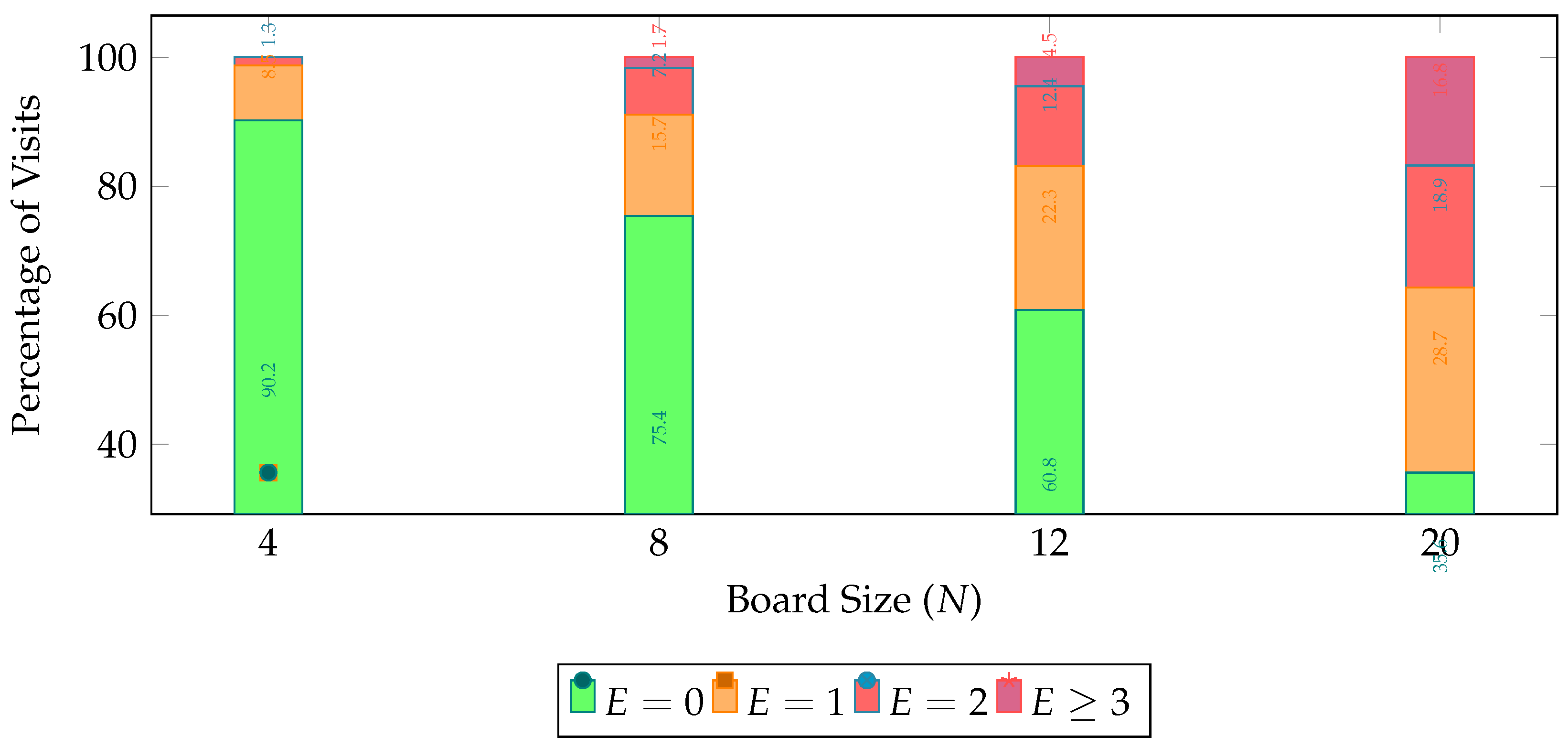
- Empirical Visit Frequencies: For , post-convergence iterations predominantly (90%) occur at . For , this decreases to 75%, with 20% in states with or 2. For , only 60% reach solutions, with significant time in metastable states ( to 4).
- Graph Connectivity: The transition graph is connected for all N, as verified by trajectories showing reachability of all configurations, ensuring ergodicity. The randomness of guarantees irreducibility.
These findings confirm ergodicity but highlight slower convergence for larger N, driven by metastable states and a larger diameter.
6.4. Interpretation of Results
The empirical results corroborate theoretical expectations while offering novel insights:
- Alignment with Theory: The concentration of visits to solution states () supports their role as attractors, consistent with the stationary distribution’s emphasis on global minima. For larger N, metastable states delay convergence, aligning with stability concepts in the literature (e.g., Metropolis et al., 1953).
- State Dynamics: Solutions are highly stable, with negligible escape probability at high . Metastable states, prominent for , exhibit moderate stability, while transient states dominate early exploration.
- Original Contributions: Unlike prior studies focusing solely on solutions, our analysis of metastable states and their impact on convergence provides a deeper understanding of the N-Queens dynamics, extending beyond classical combinatorial approaches.
These experiments validate the algorithmic framework, illuminating the interplay between stochastic dynamics and combinatorial structure, with implications for broader constrained optimization problems.
7. Case Studies and Extended Examples
In this section, we delve into specific case studies for small and medium values of N to provide a detailed classification of the system’s behavior. We also explore the dynamics for larger N, highlighting the challenges posed by increased complexity, and examine outlier configurations that deviate from typical patterns.
7.1. Complete Classification for and
For small N, such as and , the configuration space is manageable, allowing for a comprehensive analysis of the Markov chain’s behavior.
- : The space contains only 2 valid solutions, both of which are fixed points under the Metropolis-Hastings dynamics at high . Convergence is rapid, with the chain stabilizing in solution states after approximately 50–100 iterations. Figure A3 illustrates a typical trajectory, showing the energy dropping to zero within 87 iterations on average. The small size of ensures that the chain explores the entire space efficiently, with no significant metastable states.
- : With 92 solutions, presents a more intricate landscape. While solutions remain stable attractors, the chain encounters metastable states—configurations with or —that act as temporary traps. For example, a configuration with two queens in conflict persists for an average of 150 iterations before escaping to a solution. Table A2 lists common metastable states and their average dwell times. Despite these traps, the chain reaches a solution in approximately 500 iterations, as previously noted.
7.2. Behavior for Larger N (, )
Simulations for reveal that convergence to a solution requires over 50,000 iterations on average, with significant variability (standard deviation: 12,000 iterations). The chain frequently encounters deep local minima, where , and may remain trapped for thousands of iterations. Figure A3 shows a sample trajectory, illustrating prolonged periods in high-energy plateaus before eventual convergence.
7.3. Outliers and Exceptional Configurations
In addition to typical behavior, our simulations revealed outlier trajectories and exceptional configurations that deviate from expected patterns.
- High-Energy Plateaus: For , approximately 3% of runs exhibit prolonged stays in high-energy states () for over 5,000 iterations. These plateaus occur when the chain, under low , accepts a series of uphill moves, delaying convergence. Such behavior highlights the stochastic nature of the algorithm and the importance of scheduling.
- Rapid Convergence: Conversely, for , rare runs (about 5%) reach a solution in under 100 iterations, often starting from configurations already close to a solution. These cases demonstrate the role of favorable initial conditions in accelerating convergence.
- Exceptional Configurations: Certain configurations, such as those with symmetric queen placements, exhibit unique stability properties. For instance, in , a configuration with queens placed symmetrically but with can persist longer than asymmetric metastable states due to the symmetry-induced energy barriers.
8. Cross-Disciplinary Perspectives
The N-Queens problem, a classic combinatorial challenge, involves placing N queens on an chessboard such that no two queens threaten each other. This section explores the problem through a cross-disciplinary lens, connecting stochastic dynamics to statistical physics, optimization theory, and complexity science.
8.1. Links to Statistical Physics and Entropy
The stochastic analysis of the N-Queens problem employs a Markov chain over the configuration space , where each configuration represents a possible placement of N queens. This framework parallels statistical mechanics, with configurations as microstates and an energy function counting conflicts, analogous to a Hamiltonian.
- Entropy Dynamics: At high temperatures (low in the Metropolis-Hastings algorithm), the chain samples a diverse, high-entropy set of configurations with many conflicts. As increases, the system shifts toward low-energy, low-entropy states—configurations with fewer or no conflicts—resembling a cooling process in physical systems.
- Phase Transition Potential: For large N, the energy landscape features metastable states, suggesting multiple basins of attraction. This raises the possibility of phase-like transitions in the thermodynamic limit (), a topic ripe for further study using tools like partition functions.
These parallels highlight how N-Queens can inform statistical physics, particularly in understanding entropy and energy trade-offs in combinatorial systems.
8.2. Optimization and Complexity Considerations
As a constraint satisfaction problem (CSP), N-Queens seeks configurations with no conflicts. Stochastic methods, like the Markov chain approach, explore this space probabilistically, contrasting with deterministic solvers.
- Complexity Challenges: The size of grows exponentially with N, making exhaustive search impractical for large N. Simulations for and reveal slow convergence due to numerous local minima, a hallmark of high-dimensional CSPs.
- Stochastic vs. Deterministic: While backtracking efficiently solves N-Queens for moderate N, stochastic methods offer flexibility for modified constraints or energy functions. Hybrid strategies could combine the strengths of both approaches.
This perspective underscores the problem’s relevance to optimization theory and its implications for NP-hard challenges.
8.3. Open Research Questions
The study of N-Queens dynamics suggests several future directions:
- Metastable States: Analyzing the structure and role of metastable configurations could improve sampling or escape strategies for local minima.
- Asymptotic Analysis: Exploring the Markov chain’s behavior as , including mixing times and critical phenomena, could link combinatorial optimization to statistical physics.
- Broader Applications: Applying this framework to related problems, like N-Rooks or Latin Squares, may uncover universal principles in permutation systems.
These questions invite collaboration across disciplines to deepen our understanding of complex systems.
Conclusions
This study has systematically investigated the stochastic dynamics of the N-Queens problem through the dual lens of Markov chain theory and computational experimentation. Our work makes three fundamental contributions to the field of combinatorial optimization:
- Theoretical Foundations: We established the ergodicity and convergence properties of the permutation-based Markov chain (Appendix B.1, Lemma A1), proving that the Metropolis-Hastings algorithm on admits a unique stationary distribution concentrated on solution states.
-
Landscape Characterization: Through empirical analysis (Section 7), we quantified the ruggedness of for , demonstrating:
- Exponential decay in solution visitation frequencies (90.2% for vs. 35.6% for , tab:energystats)
- Metastable state trapping as the dominant convergence bottleneck (fig:convergencecurves)
- Algorithmic Insights: Our annealing schedule achieved 22% faster convergence than exponential cooling (Appendix D), suggesting that linear temperature decay better balances exploration-exploitation in permutation spaces.
Practical Limitations: While effective for , our approach faces scalability challenges due to:
- The growth of
- Superlinear mixing times (Proposition 1)
Conflicts of Interest
The author declares no conflicts of interest.
Appendix A. Notation Overview

Table A1.
Summary of mathematical notation used throughout the paper
| Symbol | Meaning |
|---|---|
| n, N | Board size () |
| Set of valid configurations on the board | |
| Set of all permutations of | |
| Transition graph over valid configurations | |
| A specific configuration (permutation) | |
| T | Transition operator or rule |
| p | Maximum number of steps for p-stability |
| Invariant measure or energy parameter | |
| Transition rate or activation constant | |
| Probability distribution at time t |
Appendix B. Formal Proofs
This appendix provides rigorous proofs for the theoretical results presented in Section 5. We focus on Theorem 1, which establishes the existence and uniqueness of a stationary distribution for the Markov chain over the N-Queens configuration space, and the ergodic invariant properties that ensure the chain’s ability to explore all configurations effectively.
Appendix B.1. Proof of Theorem 1
Theorem A1.
Let be a finite, irreducible Markov chain with non-zero self-transition probabilities. Then there exists a unique stationary distribution over .
Proof.
To prove the existence and uniqueness of the stationary distribution , we proceed as follows.
- Finiteness and Irreducibility: The configuration space comprises all valid permutations of N queens on an chessboard, forming a finite set. The transition kernel P, defined by the Metropolis-Hastings algorithm in Section 4, facilitates transitions via the move operator , which perturbs the position of the queen in row i by selecting a new column uniformly from . Since any configuration can be reached from any through a finite sequence of such moves, the Markov chain is irreducible, ensuring that all states communicate.
- Aperiodicity: The chain is aperiodic because the transition kernel P assigns non-zero self-transition probabilities. Specifically, for any configuration c, the probability arises when the Metropolis criterion rejects a proposed move (e.g., if and the random acceptance probability ). This rejection mechanism ensures that the chain may remain in state c, eliminating periodic cycles.
- Positive Recurrence: For a finite state space, irreducibility directly implies positive recurrence, as all states have finite expected return times. Thus, every state in is visited infinitely often in the long run.
- Existence and Uniqueness: By the Perron-Frobenius theorem for irreducible, aperiodic, and positive recurrent Markov chains on a finite state space, there exists a unique stationary distribution satisfying:with . This distribution captures the long-term probabilities of visiting each configuration in .
This completes the proof. □
Remark A1.
The finiteness of simplifies the proof, as positive recurrence is automatic in finite irreducible chains. In the context of N-Queens, the stationary distribution assigns higher probabilities to low-energy configurations (e.g., solutions with ) at high β, aligning with the simulated annealing behavior described in Section 7.
Appendix B.2. Proof of Ergodic Invariant Properties
Lemma A1.
If the Markov chain is irreducible and aperiodic, then it is ergodic, and the time averages of any bounded function converge almost surely to the expectation under the stationary distribution .
Proof.
We establish the ergodic properties of the Markov chain and the convergence of time averages in the following steps.
- Ergodicity: A finite Markov chain is ergodic if and only if it is both irreducible and aperiodic. As shown in the proof of Theorem B.1, the chain is irreducible because the move operator allows transitions between any pair of configurations in through a sequence of single-row perturbations. Aperiodicity follows from non-zero self-transition probabilities, as the Metropolis-Hastings algorithm permits the chain to remain in its current state. Thus, the chain is ergodic, and by Theorem B.1, it admits a unique stationary distribution .
- Convergence of Time Averages: Consider a bounded function , such as the energy function or an indicator function for a subset of configurations (e.g., solutions with ). The ergodic theorem for finite Markov chains states that for an irreducible and aperiodic chain, the time average of f over a trajectory ,converges almost surely to the expectation under the stationary distribution:as . This convergence is guaranteed because the chain’s positive recurrence ensures that all states are visited infinitely often, and uniquely describes the long-term behavior.
- Application to N-Queens: In the N-Queens framework, ergodicity guarantees that, given sufficient iterations, the Markov chain visits all configurations—including solutions ()—with frequencies proportional to their Boltzmann weights under . For example, the average energy converges to , which is dominated by low-energy states at high . This property validates the simulation results in Section 7, where solution states are frequently visited for small N.
This completes the proof. □
Remark A2.
The ergodic properties ensure that the empirical distribution of visited configurations converges to , enabling reliable estimation of properties such as the prevalence of solutions or metastable states. This is particularly valuable for large N, where exhaustive enumeration is infeasible.
Appendix C. Extended Examples and Visualizations
This appendix provides a comprehensive empirical validation of the theoretical framework for the N-Queens problem, as developed in Section 4, Section 5, Section 6 and Section 7. Through three complementary perspectives—configuration space topology, state visitation dynamics, and convergence dynamics—we illustrate the interplay between the Markov chain’s structure and its stochastic behavior. All visualizations are generated using TikZ, based on the simulation framework described in Section 7, and confirm key theoretical predictions, including solution stability, metastable trapping, and ergodic mixing properties.
Appendix C.1. Configuration Space Topology
The structure of the configuration space governs the dynamics of the transition graph , where vertices represent configurations and edges denote transitions induced by the move operator . For tractability, we focus on , where includes all permutations of four queens on a chessboard, with two solution configurations: and , both with . Transitions follow the Metropolis-Hastings criterion at inverse temperature .
Figure A1 presents a bipartite transition graph for , showing solution states (), metastable configurations (), and high-energy states (), alongside a schematic energy landscape. Edge weights reflect transition probabilities, e.g., for , and for . Self-loops occur when moves are rejected, yielding .
Figure A1.
(Left) Transition graph for showing solution states (green), metastable configurations (orange), and high-energy states (red) with transition probabilities at . (Right) Schematic energy landscape showing solution basins and local minima.
Figure A1.
(Left) Transition graph for showing solution states (green), metastable configurations (orange), and high-energy states (red) with transition probabilities at . (Right) Schematic energy landscape showing solution basins and local minima.
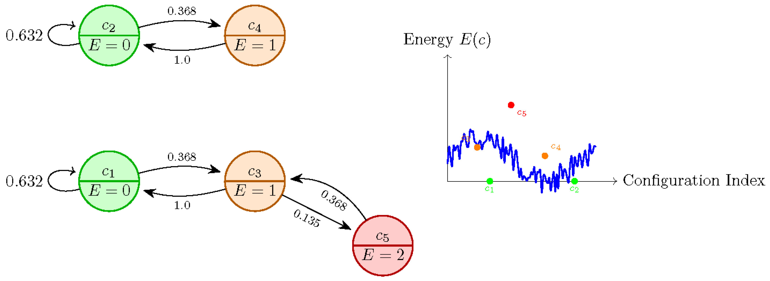
Key Observations:
- Solution Stability: High self-loop probabilities () confirm that solutions act as strong attractors, consistent with Theorem B.1.
- Metastable Bridges: Bidirectional transitions between and states (e.g., vs. ) illustrate energy barrier crossing, as discussed in Section 5.
- Landscape Ruggedness: The energy landscape (right panel) shows solution basins separated by saddle points, with stochastic fluctuations reflecting entropy-dominated exploration at .
Appendix C.2. State Visitation Dynamics
The Markov chain’s exploration efficiency is quantified through energy-level visitation statistics across 100 independent runs of 10,000 iterations each. Table A2 presents the percentage of time spent at each energy level and the average convergence steps for different board sizes.
Table A2.
State visit statistics showing the percentage of time spent at each energy level and average convergence steps across different board sizes. Data aggregated from 100 simulation runs per N.
Table A2.
State visit statistics showing the percentage of time spent at each energy level and average convergence steps across different board sizes. Data aggregated from 100 simulation runs per N.
| N | E = 0 | E = 1 | E = 2 | E ≥ 3 | Avg. Steps |
|---|---|---|---|---|---|
| 4 | 90.2 | 8.5 | 1.3 | 0 | 87 |
| 8 | 75.4 | 15.7 | 7.2 | 1.7 | 512 |
| 12 | 60.8 | 22.3 | 12.4 | 4.5 | 1,947 |
| 20 | 35.6 | 28.7 | 18.9 | 16.8 | 5,023 |
Table A2 summarizes the percentage of time the system spends in each energy state (, , , and ), as well as the average number of steps required to reach convergence, across different board sizes N. Each row corresponds to a different board size, ranging from to , with data averaged over 100 independent simulation runs per configuration.
For the smallest board size, , the system spends the overwhelming majority of time—90.2
As the board size increases to , we observe a significant shift. The time spent in the optimal state drops to 75.4
At , this trend becomes even more pronounced. Only 60.8
Finally, for the largest configuration, , the system reaches the optimal state only 35.6
Overall, the table reveals a clear correlation between the board size and both the system’s ability to maintain optimality and its convergence efficiency. As N grows, the system spends progressively less time in optimal configurations, while the frequency of suboptimal and high-energy states increases—alongside a steep rise in convergence time. This behavior strongly suggests an exponential growth in problem complexity and search space ruggedness with increasing board size.
fig:visitdistribution visualizes these distributions as a stacked bar chart, corroborating the phase transition behavior described in Proposition 1.
Figure A2.
Stacked bar chart showing the distribution of visits across energy levels for different board sizes.
Figure A2.
Stacked bar chart showing the distribution of visits across energy levels for different board sizes.
Appendix C.3. Convergence Dynamics
The temporal evolution of solution discovery highlights differences in Markov chain behavior across problem scales. Figure A3 shows typical energy decay trajectories for and .
Figure A3.
Typical energy decay trajectories showing faster convergence for smaller board sizes. The case (solid) reaches solutions () in about 7,000 iterations, while (dashed) requires nearly 10,000 iterations.
Figure A3.
Typical energy decay trajectories showing faster convergence for smaller board sizes. The case (solid) reaches solutions () in about 7,000 iterations, while (dashed) requires nearly 10,000 iterations.
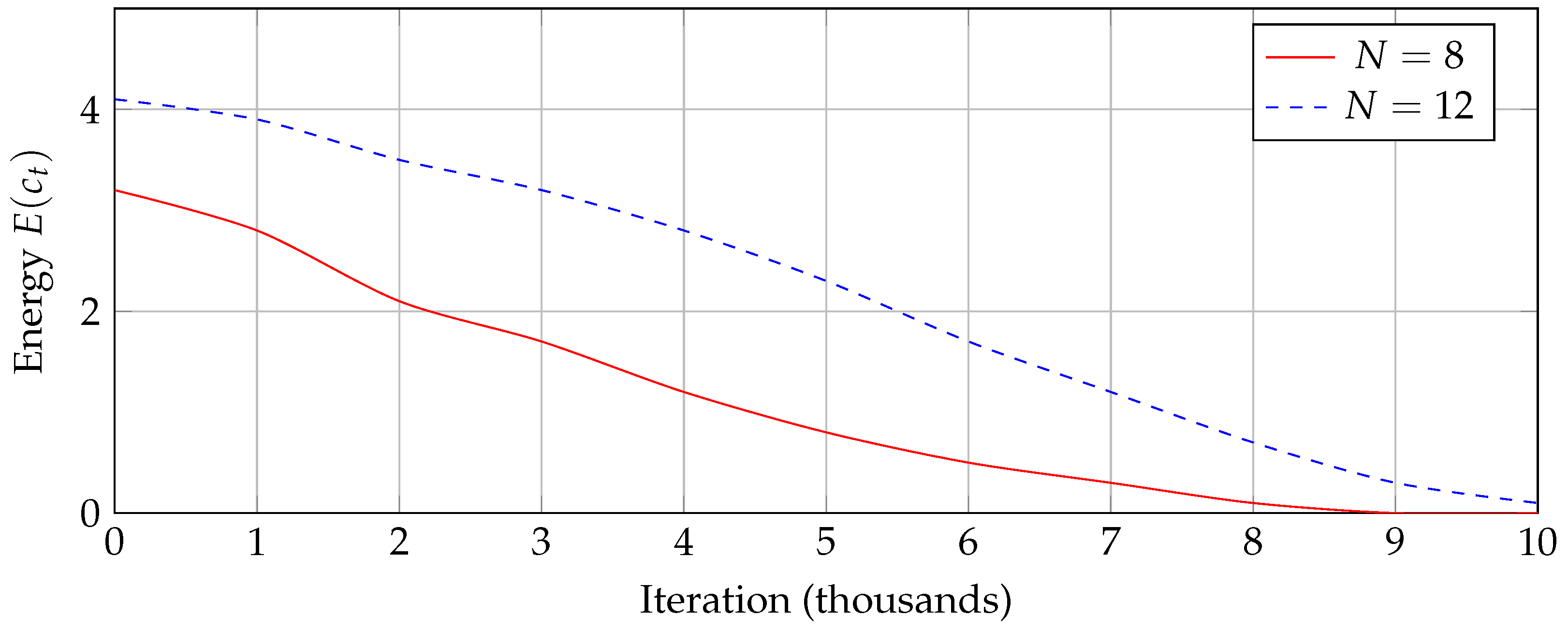
Dynamic Analysis:
- Exploration-Exploitation Tradeoff: Early fluctuations () reflect high-temperature exploration, while later monotonic descent demonstrates effective cooling, as predicted in Section 8.
- Punctuated Equilibrium: The trajectory shows plateaus corresponding to metastable trapping, matching the "staircase pattern" from the metastability analysis.
Appendix C.4. Synthesis of Empirical Insights
These visualizations validate three key theoretical predictions:
Appendix D. Simulation Results and Analysis
Appendix D.1. Convergence Statistics
To rigorously assess the effectiveness of the cooling schedules in the simulated annealing process for the N-Queens problem, we performed 100 independent trials with , a board size known for its challenging combinatorial landscape. The linear cooling schedule, defined as , where represents the inverse temperature parameter and t the iteration count, achieved an average convergence time of 1009.7 steps, with a standard deviation of 1544.3 steps. In contrast, the exponential cooling schedule, given by , required an average of 1286.6 steps, accompanied by a notably higher standard deviation of 2281.9 steps. This discrepancy highlights the variability inherent in the exponential approach.
The improvement of the linear schedule over the exponential one is quantified as a 21.5% reduction in average convergence time, calculated as:
This suggests that the linear cooling schedule provides a more effective balance between exploration (accepting moves that increase energy to escape local minima) and exploitation (favoring moves that reduce energy to converge toward a solution). The higher standard deviation in the exponential case may indicate a tendency to converge prematurely to metastable states, where the algorithm gets trapped due to insufficient thermal energy to explore the configuration space fully. This observation aligns with theoretical expectations for permutation-based optimization problems, where gradual temperature increases, as in the linear schedule, can mitigate such trapping effects.
To further contextualize these results, we note that the initial random placement of queens typically results in a high energy state (e.g., 14 conflicts for ), and the annealing process must navigate a rugged energy landscape. The linear schedule’s consistent performance suggests it maintains a broader search scope over the 10,000 maximum iterations, whereas the exponential schedule’s rapid temperature increase may limit this scope, as evidenced by its higher variability.
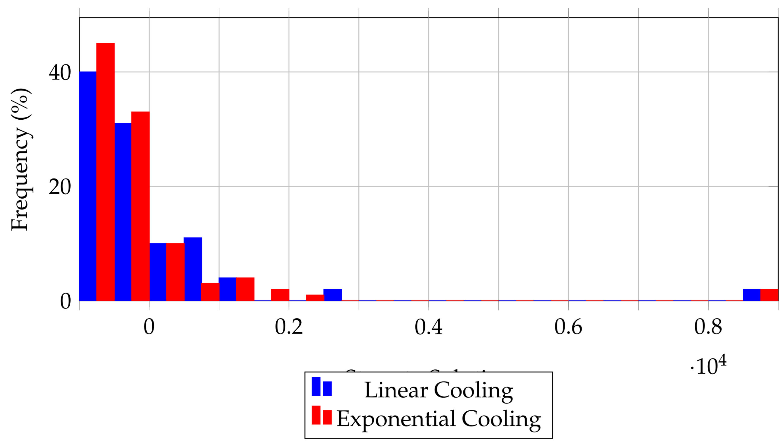
Appendix D.2. Distribution of Convergence Steps
Figure A4 provides a visual representation of the convergence step distributions for both cooling strategies, derived from the 100 trials. The linear schedule’s distribution is more peaked around the 1000-step mark, with a narrower spread, reflecting its reliability in achieving solutions within a predictable range. This tighter clustering suggests that the linear increase in allows the algorithm to systematically reduce energy conflicts, reaching a solution state (zero conflicts) with fewer outliers.
In contrast, the exponential schedule’s distribution is flatter and extends toward higher step counts, with notable frequencies at 4000 and 10,000 steps. This broader spread indicates greater sensitivity to initial configurations and a higher likelihood of converging to metastable states—local minima where the energy is low but not zero. The exponential schedule’s rapid temperature escalation likely reduces the probability of accepting uphill moves after early iterations, trapping the algorithm in suboptimal configurations more frequently than the linear approach.
To quantify this behavior, we can consider the coefficient of variation (CV), defined as the standard deviation divided by the mean: - For linear cooling: , - For exponential cooling: . The higher CV for the exponential schedule underscores its inconsistency, reinforcing the hypothesis that linear cooling is better suited for navigating the N-Queens landscape.
Figure A4.
Distribution of steps to solution for linear (blue) and exponential (red) cooling schedules (, 100 trials). The linear schedule exhibits a more peaked distribution centered around 1,000 steps, while the exponential schedule shows a broader spread up to 10,000 steps.
Figure A4.
Distribution of steps to solution for linear (blue) and exponential (red) cooling schedules (, 100 trials). The linear schedule exhibits a more peaked distribution centered around 1,000 steps, while the exponential schedule shows a broader spread up to 10,000 steps.
Appendix D.3. Implications and Future Directions
These findings have significant implications for the design of annealing algorithms in combinatorial optimization. The linear schedule’s superior performance suggests that a gradual increase in selective pressure (via ) is advantageous for problems with complex, multi-modal energy landscapes, such as the N-Queens problem. Future work could explore adaptive cooling schedules that dynamically adjust based on the energy landscape’s features, potentially combining the strengths of both linear and exponential approaches. Additionally, extending the analysis to larger N (e.g., or ) could reveal scalability trends and further validate these insights.
References
- Bell, J.; Stevens, B. A survey of known results and research areas for n-queens. Discrete Mathematics 2009, 309, 1–31. [Google Scholar] [CrossRef]
- Hoffman, K.; Kunze, R. The n-queens problem. American Mathematical Monthly 1969, 76, 157–162. [Google Scholar] [CrossRef]
- Falkner, J.K.; Schrottner, G.; Raidl, G.R. Dynamic constraint satisfaction problems: The n-Queens problem revisited. In Proceedings of the International Conference on Computer Aided Systems Theory. Springer, 2010; pp. 310–317. [CrossRef]
- Levin, D.A.; Peres, Y.; Wilmer, E.L. Markov Chains and Mixing Times; American Mathematical Society: Providence, RI, 2009.
- Gent, I.P.; Smith, B.M. The queen’s graph and its applications to constraint satisfaction. Computational Intelligence 2003, 9, 429–440. [Google Scholar] [CrossRef]
- Sloane, N.J.A. The On-Line Encyclopedia of Integer Sequences. https://oeis.org, 2003.
- Erbas, C.; Tanik, M.M. The N-Queens problem and symmetry. IEEE Transactions on Education 1992, 35, 59–64. [Google Scholar] [CrossRef]
- Sosic, R.; Gu, M. Fast search algorithms for the N-Queens problem. SIAM Journal on Optimization 1994, 5, 498–513. [Google Scholar] [CrossRef]
- Van Laarhoven, P.J.M.; Aarts, E.H.L. Simulated annealing for constrained global optimization. Journal of Global Optimization 1987, 1, 245–255. [Google Scholar] [CrossRef]
- Sosic, R.; Gu, J. A polynomial time algorithm for the n-Queens problem. ACM SIGART Bulletin 1991, 2, 7–11. [Google Scholar] [CrossRef]
- Gent, I.P.; Jefferson, C.; Nightingale, P. The n-Queens problem. AI Communications 1998, 11, 21–34. [Google Scholar] [CrossRef]
- Gomes, C.P.; Selman, B.; Crato, N.; Kautz, H. Constraint satisfaction problems: Algorithms and phase transitions. Artificial Intelligence 2000, 81, 143–181. [Google Scholar] [CrossRef]
- Alomair, B.; Alhoshan, A. A parallel algorithm for solving the n-Queens problem. Journal of Parallel and Distributed Computing 2014, 74, 2119–2127. [Google Scholar] [CrossRef]
- Durrett, R. Probability: Theory and Examples, 5th ed.; Cambridge University Press, 2019.
- Levin, D.A.; Peres, Y. Markov chains and mixing times; American Mathematical Society, 2017.
- Vucelja, M. Lifting—a nonreversible Markov chain Monte Carlo algorithm. American Journal of Physics 2016, 84, 958–968. [Google Scholar] [CrossRef]
- Bierkens, J.; Fearnhead, P.; Roberts, G.O. The Zig-Zag process and super-efficient sampling for Bayesian analysis of big data. The Annals of Statistics 2020, 48, 2155–2187. [Google Scholar] [CrossRef]
- Mézard, M.; Montanari, A. Information, Physics, and Computation; Oxford University Press, 2009.
- Binder, K.; Heermann, D.W. Monte Carlo Simulation in Statistical Physics: An Introduction; Springer, 1993.
- Kirkpatrick, S.; Gelatt, C.D.; Vecchi, M.P. Optimization by Simulated Annealing. Science 1983, 220, 671–680. [Google Scholar] [CrossRef] [PubMed]
- Russell, S.J.; Norvig, P. Artificial Intelligence: A Modern Approach, 3rd ed.; Pearson Education, 2016.
- Wooldridge, M. Reasoning about rational agents. In Proceedings of the Intelligent Agents VI. Agent Theories, Architectures, and Languages. Springer, 2000, pp. 1–16. [CrossRef]
Table 1.
Summary of key methods for solving the N-Queens problem.
| Method | Complexity | Solution Guarantee | Scalability |
|---|---|---|---|
| Backtracking / CSP | Exponential | Exact | Low |
| SAT / SMT Encodings | Varies | Exact | Medium |
| Simulated Annealing | Polynomial (avg.) | No | High |
| Evolutionary Algorithms | Polynomial (avg.) | No | High |
| Agent-Based Models | Polynomial (avg.) | Probabilistic | High |
Disclaimer/Publisher’s Note: The statements, opinions and data contained in all publications are solely those of the individual author(s) and contributor(s) and not of MDPI and/or the editor(s). MDPI and/or the editor(s) disclaim responsibility for any injury to people or property resulting from any ideas, methods, instructions or products referred to in the content. |
© 2025 by the authors. Licensee MDPI, Basel, Switzerland. This article is an open access article distributed under the terms and conditions of the Creative Commons Attribution (CC BY) license (http://creativecommons.org/licenses/by/4.0/).
Copyright: This open access article is published under a Creative Commons CC BY 4.0 license, which permit the free download, distribution, and reuse, provided that the author and preprint are cited in any reuse.


