Robust and Scalable Quantum Repeaters Using Machine Learning

Diego Fuentealba; Jackson Dahn; James Steck; Elizabeth Behrman

doi:10.20944/preprints202505.0691.v1

Submitted:

08 May 2025

Posted:

09 May 2025

You are already at the latest version

Abstract

Quantum repeaters are integral systems to quantum computing and quantum communication, as they allow the transfer of information between qubits, particularly over long distances. Because of the “no-cloning theorem,” which says that entangled quantum states cannot be directly copied, one cannot perform signal amplification in the usual way. The standard approach uses entanglement swapping, in which quantum states are teleported from one (short) segment to the next, using at each step a shared entangled pair. This is the job of the repeater. However, this requires reliable quantum memories and shared entanglement resources, which are vulnerable to noise and decoherence. Using a swap gate is also possible; however, it is difficult to manually create and implement the quantum algorithm for this circuit as the size of the system increases. Here we propose a different approach: To use machine learning to train a repeater node. To demonstrate the feasibility of this method, the system is simulated in MATLAB. Training is then done for a system of 2 qubits. It is then scaled up, with no additional training, to systems of 4, 6, and 8 qubits using transfer learning. Finally, the systems are tested in noisy conditions. The results show that scale-up is very effective and relatively easy, and the effects of noise and decoherence are reduced as the size of the system increases.

Keywords:

quantum repeater

;

machine learning

;

robust

;

scalable

;

noise

;

decoherence

;

quantum communication

Subject:

Physical Sciences - Quantum Science and Technology

Introduction and Literature Review

Large scale quantum communication networks face a unique (quantum) problem: Standard (classical) amplification of the signal is impossible because a quantum state cannot be copied [1,2]. Thus the attenuation of the signal from the scattering or absorption of the photons as they travel through optical fibers (or air) needs to be addressed in a different way. Quantum repeaters provide one solution for dealing with this. The standard approach uses entanglement swapping, in which quantum states are teleported from one (short) segment to the next, using at each step a shared entangled pair [3,4,5]. Note that this necessitates also a reliable set of quantum memories at each node, to store the entangled pairs used to perform the teleportation. Great progress has been made in all of the contributing components to this protocol: Researchers have demonstrated entanglement swapping operations, quantum memories, and even on a small scale the full quantum networks. But the field is still in flux in the sense that no one technology or physical implementation has been settled on [6,7,8] and many difficulties remain. A major issue is noise and decoherence effects. To deal with these, one can use some form of error correction, such as entanglement purification [3,9]. Substantial progress still needs to be made, and new approaches [10,11,12] need to be tried. For example, Liu et al. [10] propose returning to the old idea of vacuum beam guides in place of optical fibers, as they offer orders of magnitude lower loss; Mastriani [12] presents a simplified version of entanglement swapping that is less expensive for quantum repeaters.

In our research presented here, building on our prior quantum machine learning work, we propose a different kind of simplification: To use quantum machine learning [13] to perform all the necessary operations. In this way, we bypass the quantum memory and its attendant measurements. Scaleup is easy, as we use transfer learning to leverage knowledge of the larger from the smaller system [14,15]. This transfer learning could be called “bootstrapping”, a term we have coined in past work for this process when thinking about how a classical computer uses a small “boot sector” program to launch a much larger OS. Most important, because of the parallel and distributed nature of the trained quantum neural network architecture, the resultant operation is robust to both noise and decoherence [16], analogously to the way classical neural networks have long been successfully used to deal with incomplete or damaged data. In fact, the network becomes more robust as the system size increases [17], which is a major result of our work presented here. In general using this kind of approach to a number of problems, we have found that the tedious complexity of developing quantum algorithms by hand can be forgone, handing the task over to a machine learning system. It also frequently shortens and/or simplifies a sequence from one found by the so-called “lego” method, using gates as building blocks [18,19].

Methodology

System Description

The quantum system used in this research has the parameters K for tunneling,

ϵ

, bias and

ζ

, coupling coefficients, and the Hamiltonian is constructed from these parameters as:

H = \sum_{i = 1}^{n} K_{i} σ_{x, i} + \sum_{i = 1}^{n} ϵ_{i} σ_{z, i} + \frac{1}{2} \sum_{i \neq j}^{n} ζ_{i, j} σ_{z, i} σ_{z, j}

where

K_{i}

is the tunneling amplitude for qubit i,

ϵ_{i}

is the bias for qubit i,

ζ_{i, j}

is the coupling coefficient between the i j pair of qubits in the system, and

σ_{x}

and

σ_{z}

are the Pauli spin matrices.

The parameters K,

ϵ

, and

ζ

of the Hamiltonian are time dependent, as then so is H. The quantum system state variable is the density matrix,

ρ

, which evolves from an initial

ρ_{0}

at t=0 to a

ρ^{f}

at the final time

t_{f}

according to the Schrodinger equation

\frac{d ρ}{d t} = \frac{1}{i h} [H, ρ]

(1)

The quantum parameters are trained using machine learning to achieve a final target density matrix at the final time

ρ^{f} = T

. So, an initial

ρ_{0}

paired with a target

ρ^{f} = T

represents the required quantum state change. More details about this are given later. The time dependence of each parameter is represented as a finite Fourier series, and the Fourier coefficients are trained using an adjoint Levenberg-Marquardt machine learning method also described below.

Cost Function with Frobenius Output Measure

The quantum system evolves in time according to the Schrodinger equation, from an initial density matrix

ρ_{0}

to a final density matrix

ρ^{f}

at the final time

t_{f}

. Recall that the Hamiltonian, H, is time varying. A cost function, L, is defined as a positive definite error based on the Frobenius norm of a matrix. T is the target output density matrix for the quantum system and

ρ

at

t^{f}

is the actual quantum system output density matrix. The system dynamics are enforced as a constraint with Lagrange multiplier vectors

γ

and

λ

.

\begin{matrix} L = \sum {(T_{i j} - ρ_{i j})}^{†} (T_{i j} - ρ_{i j}) |_{t_{f}} + \int_{0}^{t_{f}} γ^{†} [\frac{d ρ}{d t} - \frac{1}{i h} [H, ρ]] λ d t \\ + \int λ^{†} {[\frac{d ρ}{d t} - \frac{1}{i h} [H, ρ]]}^{†} γ d t \end{matrix}

(2)

Taking the variation w.r.t.

γ λ

and setting it equal to zero enforces the Schrodinger equation dynamics. Integrating the first term in each integral by parts and taking the variation w.r.t.

ρ

and setting that equal to zero at any time

t < t_{f}

gives

\frac{d γ λ}{d t} = - \frac{1}{i h} [H, γ λ]

(3)

and its complex conjugate equation. Note that since

ρ

is specified at t=0, its variation at that initial time is zero, and that initial condition term vanishes. At

t_{f}

we have (and its conjugate):

γ λ_{i j} = (T_{i j} - ρ_{i j})

(4)

The Hamiltonian, H, contains parameters mentioned above which describe how H varies with time. Let w be one of these parameters. Taking the variation of L with respect to w gives a gradient of L that can be used in various gradient based adaptation methods to determine the parameter.

\frac{δ L}{δ w} = \int_{0}^{t_{f}} 2 R e [\frac{1}{i h} γ^{t} [\frac{d H}{d w}, ρ] λ]

(5)

Following mainly [20] which is based on the Levenberg-Marquardt method of nonlinear optimization presented in [21] [22] and [23] we derive a quasi-second order method for learning the quantum parameters in H. Levenberg-Marquardt outperforms gradient descent and conjugate gradient methods for medium sized problems.

Let

W

be a vector of the quantum parameters. L is a function of

W

, so we define

[\frac{\partial L}{\partial W}]

as a vector of partials of L w.r.t. each element of W and then define

\hat{L}

as a quadratic (2nd order) local approximation to L about

W_{0}

the current value of the quantum parameter vector as

\begin{matrix} \hat{L} (W) = L (W_{0}) + {[\frac{\partial L}{\partial w}]}_{W}^{T} 0 (W - W_{0}) \\ + \frac{1}{4 L (W_{0})} (W - W_{0}) {[\frac{\partial L}{\partial W}]}_{W}^{T} 0 {[\frac{\partial L}{\partial W}]}_{W} 0 {(W - W_{0})}^{T} \end{matrix}

(6)

notice that

\hat{L} (W_{0}) = L (W_{0})

(7)

and

{[\frac{\partial \hat{L}}{\partial W}]}_{W} 0 = {[\frac{\partial L}{\partial W}]}_{W} 0

(8)

and

L (W_{0}) = \sum {(T_{i j} - ρ_{i j})}^{t} (T_{i j} - ρ_{i j}) |_{t_{f}}

(9)

as the forward dynamics equation constraint being enforced means the other terms in L are zero. This means

L (W_{0})

is the squared “output” error at the final time with the current parameters

W_{0}

. Then setting the variation of L w.r.t.

W

equal to 0 gives

0 = {[\frac{\partial \hat{L}}{\partial W}]}_{W} = {[\frac{\partial L}{\partial W}]}_{W} 0 + \frac{1}{L (W_{0})} (W - W_{0}) {[\frac{\partial L}{\partial W}]}_{W}^{T} 0 {[\frac{\partial L}{\partial W}]}_{W} 0 .

(10)

Then define a Hessian by

H_{e s s} = \frac{1}{\sqrt{L (W_{0})}} {[\frac{\partial L}{\partial W}]}_{W} 0 {[\frac{\partial L}{\partial W}]}_{W}^{T} 0 \frac{1}{\sqrt{L (W_{0})}}

(11)

giving

W = W_{0} - H_{e s s}^{- 1} {[\frac{\partial L}{\partial W}]}_{W}^{T} 0

(12)

The Levenberg-Marquardt algorithm modifies this by combining this Hessian update rule with a gradient descent update rule that is weighted by a parameter

λ

that is updated dynamically during the learning process. Also, the Hessian and the gradient of L become averages over all training pairs in the training set, or in a mini-batch subset, and

L (W_{0})

becomes the average squared error over the entire set, by necessity, since it could be zero for any single training data point. For details on the LM process, including updating

λ

, see [24] .

The combined weight update rule is

W = W_{0} - η {[H_{e s s} + λ I]}^{- 1} {[\frac{\partial L}{\partial w}]}_{W}^{T} 0

(13)

where

I

is the identity matrix and

η

is a constant that controls the rate of update “learning ” of the quantum parameters. The standard LM algorithm is

W = W_{0} - η {[{\hat{H}}_{e s s} + λ I]}^{- 1} E {[\frac{\partial O}{\partial w}]}_{W}^{T} 0

(14)

If we absorb

L (W_{0})

into

η

and

λ

and define the output O in the standard LM algorithm above as the squared error L, and have its target value as zero, our update using L looks much like the standard LM formulation. Because the error at the final time

γ λ_{i j} = (T_{i j} - ρ_{i j})

(15)

is propagated backward through the quantum system dynamics in equation 3, the error is contained in the gradient calculated via equation 5. Therefore the “error” E which multiplies the gradient in the standard LM algorithm is set to a vector of ones in our LM formulation.

The motivation for the approximation

\hat{L}

is as follows. Let a function of one variable, f(x), be approximated close to x=0 by the form

\hat{f (x)} = \frac{1}{2} a {(1 + b x)}^{2}

(16)

Note this form matches the form of the first term of L above. Then choose a=2f(0) to make f(0)=

\hat{f} (0)

and choose ab=

{[\frac{\partial f}{\partial x}]}_{0}

to make

{[\frac{\partial f}{\partial x}]}_{0} = {[\frac{\partial \hat{f}}{\partial x}]}_{0}

. Then

\hat{f} (x) = f (0) + {[\frac{\partial f}{\partial x}]}_{0} x + \frac{1}{4 f (0)} x^{2} {[\frac{\partial L}{\partial x}]}_{0}^{T} {[\frac{\partial f}{\partial x}]}_{0}

(17)

For small

λ

, the update rule is similar to the Gauss-Newton algorithm, allowing larger steps when the error is decreasing rapidly. For larger

λ

, the algorithm pivots to be closer to gradient descent and makes smaller updates to the weights. This flexibility is the key to L.M.’s efficacy, changing

λ

to adapt the step size to respond to the needs of convergence: moving quickly through the parameter space where the error function is steep and slowly when near an error plateau and thereby finding small improvements. Our implementation is a modified L.M. algorithm following several suggestions in [25]. One epoch of training consists of the following: 1) Compute the Jacobian

[\frac{\partial L}{\partial W}]

and then the Hessian 11 with current weights w 2) Update the damping parameter

λ

3) Calculate a potential parameter update 4) Find if RMS error has decreased with new parameters, or if an acceptable uphill step is found 5) If neither condition in step 3 is satisfied, reject the update, increase

λ

, and return to step 2 6) For an accepted parameter change, keep the new parameters and decrease

λ

, ending the epoch. The identity matrix I that multiplies

λ

can be replaced by a scaling matrix

D^{T} D

which serves the primary purpose of combating parameter evaporation [26], which is the tendency of the algorithm to push values to infinity while somewhat lost in the parameter space. Following [25], we can choose

D^{T} D

to be a diagonal matrix with entries equal to the largest diagonal entries of

H_{e s s}

yet encountered in the algorithm, with a minimum value of

10^{- 6}

. Updates to the damping factor may be done directly or indirectly; our results here use a direct method.

System Training and Training Pairs

A list of valid quantum states and the resulting paired swap must be produced to create a set of input/target output pairs to train the network. Each input, with the exception of the charge basis inputs, results from creating a ket of random, uniformly distributed probability amplitude values via a random number generator and subsequently normalizing the ket. The output is then found by multiplying the input by the appropriate swap operation matrix. In total, 74 training pairs are generated, with 70 being generated via random number generation and the remaining 4 training pairs are the charge basis.

The input/target output for each training pair can then be represented in their density matrix forms

T = ρ_{f} = | Ψ_{f} 〉 〈 Ψ_{f} |

and

ρ_{o} = | Ψ_{o} 〉 〈 Ψ_{o} |

where

Ψ_{0}

and

Ψ_{f}

are the kets of the initial “input” and target final “output” . The system Hamiltonian parameters are then trained by presenting it with an initial “input”state from the training set, the system is evolved to the final time according to the Schrodinger equation,

i ℏ \frac{\partial ρ}{\partial t} = [H, ρ]

, the co-state

γ λ

is calculated backward in time according to equation 3 and the associated element of the gradient vector is calculated according to 5. Averaging over all training pairs, the Hessian is then calculated using 11 and the parameters updated with 13. After completion of the training of the 2-qubit system, the system is then scaled up to 4-, 6-, and 8-qubits through transfer learning [14,15]. This was done by copying the tunneling, K, and bias,

ϵ

from the original 2 qubits respectively to the added 2 qubits. The coupling,

ζ

between the first 2 qubits is copied respectively to the coupling between the added 2 qubits.. There is no coupling between the old 2 and the added 2 qubits. The results of the scale-up are obtained by testing on 70 randomly generated states and

2^{n}

charge basis corresponding to system size.

Noise Simulation

Once the system is trained, the task turns to proving the systems’ resilience to noise and decoherence. There is a distinction between noise and decoherence as it is applied to this work. Pure noise is the addition of random magnitudes to the system, while decoherence is the addition of random phases to the system; the combination of these two we called “complex noise” [17]. All three of these were used to test the system. To add noise to the system, a noise matrix of small random values that is: Hermitian, positive semi-definite, and has a trace of 1 (the required properties of a valid density matrix) is produced at each time step for each training pair. This noise matrix is then added to the input state’s density matrix and normalized to produce a valid density matrix containing the desired type of noise. The trained system is then tested on specific swap tasks, that is, swap qubit A with qubit B and qubit C with qubit D, etc., depending on the size of the system. The inputs to which the noise is added for the 2-qubit system is identical to the inputs of training set. For the 4-, 6-, and 8-qubit systems, the inputs to which the noise is added is the same as the ones used to test the system after scale-up.

In the results section below we report RMS error for the training and testing datasets as well as a measure of the average amount of noise introduced for the testing results. These are calculated as follows.

RMS error for the entire testing dataset is calculated by

R M S = \sqrt{\frac{\sum_{i p a i r} {(\frac{| | T - ρ_{f} {| |}_{F R}}{N s i z e^{2}})}^{2}}{N p a i r s}}

(18)

The noise level reported below is an average over the elements of the noise matrix, all the timesteps, and all the training pairs calculated by

A v e r a g e N o i s e = \frac{\sum_{i p a i r} \sqrt{\frac{\sum_{i t i m e} {(\frac{| | ρ_{n o i s e} {| |}_{F R}}{N s i z e^{2}})}^{2}}{n t i m e s t e p s}}}{N p a i r s}

(19)

For both equations above,

{| | A | |}_{F R}

is the Frobenius norm of the matrix A.

The system is tested with varying levels of average noise and the results are presented in the following section.

Results

To first establish a baseline for training effectiveness, a two qubits system was trained on the dataset described above to sufficiently low error, and those parameters were then transferred [14,15] to the four-, six-, and eight-qubit cases with no additional training following the procedure described above. The baseline results are summarized in Table 1 for a

testing

set consisting of the charge basis states and 70 randomly generated quantum states for each system size. A jump is seen in the RMS error when scaling up from 2 to 4 qubits, but stabilizes from 4 to 6 and 6 to 8 qubits.

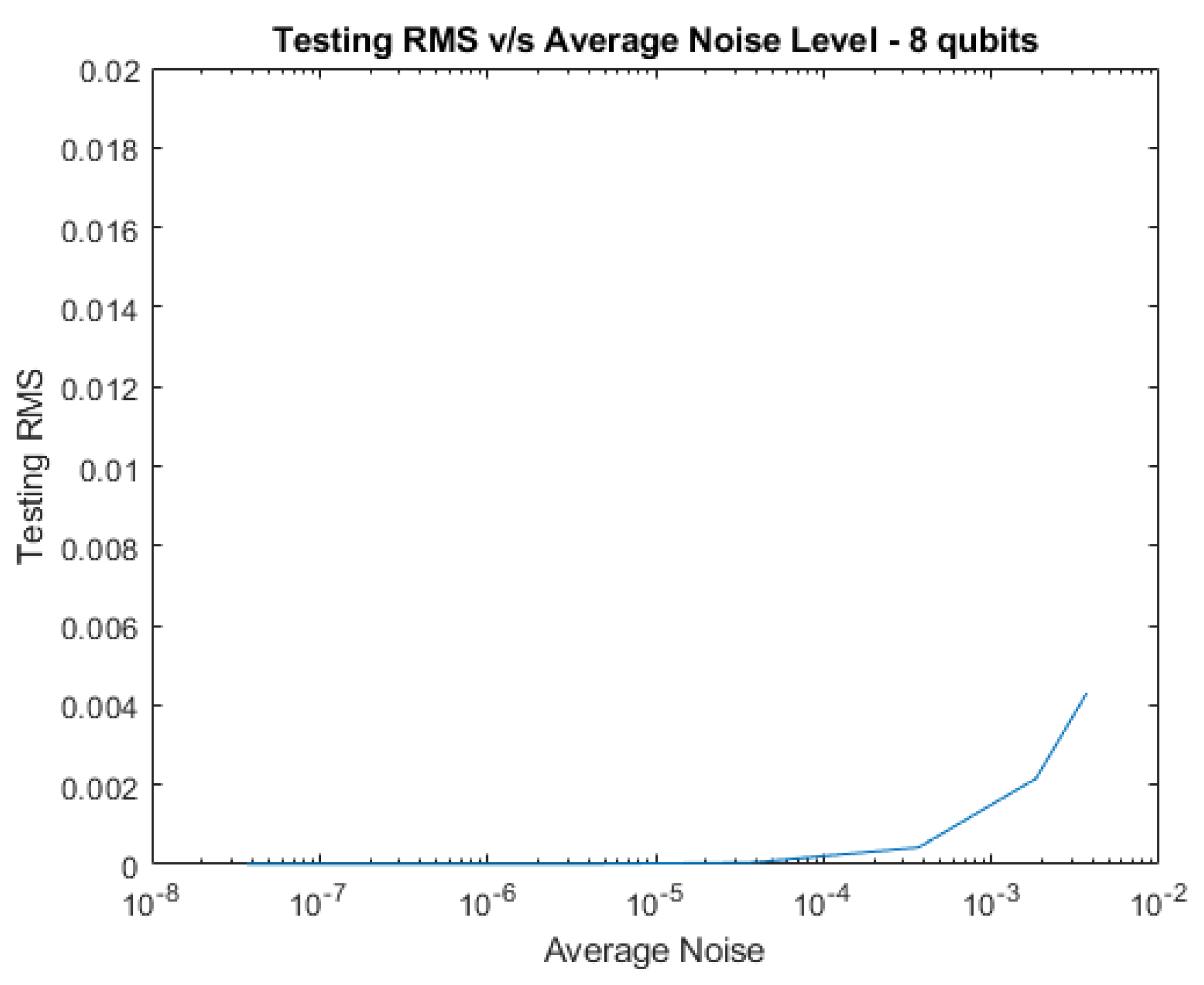
Next, noise was added to the system to test the network’s resiliency. Tests were conducted with pure noise and decoherence separately, as well as together, all at various levels and the average noise levels are reported in the tables below. RNP is a parameter that we use to generate the level of random noise numbers. The testing RMS is reported for each noise type at each RNP level. We find that the network’s noise tolerance improves as the system’s size increases, as demonstrated by the figures. Therefore, larger systems have the potential to be more noise tolerant without the need for additional training.

Table 2. Error Induced by Noise for 2 qubits

RNP	Pure Noise RMS	Decoherence RMS	Complex Noise RMS
1e-6	$1.97 \times 10^{- 5}$	$4.91 \times 10^{- 5}$	$9.44 \times 10^{- 5}$
1e-5	$2.01 \times 10^{- 4}$	$4.94 \times 10^{- 4}$	$9.44 \times 10^{- 4}$
1e-4	0.0019	0.0047	0.0085

Table 3. Error Induced by Noise for 4 qubits

RNP	Pure Noise RMS	Decoherence RMS	Complex Noise RMS
1e-6	$1.42 \times 10^{- 5}$	$2.28 \times 10^{- 5}$	$8.30 \times 10^{- 5}$
1e-5	$1.07 \times 10^{- 4}$	$1.98 \times 10^{- 4}$	$6.66 \times 10^{- 4}$
1e-4	$8.30 \times 10^{- 4}$	0.0012	0.0021

Table 4. Error Induced by Noise for 6 qubits

RNP	Pure Noise RMS	Decoherence RMS	Complex Noise RMS
1e-6	$1.03 \times 10^{- 5}$	$1.94 \times 10^{- 5}$	$9.73 \times 10^{- 5}$
1e-5	$7.24 \times 10^{- 5}$	$1.06 \times 10^{- 4}$	$1.74 \times 10^{- 4}$
1e-4	$1.72 \times 10^{- 4}$	$1.75 \times 10^{- 4}$	$1.99 \times 10^{- 4}$

Table 5. Error Induced by Noise for 8 qubits

RNP	Pure Noise RMS	Decoherence RMS	Complex Noise RMS
1e-6	$6.56 \times 10^{- 6}$	$9.26 \times 10^{- 6}$	$1.36 \times 10^{- 5}$
1e-5	$1.34 \times 10^{- 5}$	$1.36 \times 10^{- 5}$	$1.43 \times 10^{- 5}$
1e-4	$2.45 \times 10^{- 5}$	$1.39 \times 10^{- 5}$	$4.53 \times 10^{- 5}$

Plots of testing RMS vs increasing amounts of average

complex

noise level are shown below for 2, 4, 6, and 8 qubits.

Figure 1. RMS vs Average Noise Level for 2 qubits with Complex Noise.

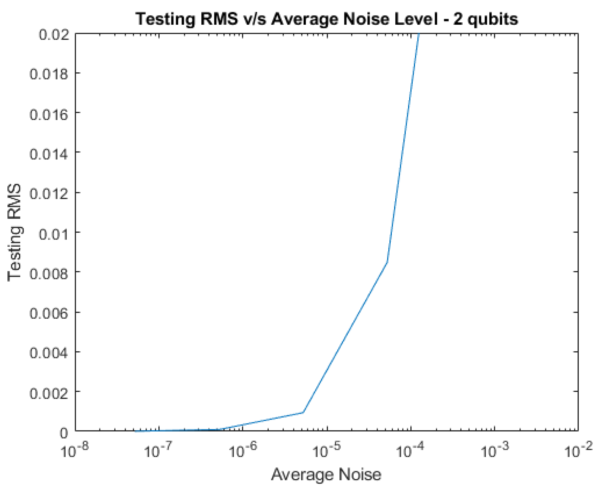
Figure 2. RMS vs Average Noise Level for 4 qubits with Complex Noise.

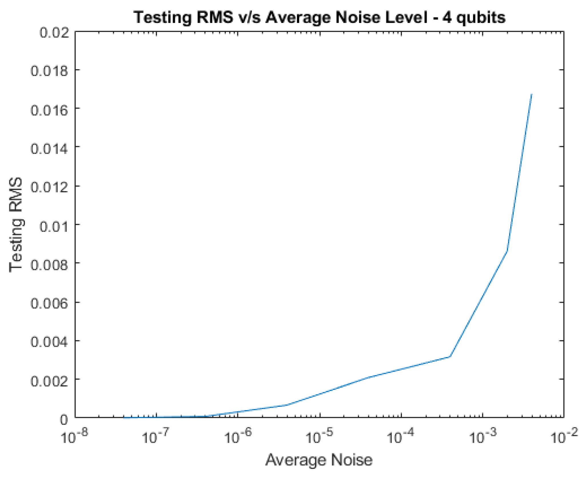
Figure 3. RMS vs Average Noise Level for 6 qubits with Complex Noise.

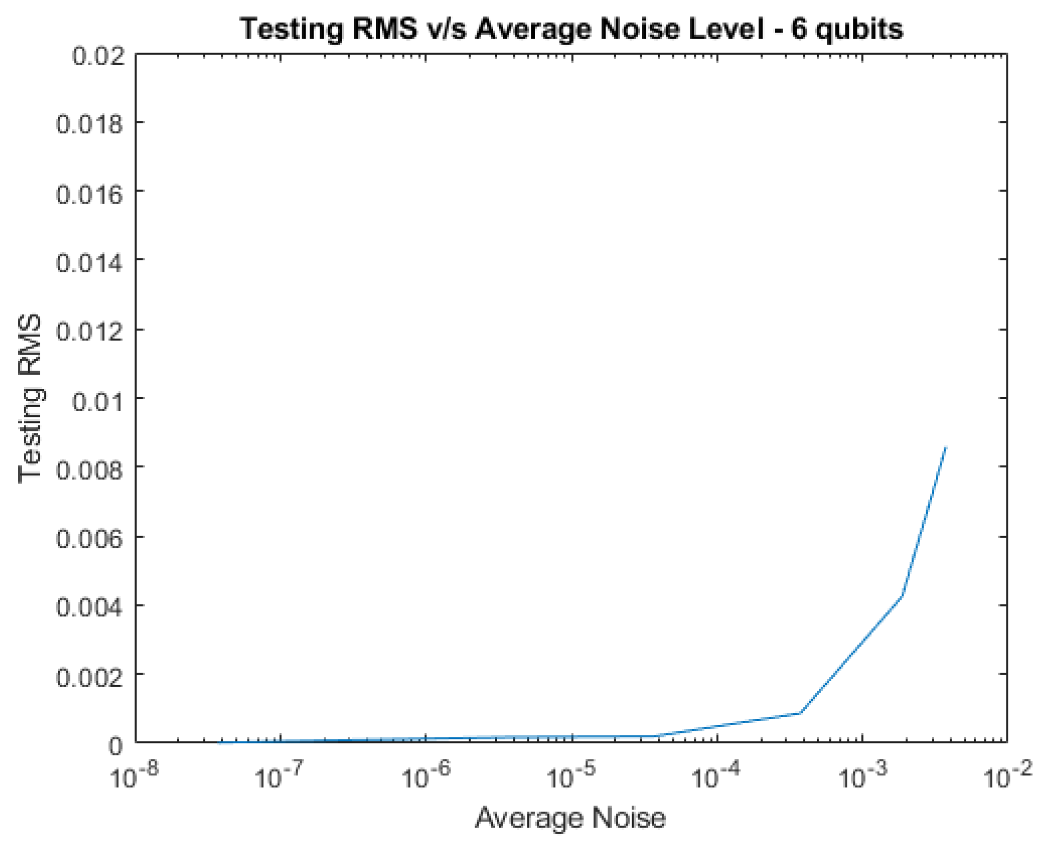
Figure 4. RMS vs Average Noise Level for 8 qubits with Complex Noise.

Conclusions and Future Research

Machine learning can be enormously helpful in both quantum computing and quantum communication for several reasons: 1) it bypasses the difficult tasks of both algorithm construction and of breaking down a desired unitary into a sequence of gates; 2) scale-up is relatively easy; and 3) the multiple inter-connectivity of the architecture leads to robustness to both noise and decoherence. In the present study we see both of those advantages: We obtain low-error swap results in the presence of noise and decoherence, and the tolerance to that noise increases as the system size increases.

Other kinds or types of noise tolerance could also be explored, for example, different spectra or models of noise. Cheng et al. showed that noise can be modeled by using matrix product density operators, which can produce effective noise models while reducing the computational power required for simulation on classical computers [27]. Noise might be added during training in addition or instead of after training. And in the future it will be interesting to see what kinds of improvements could be made were the training to be done online, on an actual quantum hardware system: We might expect to see robustness to actual physical noise and decoherence, as the network would learn to take into account the physical flaws, crosstalk, or environment actually present.

Author Contributions

Conceptualization and methodology, J.S. and E.B.; software, J.S., D.F., and J.D.; simulations and validations, J.D. and D.F.; original draft preparation, J.D. and D.F.; writing, review, and editing, D.F., J.D., J.S., and E.B. All authors have read and agreed to the published version of the manuscript.

Data Availability Statement

Requests for Matlab code, further data and information can be made via email to the authors.

Acknowledgments

We thank the entire research group for valuable discussions: Nathan Thompson, William Ingle, Anusha Krishna Murthy, Nam Nguyen.

References

Dieks, D. Communication by EPR devices. Physics Letters A 1982, 92, 271–272. [Google Scholar] [CrossRef]
Wootters, W.K.; Zurek, W.H. A single quantum cannot be cloned. Nature 1982, 299, 802–803. [Google Scholar] [CrossRef]
Briegel, H.J.; Dür, W.; Cirac, J.I.; Zoller, P. Quantum repeaters for communication, 1998, [arXiv:quant-ph/quant-ph/9803056].
Pan, J.W.; Bouwmeester, D.; Weinfurter, H.; Zeilinger, A. Experimental entanglement swapping: entangling photons that never interacted. Physical review letters 1998, 80, 3891. [Google Scholar] [CrossRef]
Shi, Y.; Patil, A.; Guha, S. Measurement-Based Entanglement Distillation and Constant-Rate Quantum Repeaters over Arbitrary Distances. 2025; arXiv:2502.11174 2025. [Google Scholar]
Zhang, Y.L.; Jie, Q.X.; Li, M.; Wu, S.H.; Wang, Z.B.; Zou, X.B.; Zhang, P.F.; Li, G.; Zhang, T.; Guo, G.C.; et al. Proposal of quantum repeater architecture based on Rydberg atom quantum processors. 2024; arXiv:2410.12523 2024. [Google Scholar]
Zajac, J.M.; Huber-Loyola, T.; Hofling, S. Quantum dots for quantum repeaters, 2025. arXiv:quant-ph/2503.13775].
Cussenot, P.; Grivet, B.; Lanyon, B.P.; Northup, T.E.; de Riedmatten, H.; Sørensen, A.S.; Sangouard, N. Uniting Quantum Processing Nodes of Cavity-coupled Ions with Rare-earth Quantum Repeaters Using Single-photon Pulse Shaping Based on Atomic Frequency Comb. 2025; arXiv:2501.18704 2025. [Google Scholar]
Chelluri, S.S.; Sharma, S.; Schmidt, F.; Kusminskiy, S.V.; van Loock, P. Bosonic quantum error correction with microwave cavities for quantum repeaters. 2025; arXiv:2503.21569 2025. [Google Scholar]
Gan, Y.; Azar, M.; Chandra, N.K.; Jin, X.; Cheng, J.; Seshadreesan, K.P.; Liu, J. Quantum repeaters enhanced by vacuum beam guides. 2025; arXiv:2504.13397 2025. [Google Scholar]
Mor-Ruiz, M.F.; Miguel-Ramiro, J.; Wallnöfer, J.; Coopmans, T.; Dür, W. Merging-based quantum repeater. 2025; arXiv:2502.04450 2025. [Google Scholar]
Mastriani, M. Simplified entanglement swapping protocol for the quantum Internet. Scientific Reports 2023, 13. [Google Scholar] [CrossRef]
Behrman, E.C.; Steck, J.E.; Kumar, P.; Walsh, K.A. Quantum algorithm design using dynamic learning. Quantum Information and Computation, vol. 8, No. 1 and 2, pp. 12-29 (2008).
Behrman, E.; Steck, J. Multiqubit entanglement of a general input state. Quantum Information and Computation 13, 36-53, 2013. [Google Scholar]
Thompson, N.; Nguyen, N.; Behrman, E.; Steck, J. Experimental pairwise entanglement estimation for an N-qubit system: A machine learning approach for programming quantum hardware. Quantum Information Processing 19, 1-18, 2020. [Google Scholar]
Behrman, E.; Nguyen, N.; Steck, J.; McCann, M. Quantum neural computation of entanglement is robust to noise and decoherence. In Quantum Inspired Computational Intelligence; Bhattacharyya, S., Maulik, U., Dutta, P., Eds.; Morgan Kaufmann: Boston, 2017; pp. 3–32. [Google Scholar] [CrossRef]
Nguyen, N.H.; Behrman, E.C.; Steck, J.E. Quantum Learning with Noise and Decoherence: A Robust Quantum Neural Network. Quantum Machine Intelligence 2(1), 1-15, 2020. [Google Scholar]
Nola, J.; Sanchez, U.; Murthy, A.K.; Behrman, E.; Steck, J. Training microwave pulses using machine learning. Academia Quantum, 2025 (to appear). [Google Scholar]
Rethinam, M.; Javali, A.; Hart, A.; Behrman, E.; Steck, J. A genetic algorithm for finding pulse sequences for nmr quantum computing. Paritantra – Journal of Systems Science and Engineering 20, 32-42, 2011. [Google Scholar]
Roweis, S. Levenberg-Marquardt Optimization. https://people.duke.edu/ hpgavin/SystemID/References/lm-Roweis.pdf.
Levenberg, K. A Method for the Solution of Certain Non-Linear Problems in Least Squares. Quarterly of Applied Mathematics 2 1944, 164–168. [Google Scholar] [CrossRef]
Marquardt, D. An Algorithm for Least-Squares Estimation of Nonlinear Parameters. Journal of the Society for Industrial and Applied Mathematics, 1963; 431–441. [Google Scholar]
More, J.J. The Levenberg-Marquardt algorithm: Implementation and theory 1978. pp. 431–441.
Steck, J.E.; Thompson, N.L.; Behrman, E.C. Programming Quantum Hardware via Levenberg-Marquardt Machine Learning. In Intelligent Quantum Information Processing; CRC Press, 2024.
Transtrum, M.K.; Sethna, J.P. Improvements to the Levenberg Marquardt algorithm for nonlinear least- squares minimization. 2012; arXiv:1201.5885 2012. [Google Scholar]
M. K. Transtrum, B.B.M.; Sethna, J.P. Geometry of nonlinear least squares with applications to sloppy models and optimization. Physical Review E 2011. [Google Scholar]
Cheng, S.; Cao, C.; Zhang, C.; Liu, Y.; Hou, S.Y.; Xu, P.; Zeng, B. Simulating noisy quantum circuits with matrix product density operators. Physical review research 2021, 3, 023005. [Google Scholar] [CrossRef]

Table 1. Noiseless RMS Values

$n_{q u b i t s}$	Trained RMS
2	$5.38 \times 10^{- 8}$
4	$9.02 \times 10^{- 6}$
6	$9.62 \times 10^{- 7}$
8	$7.32 \times 10^{- 8}$

Disclaimer/Publisher’s Note: The statements, opinions and data contained in all publications are solely those of the individual author(s) and contributor(s) and not of MDPI and/or the editor(s). MDPI and/or the editor(s) disclaim responsibility for any injury to people or property resulting from any ideas, methods, instructions or products referred to in the content.

© 2025 by the authors. Licensee MDPI, Basel, Switzerland. This article is an open access article distributed under the terms and conditions of the Creative Commons Attribution (CC BY) license (http://creativecommons.org/licenses/by/4.0/).

Copyright: This open access article is published under a Creative Commons CC BY 4.0 license, which permit the free download, distribution, and reuse, provided that the author and preprint are cited in any reuse.

Robust and Scalable Quantum Repeaters Using Machine Learning

Abstract

Keywords:

Subject:

Introduction and Literature Review

Methodology

System Description

Cost Function with Frobenius Output Measure

System Training and Training Pairs

Noise Simulation

Results

Conclusions and Future Research

Author Contributions

Data Availability Statement

Acknowledgments

References

MDPI Initiatives

Important Links

Subscribe