
Submitted:
08 May 2025
Posted:
09 May 2025
You are already at the latest version
Abstract
This paper continues a series of papers devoted to unsolved problems in the theory of stability and optimal control for
stochastic systems. A delay differential equation with stochastic perturbations of the white noise and Poisson’s jumps types
is considered. In contrast to the known stability condition, in which it is assumed that stochastic perturbations fade on the
infinity quickly enough, a new situation is studied, in which stochastic perturbations can fade on the infinity either slowly or
not fade at all. Some unsolved problem in this connection is proposed to readers attention. Besides some unsolved problems
of stabilization for one stochastic delay differential equation and one stochastic difference equation are also proposed.
Keywords:
the Wiener process
; Poisson’s measure
; general method of Lyapunov functionals construction
; asymptotic mean square stability
; stability in probability
; numerical simulation
1. Introduction
The unsolved problems proposed here continue a series of unsolved problems in stability and optimal control theory for stochastic differential and stochastic difference equations, that have been presented during the recent years at some international conferences and papers (see [1,2,3,4,5,6,7,8,9,10]). All these problems still need to be solved.
Let be a complete probability space, be a nondecreasing family of sub--algebras of , i.e., for , be the expectation with respect to the measure , be the space of -adapted stochastic processes , , .
Following Gikhman and Skorokhod [11,12], let us consider the stochastic delay differential equation
where , are -matrices, , are mutually independent standard Wiener processes, which are also independent of the Poisson measure ,
1.1. Auxiliary Definitions and Statements
Let be a solution of the Equation (1) in the time moment t, , , be a trajectory of the Equation (1) solution until the time moment t. Consider a functional that can be presented in the form , , and for put
Let D be a set of functionals , for which the function defined in (2) has a continuous derivative with respect to t and two continuous derivatives with respect to x. Let ′ be the sign of transpose, and be respectively the first and the second derivatives of the function with respect to x. For the functionals from D the generator L of the Equation (1) has the form [11,12,13]
Definition 1.
- -
- mean square stable if for each there exists a such that , , provided that ;
- -
- asymptotically mean square stable if it is mean square stable and for each initial function the solution of the Equation (1) satisfies the condition .
Theorem 1.
Some particular cases of the Equation (1) are considered in [14,15], where it is proven that if the stochastic perturbations fade on the infinity quickly enough then the asymptotically stable zero solution of the corresponding deterministic system remains asymptotically mean square stable regardless of the level of these stochastic perturbations.
In particular, in [15] the asymptotic mean square stability of the zero solution of the Equation (1) with is proven by virtue of the general method of Lyapunov functionals construction [13,16] and the method of Linear Matrix Inequalities (LMIs) [17,18,19]. By that it is supposed that for some positive definite matrix P the following conditions hold
and the Lyapunov functional is constructed in the form , where
Remark 1.
Note that in order for the constructed Lyapunov functional (5) to satisfy the conditions of Theorem 1 the integrability condition (4) of the function must be satisfied. This condition means that stochastic perturbations fade on the infinity quickly enough. Below another situation is studied. It is supposed that stochastic perturbations can fade on the infinity either slowly or not fade at all. By that some unsolved problem is also proposed.
2. About One Problem of Stability
2.1. Equation Without Delays
Consider at first the Equation (1) without delays, i.e., by the condition
Let L be the generator of the Equation (1), (6). Then via (3) for the function we have
where
Let be the norm of the matrix , i.e.,
Assume that the symmetric matrix is a negative definite matrix, i.e.,
and, besides, suppose that
Put also
Remark 2.
Theorem 2.
Proof.
Using the generator (7) and the definitions (8), (9) for and , we have
From this and Dynkin’s formula [11]
for the function it follows that
or
Integrating this inequality and using (11), we obtain
From this and it follows that and , i.e., the zero solution of the Equation (1), (6) is asymptotically mean square stable. The proof is completed. □
Remark 3.
Note that the condition (4) of integrability of the function is not a necessary condition for asymptotic mean square stability of the zero solution of the stochastic differential Equation (1). For instance, for a simple scalar equation of the type of (1) with constant coefficients
where and is the constant, i.e.,
the condition (12) holds, but the zero solution of the Equation (13) is asymptotically mean square stable if .
3. About the Problem of Stabilization by Noise
Note that the problem of stabilization has a long history, in particular, very popular problem of stabilization of the inverted pendulum is considered in a lot of works: for example, the well known work of Kapitsa [20] and many others [21,22,23,24,25,26,27,28,29,30,31,32]. Below the problem of stabilization by noise is discussed.
Consider the scalar linear Ito’s stochastic differential equation [11]
where a, b and are constants and is the standard Wiener process.
Definition 2.
and there exists such that the solution of the Equation (14) satisfies the condition
for any initial function , such that .
3.1. Equation Without Delay
Consider now the Equation (14) by the condition , i.e., without delay:
Khasminskii shows [33] that unstable by the conditions and the zero solution of the Equation (15) becomes stable by the presence of a big enough level of noise. More exactly, by the condition
so-called "stabilization by noise" occurs and the zero solution of the Equation (15) becomes stable in probability.
3.2. Purely Stochastic Equation
From the condition (16) it follows, in particular, that the zero solution of the "purely stochastic" differential equation
is stable in probability for arbitrary . Moreover, the larger , the faster the trajectories of the solution of the Equation (17) converge to zero.
Note that the solution of the Equation (17) has the form [11]
In Figure 1 one can see 4 trajectories of the solution (18) of the Equation (17) for and different values of :
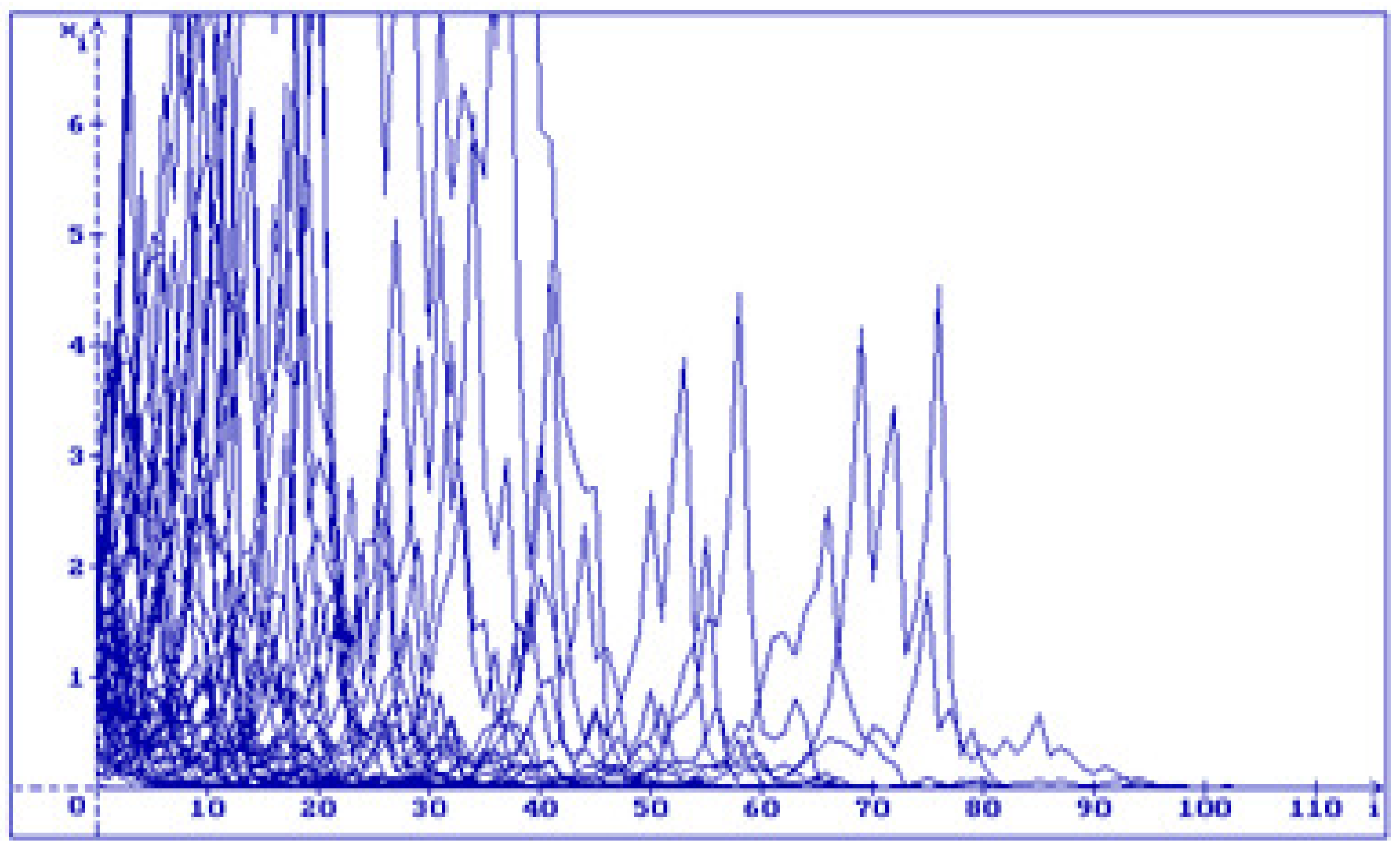
In Figure 2 one can see 50 trajectories of the solution (18) of the Equation (17) for and different values of :
A similar situation is demonstrated by 50 trajectories with negative : in Figure 3 for
and in Figure 4 for
Remark 4.
From Figs.1-4 one can see that if increases then the trajectories of the solution (18) converge to the zero faster.
Remark 5.
3.3. Stochastic Difference Equation
Consider now the scalar linear stochastic difference equation
where and are constants and , , is a sequence of mutually independent random values with the conditions
It is known that by the condition
the zero solution of the Equation (19) is asymptotic mean square stable [16].
Let us consider an analogue of the condition (16) for the linear stochastic difference Equation (19) by the condition . For this aim let us represent the difference analogue of the Equation (15) in the form (19).
Put , , , , . Then the difference analogue of the Equation (15) takes the form
Note that
satisfies the conditions (20). Using (23) rewrite the Equation (22) as follows:
i.e., in the form (19) with the coefficients
From (24) we have
and via (16) we obtain
i.e., the condition
In Figure 5 50 trajectories of the Equation (19) are shown for , and different initial conditions:
By that the condition (25) holds, all trajectories converge to the zero.
So, we obtain the following
Hypothesis 1.
Unsolved problem. Can the above reasoning be considered as a proof of the Hypothesis 1 or not? And why?
4. Conclusions
Some unsolved problems in the field of stability of differential and difference equations under stochastic perturbations are proposed to attention of potential readers. There is a hope that the solution of these problems will contribute to the emergence of new ideas and the further development and improvement of the theory of stability of stochastic systems.
Supplementary Materials
The following supporting information can be downloaded at the website of this paper posted on Preprints.org
Funding
This research received no external funding.
Data Availability Statement
No new data were created or analyzed in this study. Data sharing is not applicable to this article.
Conflicts of Interest
The author declares no conflicts of interest.
References
- Shaikhet, L. About some unsolved problems of stability theory for stochastic hereditary systems. Leverhulme International Network: Numerical and analytical solution of stochastic delay differential equations. University of Chester, UK. Abstracts, 2010, 6-7.
- Shaikhet, L. Unsolved stability problem for stochastic differential equation with varying delay. Leverhulme International Network: Numerical and analytical solution of stochastic delay differential equations. University of Chester, UK. Abstracts, 2011, 21.
- Shaikhet, L. About an unsolved stability problem for a stochastic difference equation with continuous time, Journal of Difference Equations and Applications, 2011, 17(3), 441-444. [CrossRef]
- Shaikhet, L. Two unsolved problems in the stability theory of stochastic differential equations with delay. Applied Mathematics Letters, 25(3), 636-637. [CrossRef]
- Shaikhet, L. About an unsolved optimal control problem for stochastic partial differential equation. XVI International Conference "Dynamical System Modeling and Stability Investigations" (DSMSI-2013), Kiev, 2013, 344.
- Shaikhet, L. Some Unsolved Problems: Problem 1, Problem 2. In the book: Lyapunov functionals and stability of stochastic functional differential equations. Springer Science & Business Media, 2013, 51-52.
- Shaikhet, L. Some unsolved problems in stability and optimal control theory of stochastic systems. Special Issue "Models of Delay Differential Equations-II", MDPI Mathematics, 2022, 10(3), 474, 1-10. [CrossRef]
- Shaikhet, L. About an unsolved problem of stabilization by noise for difference equations. Mathematics, 2024; 12, 110. [Google Scholar] [CrossRef]
- Shaikhet, L. Unsolved problem about stability of stochastic difference equations with continuous time and distributed delay. Modern Stochastics: Theory and Applications, 11(4), 395-402. Available online. [CrossRef]
- Shaikhet, L. About one unsolved problem in asymptotic p-stability of stochastic systems with delay. AIMS Mathematics, Special Issue: "Problems of Stability and Optimal Control for Stochastic Systems", 2024; 9, 32571–32577. [Google Scholar] [CrossRef]
- Gikhman, I.I. , Skorokhod, A.V. Stochastic Differential Equations; Springer: Berlin/Heidelberg, Germany, 1972. [Google Scholar]
- Gikhman, I.I.; Skorokhod, A.V. The Theory of Stochastic Processes, v.III; Springer: Berlin/Heidelberg, Germany, 1979. [Google Scholar]
- Shaikhet, L. Lyapunov Functionals and Stability of Stochastic Functional Differential Equations; Springer Science & Business Media: Berlin/Heidelberg, Germany, 2013. [Google Scholar]
- Shaikhet, L. About stability of delay differential equations with square integrable level of stochastic perturbations. Applied Mathematics Letters, 2019; 90, 30–35. [Google Scholar] [CrossRef]
- Shaikhet, L. Stability of delay differential equations with fading stochastic perturbations of the type of white noise and Poisson’s jumps. Discrete and Continuous Dynamical Systems Series B, 2020; 25, 3651–3657. [Google Scholar] [CrossRef]
- Shaikhet, L. Lyapunov Functionals and Stability of Stochastic Difference Equations; Springer Science & Business Media: Berlin/Heidelberg, Germany, 2011; Available online: https://link.springer.com/book/10.1007/978-0-85729-685-6 (accessed on 28 December 2024).
- Gu, K. Discretized LMI set in the stability problem of linear time-delay systems. International Journal of Control, 1997; 68, 923–934. [Google Scholar] [CrossRef]
- Fridman, E.; Shaikhet, L. Stabilization by using artificial delays: an LMI approach. Automatica, 1016; 81, 429–437. [Google Scholar] [CrossRef]
- Fridman, E.; Shaikhet, L. Simple LMIs for stability of stochastic systems with delay term given by Stieltjes integral or with stabilizing delay. Systems & Control Letters, 2019; 124, 83–91, https://www.sciencedirect.com/science/article/abs/pii/S016769111830224X. [Google Scholar]
- Kapitza, P.L. Dynamical stability of a pendulum when its point of suspension vibrates, and pendulum with a vibrating suspension. In Collected Papers of P.L. Kapitza; ter Haar, D., Ed.; Pergamon Press: London, UK, 1965; Volume 2, pp. 714–737. [Google Scholar]
- Mitchell, R. Stability of the inverted pendulum subjected to almost periodic and stochastic base motion — an application of the method of averaging. International Journal of Nonlinear Mechanics, 1972; 7, 101–123. [Google Scholar] [CrossRef]
- Levi, M. Stability of the inverted pendulum — a topological explanation. SIAM Review, 1988; 30, 639–644. [Google Scholar]
- Blackburn, J.A.; Smith, H.J.T.; Gronbech-Jensen, N. Stability and Hopf bifurcations in an inverted pendulum. American Journal of Physics, 1992; 60, 903–908. [Google Scholar] [CrossRef]
- Levi, M.; Weckesser, W. Stabilization of the inverted linearized pendulum by high frequency vibrations. SIAM Review, 1995; 37, 219–223. [Google Scholar]
- Lozano, R.; Fantoni, I.; Block, D.J. Stabilization of the inverted pendulum around its homoclinic orbit. System Control Letters. 2000, 40, 197–204. [Google Scholar] [CrossRef]
- Borne, P.; Kolmanovskii, V.; Shaikhet, L. Stabilization of inverted pendulum by control with delay. Dynamic Systems and Applications, 2000; 9, 501–514. [Google Scholar]
- Imkeller, P.; Lederer, C. Some formulas for Lyapunov exponents and rotation numbers in two dimensions and the stability of the harmonic oscillator and the inverted pendulum. Dynamical Systems, 2001; 16, 29–61. [Google Scholar] [CrossRef]
- Mata, G.J.; Pestana, E. Effective Hamiltonian and dynamic stability of the inverted pendulum. European Journal of Physics, 2004; 25, 717–721. [Google Scholar] [CrossRef]
- Sharp, R.; Tsai, Y.-H.; Engquist, B. Multiple time scale numerical methods for the inverted pendulum problem. In Multiscale Methods in Science and Engineering; Lecture Notes Computing Science and Engineering; Springer: Berlin, Germany, 2005; Volume 44, pp. 241–261. [Google Scholar] [CrossRef]
- Ovseyevich, A.I. The stability of an inverted pendulum when there are rapid random oscillations of the suspension point. Journal of Applied Mathematics and Mechanics, 2006; 70, 762–768. [Google Scholar] [CrossRef]
- Sanz-Serna, J.M. Stabilizing with a hammer. Stochastic and Dynamics, 2008; 8, 47–57. [Google Scholar]
- Shaikhet, L. About Stabilization of the Controlled Inverted Pendulum under Stochastic Perturbations of the Type of Poisson’s Jumps. MDPI, Axioms, Special Issue: “Advances in Mathematical Optimal Control and Applications”, 2025, 14(1), 29, 1-14. [CrossRef]
- Khasminskii, R.Z. Stochastic Stability of Differential Equations; Springer: Berlin/Heidelberg, Germany, 2012; (in Russian, Moscow, Nauka, 1969). [Google Scholar]
Figure 1.
4 trajectories of the solution of the Equation (17) with and 1) , 2) , 3) , 4)
Figure 1.
4 trajectories of the solution of the Equation (17) with and 1) , 2) , 3) , 4)
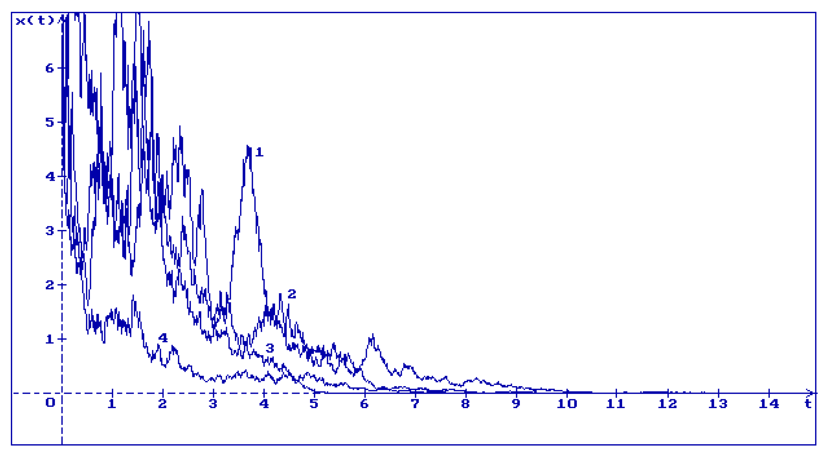
Figure 2.
50 trajectories of the solution of the Equation (17) with and 1) , 2) , ..., 49) , 50)
Figure 2.
50 trajectories of the solution of the Equation (17) with and 1) , 2) , ..., 49) , 50)
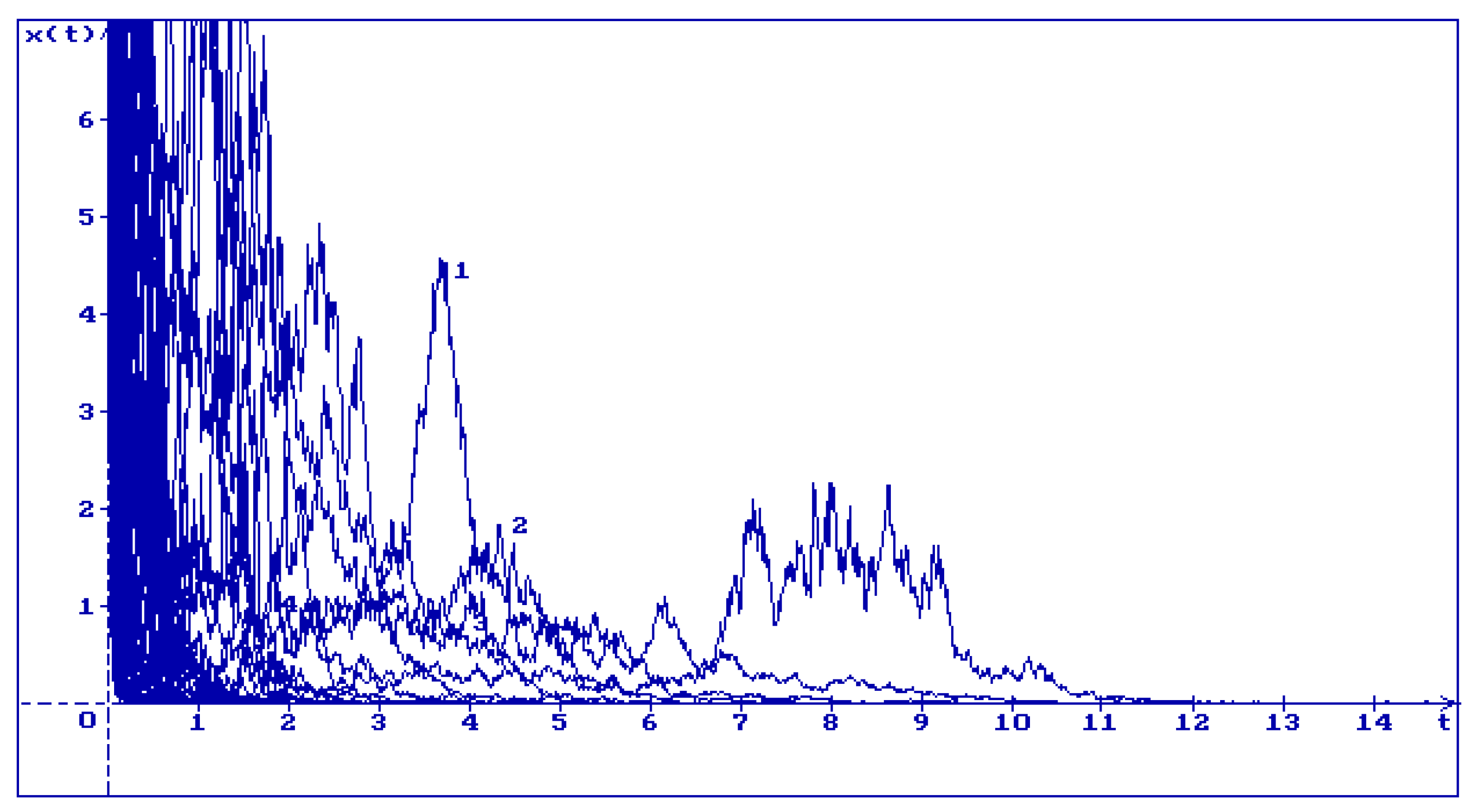
Figure 3.
4 trajectories of the solution of the Equation (17) with and 1) , 2) , 3) , 4)
Figure 3.
4 trajectories of the solution of the Equation (17) with and 1) , 2) , 3) , 4)
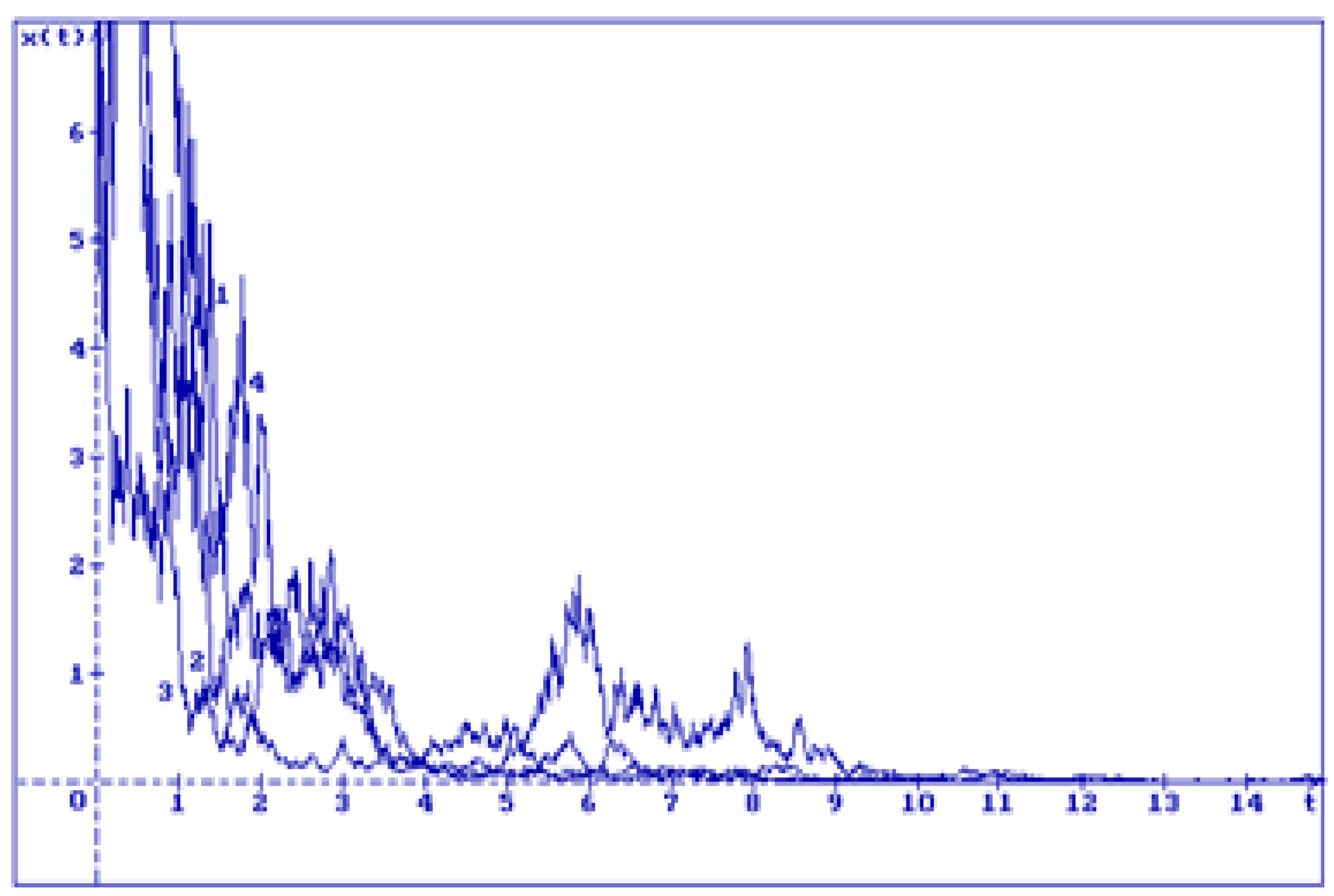
Figure 4.
46 trajectories of the solution of the Equation (17) with and 5) , 6) , ... 49) , 50)
Figure 4.
46 trajectories of the solution of the Equation (17) with and 5) , 6) , ... 49) , 50)
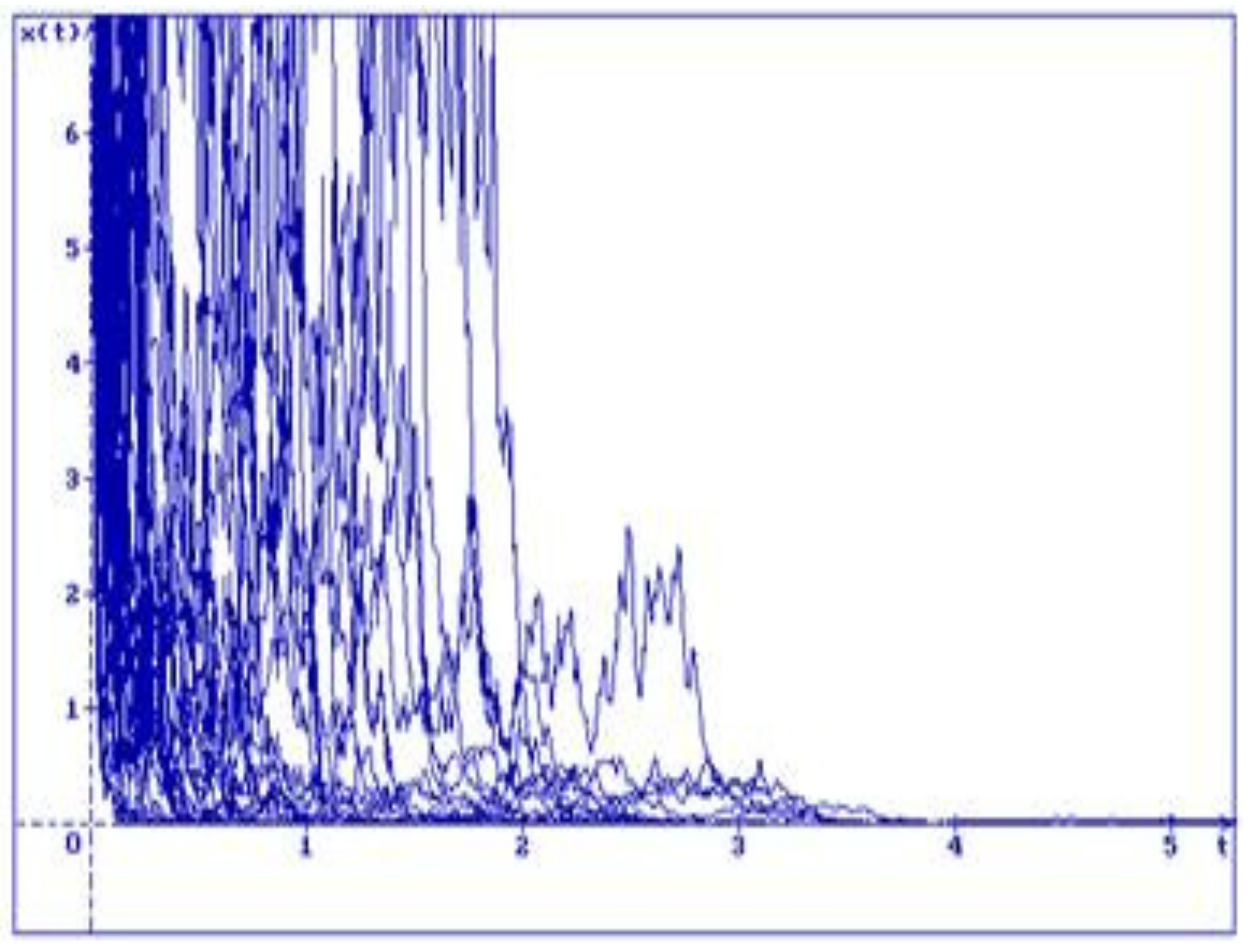
Figure 5.
50 trajectories of the solution of the Equation (19) with , and different initial conditions: 1) , 2) , ... , 49) , 50) .
Figure 5.
50 trajectories of the solution of the Equation (19) with , and different initial conditions: 1) , 2) , ... , 49) , 50) .
Disclaimer/Publisher’s Note: The statements, opinions and data contained in all publications are solely those of the individual author(s) and contributor(s) and not of MDPI and/or the editor(s). MDPI and/or the editor(s) disclaim responsibility for any injury to people or property resulting from any ideas, methods, instructions or products referred to in the content. |
© 2025 by the authors. Licensee MDPI, Basel, Switzerland. This article is an open access article distributed under the terms and conditions of the Creative Commons Attribution (CC BY) license (http://creativecommons.org/licenses/by/4.0/).
Copyright: This open access article is published under a Creative Commons CC BY 4.0 license, which permit the free download, distribution, and reuse, provided that the author and preprint are cited in any reuse.


