
Submitted:
22 June 2025
Posted:
24 June 2025
You are already at the latest version
Abstract
A system of two nonlinear difference equations under stochastic perturbations is considered. Nonlinearity of the exponential type in each equation of the system under consideration depends on all variables of the system. The stability in probability of a positive equilibrium of the system is studied via the general method of Lyapunov functionals construction and the method of linear matrix inequalities (LMIs). The obtained results are illustrated via examples and figures with the equilibrium and numerical simulation of the solution of the considered system of stochastic difference equations. The proposed research method can be applied to nonlinear systems of higher dimension and with other types of high-order nonlinearity, both for stochastic difference equations and for stochastic differential equations with delay.
Keywords:
nonlinear difference equations
; positive equilibrium
; stochastic perturbations
; asymptotic mean square stability
; stability in probability
; linear matrix inequality (LMI)
; numerical simulations
; MATLAB
MSC: 39A30; 39A50
1. Introduction
Systems of both difference and differential equations with different forms of exponential nonlinearities are very popular in research and various applications (see, for instance, [1,2,3,4,5,6,7,8,9,10,11,12] and references therein), in particular, the model of Nicholson’s blowflies [1] or Mosquito population equation [8].
Here, similarly to [10], the stability of the positive equilibrium of a system with exponential nonlinearity is investigated under stochastic perturbations via the general method of Lyapunov functionals construction [11,13,14,15] and the method of linear matrix inequalities (LMIs) [16,17,18,19,20,21,22,23,24]. However, unlike, for instance, [3,10], where the exponential nonlinearity in each equation depends on only one variable, here each equation exponentially depends on all variables of the system under consideration. The obtained results are illustrated via examples and figures with the equilibrium and numerical simulation of the solution of the considered system of difference equations. Numerical analysis of the considered LMIs is carried out using MATLAB.
Consider the system of two nonlinear difference equations
with positive parameters, , and positive initial conditions , , .
1.1. Equilibrium
It is clear that the equilibrium of the system (1) is defined by the system of two algebraic equations
It is clear that the function given by (4) is defined and positive if , where and is a unique root of the equation
which follows from (3) by .
Calculating the derivative in (4)
it is easy to see that is strictly decreasing function. Moreover, and .
Calculating the derivative of the function , defined implicitly by (6), we have
i.e., . It means that is strictly decreasing function for . Moreover, and is a unique root of the equation
which follows from (5) by . It is easy to see that the root of this equation satisfies the condition .
It is clear that two strictly decreasing functions and have (see Figure 1 and Figure 2) one common point, which is a solution of the system (2) and is the unique equilibrium of the system (1).
Remark 1.
The equilibrium of the system (1) satisfies the conditions
Example 1.
Consider the system (1) with
Then the solution of the system (2) is , from (9) and (7), (8) it follows that , , , . In Figure 1 and Figure 2 the graphs of the functions (green), (red) and the equilibrium are shown.
In Figure 1 also the asymptotes and of the functions and respectively are shown.
2. Stochastic Perturbations and the System Transformation
Let be a basic probability space, , , be a nondecreasing family of sub--algebras of , i.e., for , be the mathematical expectation with respect to the measure , and , , be two mutually independent sequences with -adapted mutually independent random values such that [11]
Let us assume that the system (1) is exposed to stochastic perturbations that are directly proportional to the deviation of the system state from the equilibrium . Then the system (1) takes the form
Remark 2.
Note that the such type of stochastic perturbations was firstly proposed in [25] for a system of Ito’s stochastic delay differential equations and was later used in many other works for both differential and difference equations (see, for instance, [11,15] and references therein). With this type of stochastic perturbations, the equilibrium of the original deterministic system remains also a solution of the stochastically perturbed system.
Presenting the solution of the system (11) in the form , we get
Similarly, for the second equation (12) we get
As a result we obtain the nonlinear system with the zero solution:
Remark 3.
3. Stability
3.1. Some Necessary Definitions and Statements
Let ′ be the transposition sign. Put now
Definition 2.([11]). The zero solution of the system (14) is called mean square stable if for each there exists a such that , , for any initial function such that ; asymptotically mean square stable if it is mean square stable and for each initial function such that the solution of the system (14) satisfies the condition .
Let be the conditional expectation with respect to the -algebra , , , and .
Theorem 2.([11]). Let for the system (14) there exists a nonnegative functional satisfying the conditions
where , . Then the zero solution of the system (14) is asymptotically mean square stable.
Remark 4.
Note that the system (13) has an order of nonlinearity higher than one. It is known [11] that in this case sufficient conditions for asymptotic mean square stability of the zero solution of the linear system (14) are also sufficient conditions for stability in probability of the zero solution of the nonlinear system (13).
3.2. Stability conditions
Theorem 3.
Let there exist positive definite -matrices P and R such that the following linear matrix inequality (LMI)
Proof.
Following the general method of Lyapunov functionals construction [11,13,14,15], consider the functional in the form , where , , is defined in (16) and the additional functional will be chosen below. For the functional via (15) we have
Using the additional functional , , with , for the functional from (21) we obtain
From (22) and the LMI (19) for some we have , i.e., the constructed functional satisfies the conditions of Theorem 2. Therefore, the zero solution of the linear equation (15) is asymptotically mean square stable. Via Remarks 4 and 3 it means that the equilibrium of the system (11) is stable in probability. The proof is completed. □
Remark 5.
4. Conclusions
Stability of a system of nonlinear difference equations under stochastic perturbations is investigated. The nonli-nearity of exponential form in each equation depends on all variables of the system under consideration. The conditions of stability in probability for positive equilibrium of the considered system, obtained via the general method of Lyapunov functionals construction, are formulated in terms of linear matrix inequalities (LMIs) and are illustrated by numerical examples and figures. The method of stability investigation, used in the paper, can be applied to many other types of systems with high-order nonlinearity, for both difference and differential equations in various applications.
Funding
This research received no external funding.
Data Availability Statement
No data was used for the research described in the article.
Conflicts of Interest
No potential conflict of interest was reported by the author(s).
References
- Q.X. Feng and J.R. Yan, Global attractivity and oscillation in a kind of Nicholson’s blowflies, Journal of Biomathematics, 17(1) (2002), pp. 21-26.
- A.Q. Khan, Global Dynamics of a Nonsymmetric System of Difference Equations, Mathematical Problems in Engineering, 14 (2022), Article ID 4435613. [CrossRef]
- G. Papaschinopoulos, M.A. Radin and C.J. Schinas, On the system of two difference equations of exponential form: xn+1=a+bxn-1e-yn, yn+1=c+dyn-1e-xn, Mathematical and Computer Modelling, 54(11) (2011), pp. 2969-2977.
- G. Papaschinopoulos, M.A. Radin and C.J. Schinas, Study of the asymptotic behavior of the solutions of three systems of difference equations of exponential form, Applied Mathematics and Computation, 218(9) (2012), pp. 5310-5318.
- G. Papaschinopoulos, N. Fotiades and C.J. Schinas, On a system of difference equations including negative exponential terms, Journal of Differential Equations and Applications, 20(5-6) (2014), pp. 717-732.
- G. Papaschinopoulos, G. Ellina and K.B. Papadopoulos, Asymptotic behavior of the positive solutions of an exponential type system of difference equations, Applied Mathematics and Computation, 245 (2014), pp. 181-190. [CrossRef]
- L. Shaikhet, Stability of equilibrium states for a stochastically perturbed exponential type system of difference equations, Journal of Computational and Applied Mathematics, 290 (2015), pp. 92-103. [CrossRef]
- L. Shaikhet, Stability of equilibrium states for a stochastically perturbed Mosquito population equation, Dynamics of Continuous, Discrete and Impulsive Systems. Series B: Applications & Algorithms, 21(2) (2014), pp. 185-196.
- L. Shaikhet, Stability of the exponential type system of stochastic difference equations, Special Issue "Nonlinear Stochastic Dynamics and Control and Its Applications", MDPI, Mathematics, 11(18) (2023), 3975, 20p.https://www.mdpi.com/2227-7390/11/18/3975.
- L. Shaikhet, Stability of equilibria of exponential type system of three differential equations under stochastic perturbations, Mathematics and Computers in Simulation, 206 (2023), pp. 105-117.https://www.sciencedirect.com/science/article/pii/S0378475422004578.
- L. Shaikhet, Lyapunov Functionals and Stability of Stochastic Difference Equations, Springer Science & Business Media, London, 2011.
- T.H. Thai, N.A. Dai and P.T. Anh, Global dynamics of some system of second-order difference equations, Electronic Research Archive, 29(6) (2021), pp. 4159-4175. [CrossRef]
- V. Kolmanovskii and L. Shaikhet, Some peculiarities of the general method of Lyapunov functionals construction, Applied Mathematics Letters, 15(3) (2002), pp. 355-360. [CrossRef]
- V. Kolmanovskii and L. Shaikhet, About one application of the general method of Lyapunov functionals construction, International Journal of Robust and Nonlinear Control (Special Issue on Time Delay Systems, RNC), 13(9) (2003), pp. 805-818. [CrossRef]
- L. Shaikhet, Lyapunov Functionals and Stability of Stochastic Functional Differential Equations, Springer Science & Business Media, Berlin, 2013.
- S. Boyd, L. El-Ghaoui, E. Feron and V. Balakrishnan, Linear Matrix Inequalities in System and Control Theory; SIAM: Philadelphia, PA, USA, 1994.
- H.H. Choi, A new method for variable structure control system design: A linear matrix inequality approach, Automatica, 33 (1997), pp. 2089-2092.
- E. Fridman and L. Shaikhet, Stabilization by using artificial delays: an LMI approach, Automatica, 81 (2017), pp. 429-437. doi.org/10.1016/j.automatica.2017.04. [CrossRef]
- E. Fridman and L. Shaikhet, Delay-dependent LMI conditions for stability of stochastic systems with delay term in the form of Stieltjes integral. In: Proceedings of 57th IEEE Conference on Decision and Control, Fontainebleau, Miami Beach, Florida, USA, (2018), pp. 6567–6572.
- >E. Fridman and L. Shaikhet, Simple LMIs for stability of stochastic systems with delay term given by Stieltjes integral or with stabilizing delay, Systems & Control Letters, 124 (2019), pp. 83-91.https://www.sciencedirect.com/science/article/abs/pii/S016769111830224X.
- F. Gouaisbaut, M. Dambrine and J.P. Richard, Robust control of delay systems: a sliding mode control design via LMI, Systems & Control Letters, 46(4) (2002), pp. 219-230.
- S.K. Nguang, Robust H∞ control of a class of nonlinear systems with delayed state and control: an LMI approach. In: Proceedings of 37th IEEE Conference on Decision and Control, Tampa, Florida, USA, (1998) pp. 2384-2389.
- S.I. Niculescu, H∞ memory less control with an α-stability constraint for time delays systems: an LMI approach, IEEE Transactions on Automatic Control, 43(5) (1998), pp. 739-743.
- A. Seuret and F. Gouaisbaut, Hierarchy of LMI conditions for the stability analysis of time-delay systems, Systems & Control Letters, 81 (2015), pp. 1-7.
- E. Beretta, V. Kolmanovskii and L. Shaikhet, Stability of epidemic model with time delays influenced by stochastic perturbations, Mathematics and Computers in Simulation, (Special Issue "Delay Systems"), 45(3-4) (1998), pp. 269-277.https://www.sciencedirect.com/science/article/pii/S0378475497001067.
Figure 1.
The graphs of the functions (green) and (red).
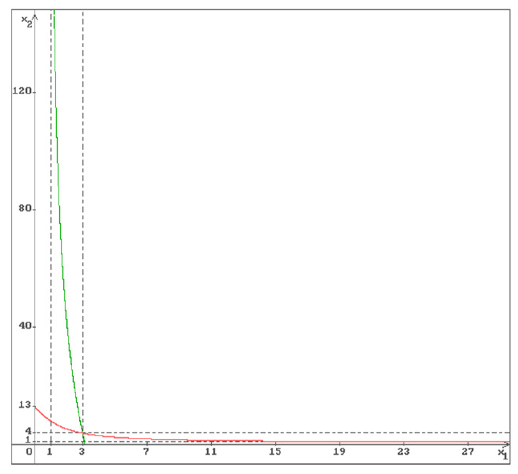
Figure 2.
The intersection point of the graphs of the functions (green) and (red) is the equilibrium .
Figure 2.
The intersection point of the graphs of the functions (green) and (red) is the equilibrium .
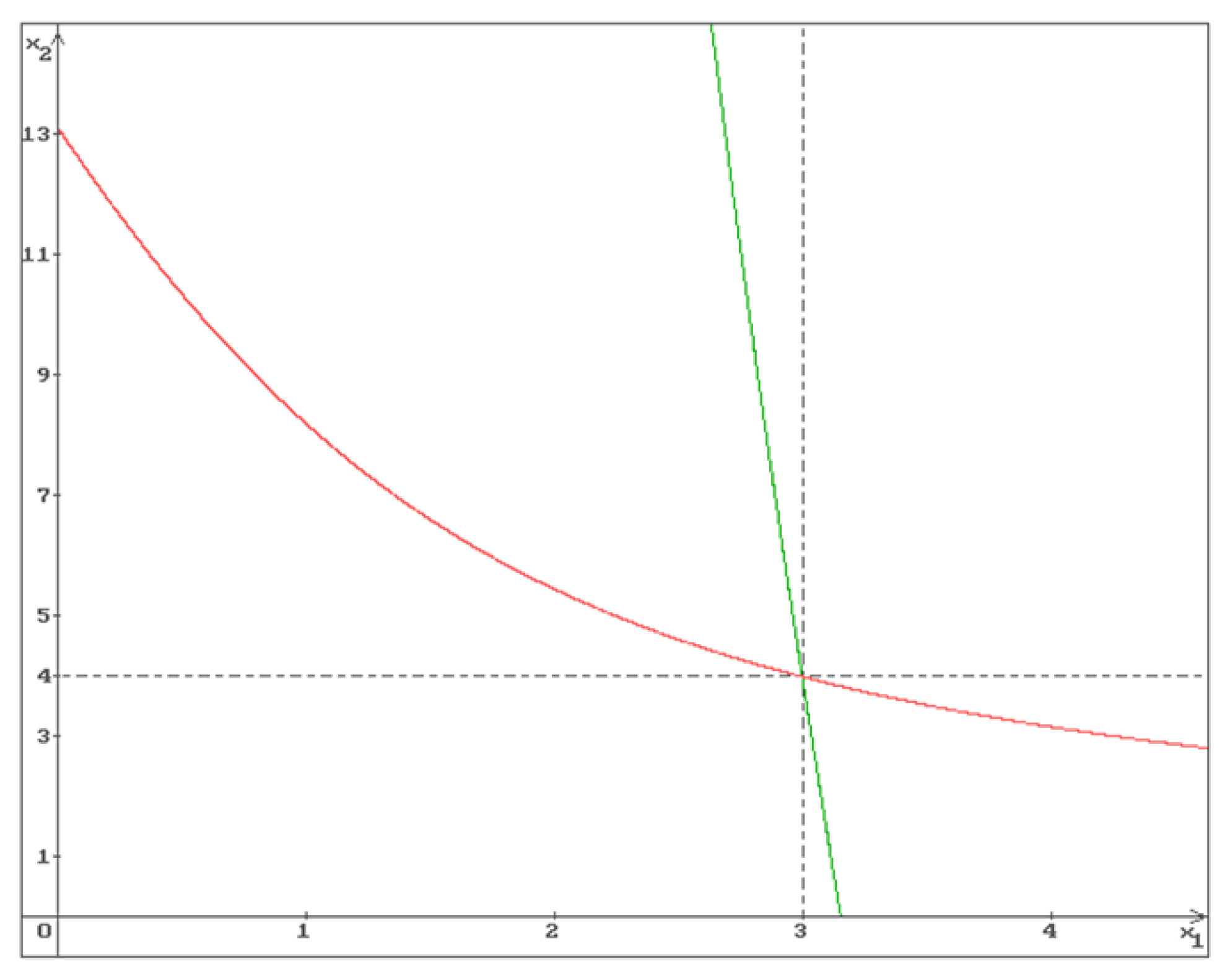
Figure 3.
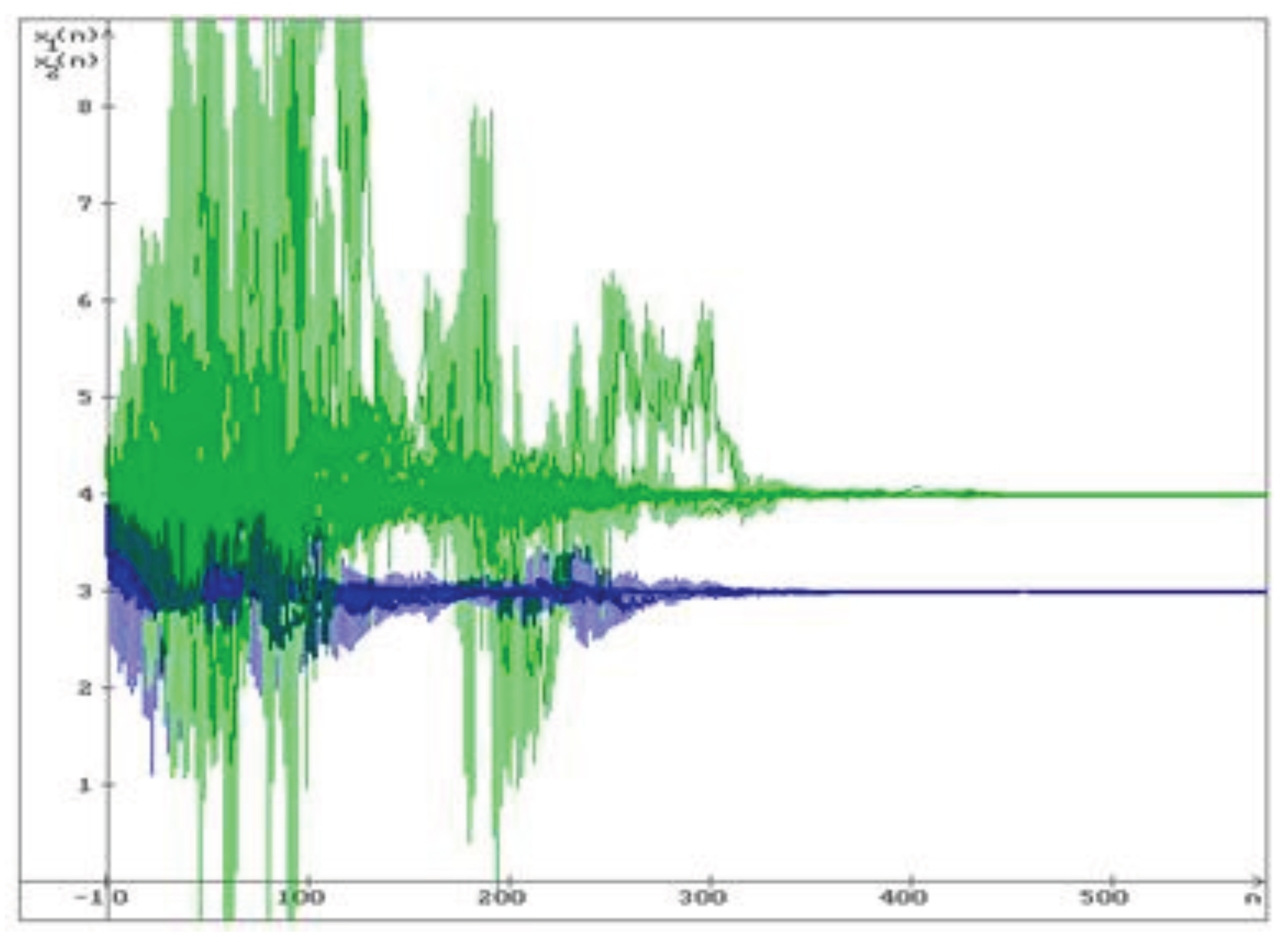
50 trajectories of the system (11) solution: (blue) and (green). The solution converges to the stable equilibrium .
Figure 3.
50 trajectories of the system (11) solution: (blue) and (green). The solution converges to the stable equilibrium .
Disclaimer/Publisher’s Note: The statements, opinions and data contained in all publications are solely those of the individual author(s) and contributor(s) and not of MDPI and/or the editor(s). MDPI and/or the editor(s) disclaim responsibility for any injury to people or property resulting from any ideas, methods, instructions or products referred to in the content. |
© 2025 by the authors. Licensee MDPI, Basel, Switzerland. This article is an open access article distributed under the terms and conditions of the Creative Commons Attribution (CC BY) license (http://creativecommons.org/licenses/by/4.0/).
Copyright: This open access article is published under a Creative Commons CC BY 4.0 license, which permit the free download, distribution, and reuse, provided that the author and preprint are cited in any reuse.


