
Submitted:
13 August 2025
Posted:
22 August 2025
You are already at the latest version
Abstract
During the last two decades, rational difference equations, in particular, rational bilinear difference equations, have become
very popular in research. In this paper the asymptotic properties of one rational bilinear difference equation are rst studied
under stochastic perturbations. It is assumed that stochastic perturbations are directly proportional to the deviation of the
current value of the equation solution from one of its equilibria (the zero or nonzero). Some conditions are obtained by which
the equilibrium under consideration is stable in probability or unstable. The obtained results are illustrated by numerical
simulation of solutions of the considered stochastic difference equation. It is noted, that the research method used here can be
applied to stability investigation of many other types of nonlinear difference equations with the order of nonlinearity higher
than one. Some directions for further development of research are proposed.
To readers attention some discussion about an unsolved problem of stabilization by noise for stochastic difference equations
is also proposed. This problem, well known already for more than 50 years for stochastic differential equations, has not yet
been solved until now for stochastic difference equations.
Keywords:
zero and nonzero equilibria
; stochastic perturbations
; stability in probability
; asymptotic mean square stability
; numerical simulation
; unsolved problem
1. Introduction
During the last two decades, rational difference equations, in particular, rational bilinear difference equations have become very popular in research (see, for instance, [1,2,3,4,5,6,7,8,9,10,11,12,13,14,15,16,17] and references therein). Various interesting results related to the solvability and stability of equations of this type are obtained. In particular, stability of the bilinear difference equation
with positive parameters and initial values , is studied in [7].
It is clear that, without loss of generality, one of the parameters in this equation can be equated to 1. Let . So, we will consider the bilinear difference equation
with positive and , .
Statement 1 If then the unique equilibrium of the Equation (1) is .
Statement 2 If then the zero solution of the Equation (1) is locally asymptotically stable.
Below, the bilinear difference Equation (1) is studied under stochastic perturbations that are directly proportional to the deviation of the current value of the solution of the stochastic bilinear difference equation under consideration from the zero or nonzero equilibrium of the Equation (1). To the best of author’ knowledge stochastic bilinear difference equations have not yet been considered.
Based on the obtained results, a hypothesis is proposed and discussed about the possibility of "stabilization by noise" for stochastic difference equations. The well-known effect of "stabilization by noise" for stochastic differential equations still has no analogue for stochastic difference equations. Here, this hypothesis is tested by numerical simulation and confirmed, but the formal proof of this hypothesis is still an unsolved problem.
1.1. Equilibria of the Equation (1)
Putting for , we obtain that the equilibrium of the Equation (1) is defined by the equation
It is clear that if
then only can be the equilibrium of the Equation (1) (that coincides with Statement 1).
From the other hand, by the assumption
each is a solution of the Equation (2) and , , is a solution of the Equation (1).
Remark 1.
Below stability of the zero and nonzero equilibria of the Equation (1) is investigated under stochastic perturbations.
2. Some Transformations of the Initial Equation
Let be a discrete time, , . Let be a basic probability space, , , be a nondecreasing family of -algebras, be the expectation, be a sequence of -adapted mutually independent identically distributed random variables such that , , [18].
Note that via Remark 1 by the condition (4) and the Equation (1) has the equilibrium . Let us assume that the Equation (1) is exposed to stochastic perturbations that are directly proportional to the deviation of the solution from the equilibrium , i.e., the Equation (1) takes the form of the stochastic difference equation [18]
where is a constant. By that the solution of the Equation (1) is also the solution of the Equation (5).
Remark 2.
Lemma 1.
3. Stability
Consider the scalar stochastic difference equation [18]
where a, b, are constants and is described above.
Definition 1.
Definition 2.
The zero solution of the Equation (10) is called:
- mean square stable if for each there exists a such that , , for any initial function such that ;
- asymptotically mean square stable if it is mean square stable and for each initial function such that the solution of the Equation (10) satisfies the condition .
Remark 3.
It is clear that stability of the equilibrium of the Equation (5) is equivalent to stability of the zero solution of the Equation (6). It is known [18] that the investigation of stability in probability of the zero solution of a nonlinear stochastic difference equation with an order of nonlinearity higher than one can be reduced to the investigation of asymptotic mean square stability of the zero solution of the linear part of this equation. So, to get conditions for stability in probability of the equilibrium of the nonlinear stochastic difference Equation (5) it is enough to get conditions for asymptotic mean square stability of the zero solution of the linear stochastic difference Equation (7) that is the linear part of the nonlinear difference Equation (6).
Remark 4.
Lemma 2.
Lemma 3.
The inequalities
are the necessary and sufficient conditions for asymptotic mean square stability of the zero solution of the Equation (10).
Remark 5.
Theorem 1.
Proof.
From the condition (3) it follows that by the condition (13) the Equation (5) has the equilibrium only. Note also that
So, for the Equation (7) the condition (11) takes the form (13). Via Lemma 2 it means that by the condition (13) the equilibrium of the Equation (7) is asymptotically mean square stable and via Remark 3, the equilibrium of the Equation (5) is stable in probability. The proof is completed. □
Remark 6.
Note that the conditions (12) for the Equation (7) take the form
Thus, the inequalities (14) are necessary and sufficient conditions for asymptotic mean square stability of the zero solution of the Equation (7) and, therefore, via Remark 3, sufficient conditions for stability in probability of the solution of the Equation (5).
Remark 7.
Remark 8.
Note that in all examples below for numerical simulation of solutions of the Equation (5) the random value is used in the form , where η is a random value uniformly distributed on the interval with and . So, , .
Example 1.
Put , , , . The condition (13) holds: . Besides, the conditions (13) and (14) give respectively and . Via Theorem 1 the zero solution of the Equation (5) with is stable in probability. In Figure 1 500 trajectories (blue) of the solution of the Equation (5) are shown with the initial conditions , , all trajectories converge to zero. The red line corresponds to the deterministic case, i.e., .
Example 2.
Put now with the same values of all other parameters as in Example 1. The conditions (13) and (14) do not hold. In Figure 2 500 trajectories (blue) of the solution of the Equation (5) with are shown with the initial conditions , . The zero solution is unstable and the trajectories fill the whole space. The red line corresponds to the deterministic case, i.e., .
Example 3.
Put , , , , . Wherein , therefore, the condition (4) holds, the conditions (13) and (14) do not hold. In Figure 3 the red straight corresponds to the constant solution , , 500 trajectories (blue) of the solution of the Equation (5) are shown with the initial conditions , . The solution is unstable, so, the trajectories fill the whole space.
4. About One Unsolved Problem of Stabilization by Noise
More than 50 years ago Khasminskii shows [24] that unstable by the conditions and the zero solution of the differential equation
becomes stable by the presence of a big enough level of noise. More exactly, by the condition
so-called "stabilization by noise" occurs and the zero solution of the Equation (15) becomes stable in probability.
Really, let L be the generator [20,24,25] of the stochastic differential Equation (15). For the Lyapunov function it has the form
So, via (16) for the Lyapunov function
we have
From the obtained condition it follows that the zero solution of the Equation (15) is stable in probability [20,24].
As it is noted in [26] any similar result for the stochastic difference Equation (10) is absent until now even in the case . But the following example shows that the effect of stabilization by noise can take a place for difference equations too.
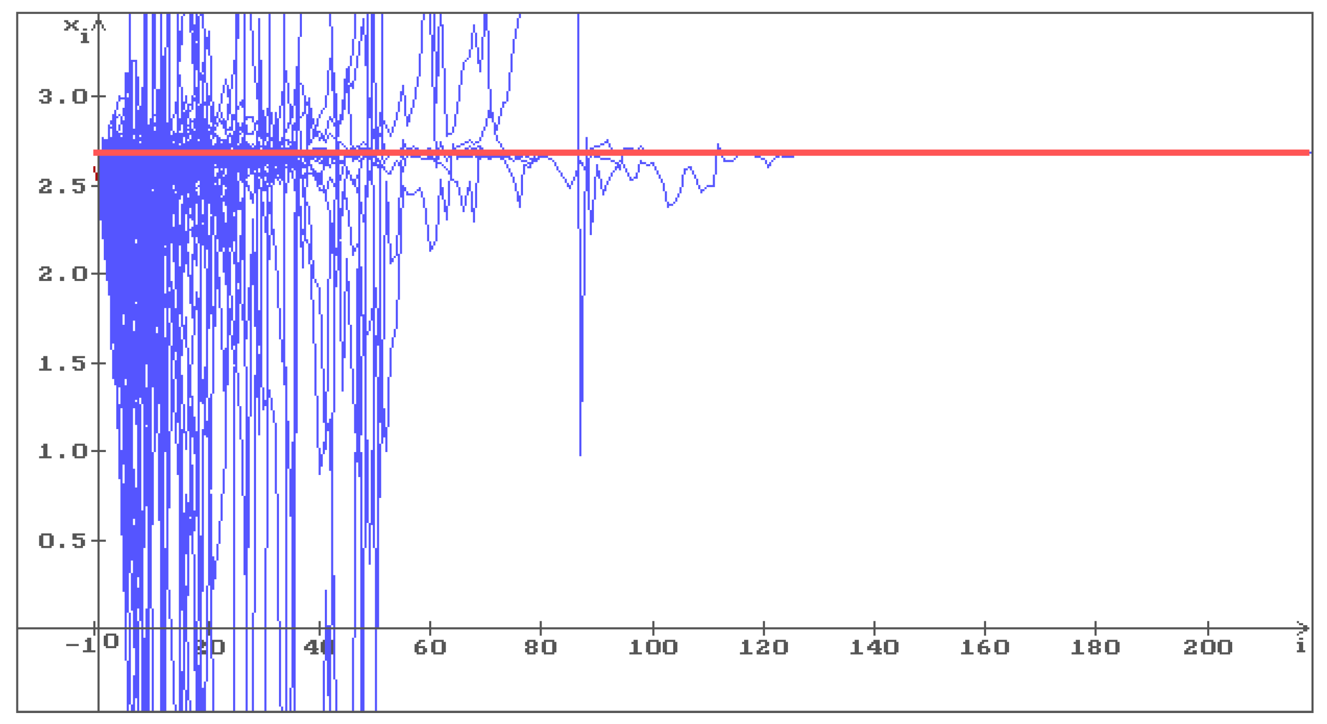
Example 4.
Consider Example 3 again with and the same values of all other parameters. In Figure 4 one can see that all 500 trajectories converge to the solution of the Equation (5). Putting , i.e., increasing once more the level of noise, we obtain (see Figure 5) that all 500 trajectories converge to the solution of the Equation (5) faster than in Figure 4. So, the solution of the Equation (5), that is unstable by the small level of noise (Figure 3, ), becomes stable by increasing the level of noise.
Thus, the Hypothesis about stabilization by noise for stochastic difference equations may well take a place. However, the proof of this Hypothesis is currently an unsolved problem.
5. Conclusions
In conclusion, one would like to note that the study of the asymptotic properties of a bilinear difference equation under stochastic perturbations is carried out here for the first time, and that the research method used here can be extended to the following natural directions of research development:
1) Bilinear difference equations of other forms, for instance, obtained from this one
using different combinations of plus and minus. In each case, one can expect the appearance of new features of the solution behavior.
2) Different mathematical models in various applications, described by nonlinear stochastic difference equations of a more complex form.
3) Formulate and prove for difference equations a statement similar to Khasminsky’s statement about "stabilization by noise", which has been well known in the theory of stochastic differential equations for more than 50 years, but still has no analogue for stochastic difference equations.
Funding
This research received no external funding.
Institutional Review Board Statement
Not applicable.
Informed Consent Statement
Not applicable.
Data Availability Statement
Not applicable.
Conflicts of Interest
The author declares no conflict of interest.
References
- Abo-Zeid, R.; Kamal, H. On the solutions of a third order rational difference equation. Thai Journal of Mathematics, 2020, 18(4), 1865-1874.
- Aloqeili, M. Dynamics of a rational difference equation. Applied Mathematics and Computation, 2006, 176(2), 768-774. [CrossRef]
- Camouzis, E.; Ladas, G.; Voulov, H.D. On the dynamics of . Journal of Difference Equations and Applications, 2003, 9(8), 731-738.
- Chatterjee, E.; Grove, E.A.; Kostrov, Y.; Ladas,G. On the trichotomy character of . Journal of Difference Equations and Applications, 2003, 9(12), 1113-1128.
- Cinar, C. On the positive solutions of the difference equation . Applied Mathematics and Computation, 2004, 156, 587-590 [CrossRef]
- Elabbasy, E.M.; EI-Metwally, H.; Elsayed, E.M. On the difference equations . Advances in Difference Equations, 2006, (2006), Article ID 82579, 1-10.
- Elsayed, E.M. Qualitative behavior of a rational recursive sequence. Indagationes Mathematicae, N.S, 2008, 19(2), 189-201.
- Grove, E.A.; Kulenovic, M.R.S.; Ladas, G. Progress report on rational difference equations. Journal of Difference Equations and Applications, 2004, 10(13-15), 1313-1327.
- Halim, Y.; Touafek, N.; Yazlik, Y. Dynamic behavior of a second-order nonlinear rational difference equation. Turkish Journal of Mathematics, 2015, 39(6), 1004-1018. [CrossRef]
- Ibrahim, T.F.; Touafek, N. On a third order rational difference equation with variable coefficients. Dynamics of Continuous, Discrete and Impulsive Systems, Series B: Applications & Algorithms, 2013, 20(2), 251-264.
- Papaschinopoulos, G.; Stefanidou, G. Asymptotic behavior of the solutions of a class of rational difference equations. International Journal of Difference Equations, 2010, 5(2), 233-249.
- Stevic, S. On the system . Applied Mathematics and Computation, 2013, 219, 4526–4534. [Google Scholar]
- Stevic, S. Representations of solutions to linear and bilinear difference equations and systems of bilinear difference equations. Advances in Difference Equations. 2018, Vol. 2018, Article No.474, 21 pages.
- Stevic, S.; Diblík, J.; Iricanin, B.; Smarda, Z. On a solvable system of rational difference equations. Journal of Difference Equations and Applications, 2014, 20(5–6), 811-825.
- Stevic, S., Iricanin, B., Kosmala, W., Smarda, Z. Note on a solution form to the cyclic bilinear system of difference equations. Applied Mathematics Letters, 2021, 111, 106690.
- Taskara, N.; Tollu, D.T.; Yazlik, Y. Solutions of rational difference system of order three in terms of Padovan numbers. Journal of Advanced Research in Applied Mathematics, 2015, 7(3), 18-29.
- Yazlik, Y. On the solutions and behavior of rational difference equations. Journal of Computational Analysis and Applications, 2014, 17(3), 584-594.
- Shaikhet, L. Lyapunov functionals and stability of stochastic difference equations. Springer Science & Business Media: London, UK, 2011.
- Beretta, E.; Kolmanovskii, V.; Shaikhet, L. Stability of epidemic model with time delays influenced by stochastic perturbations. Mathematics and Computers in Simulation (Special Issue "Delay Systems"), 1998, 45(3-4), 269-277. https://www.sciencedirect.com/science/article/pii/S0378475497001067. [CrossRef]
- Shaikhet, L. Lyapunov functionals and stability of stochastic functional differential equations. Springer Science & Business Media: Berlin/Heidelberg, Germany, 2013.
- Shaikhet, L. About one method of stability investigation for nonlinear stochastic delay differential equations. International Journal of Robust and Nonlinear Control, 2021, 31(8), 2946-2959, https://onlinelibrary.wiley.com/doi/10.1002/rnc.5440.
- Shaikhet, L. Some generalization of the method of stability investigation for nonlinear stochastic delay differential equations. MDPI, Symmetry, 2022, 14(8), 1734, 1-13, https://www.mdpi.com/2073-8994/14/8/1734/pdf. [CrossRef]
- Shaikhet L. About stability of nonlinear stochastic differential equations with state-dependent delay. MDPI, Symmetry, 2022, 14(11), 2307, 1-12, https://www.mdpi.com/2073-8994/14/11/2307/pdf.
- Khasminskii, R.Z. Stochastic stability of differential equations; Springer: Berlin, Germany, 2012 (in Russian, Moscow, Nauka, 1969).
- Gikhman, I.I., Skorokhod, A.V. Stochastic Differential Equations; Springer: Berlin, Germany, 1972.
- Shaikhet, L. Some unsolved problems in stability and optimal control theory of stochastic systems. Special Issue "Models of Delay Differential Equations - II", MDPI, Mathematics, 2022, 10(3), 474, 1-10. [CrossRef]
Figure 1.
500 trajectories (blue) of the solution of the Equation (5) with , , b=, , , , . The red line corresponds to the deterministic case, i.e. .
Figure 1.
500 trajectories (blue) of the solution of the Equation (5) with , , b=, , , , . The red line corresponds to the deterministic case, i.e. .
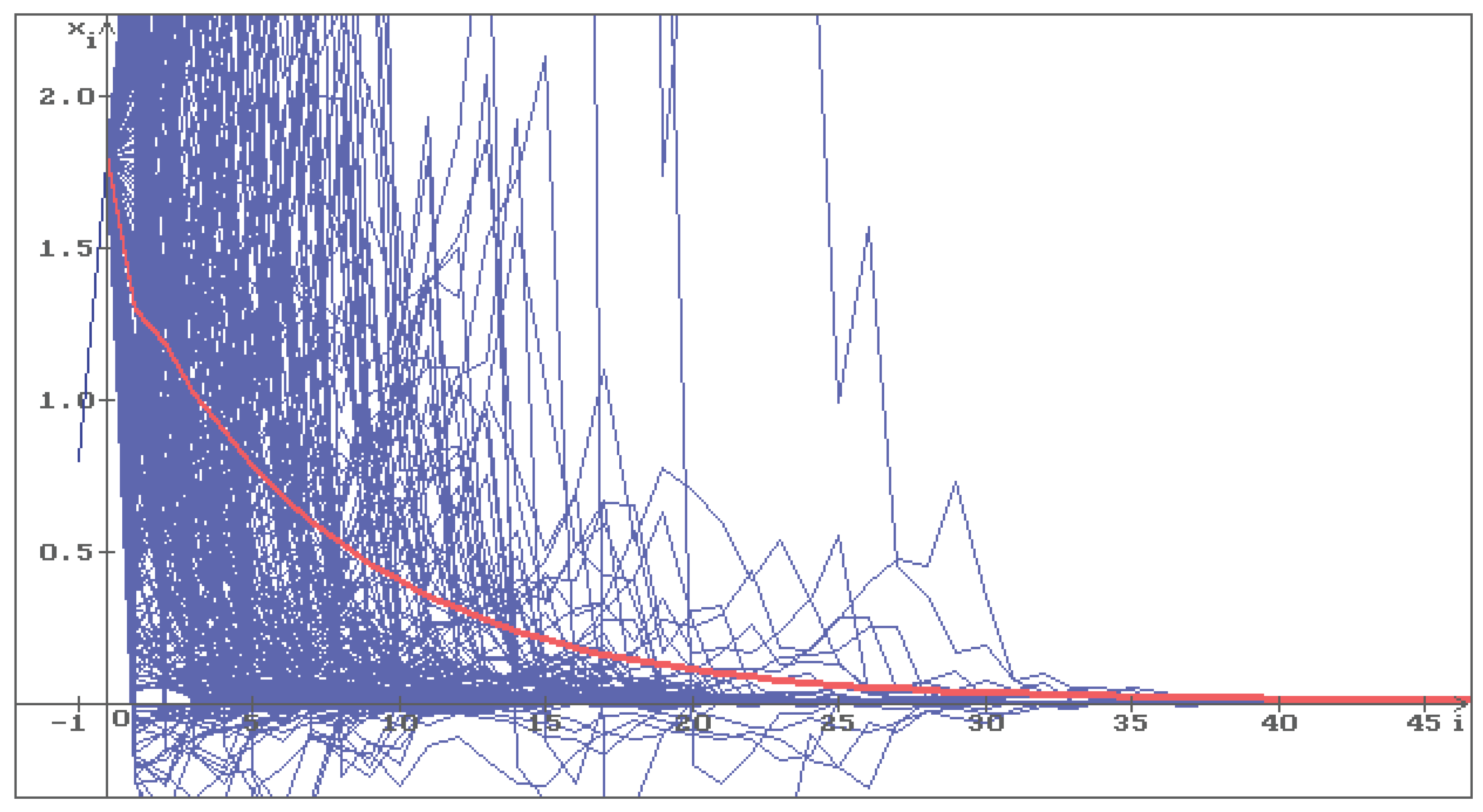
Figure 2.
500 trajectories (blue) of the solution of the Equation (5) with , , b=, , , , . The red line corresponds to the deterministic case, i.e.
Figure 2.
500 trajectories (blue) of the solution of the Equation (5) with , , b=, , , , . The red line corresponds to the deterministic case, i.e.
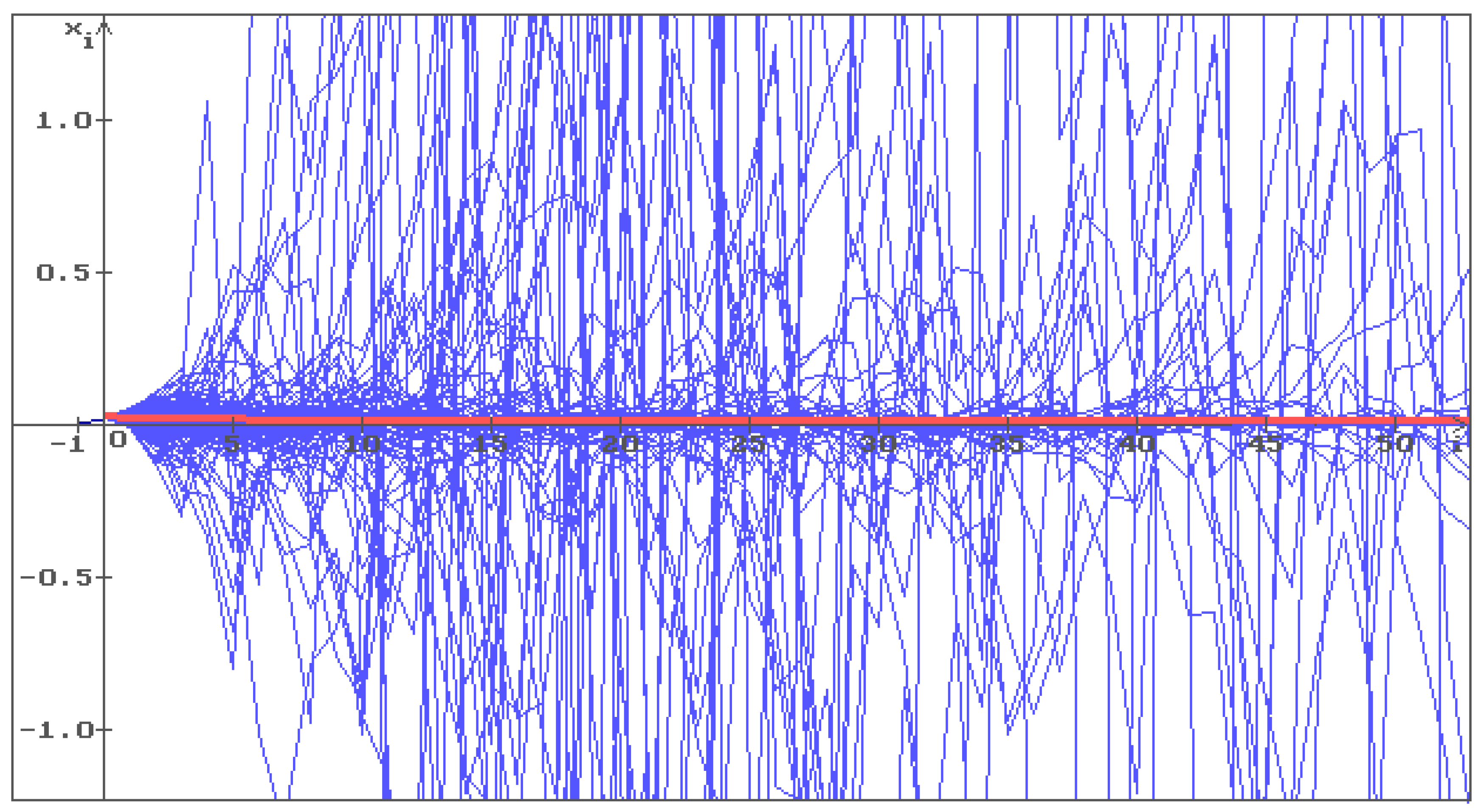
Figure 3.
500 trajectories (blue) of the solution of the Equation (5) with , , b=, , , , . The red straight corresponds to the constant solution , ,
Figure 3.
500 trajectories (blue) of the solution of the Equation (5) with , , b=, , , , . The red straight corresponds to the constant solution , ,
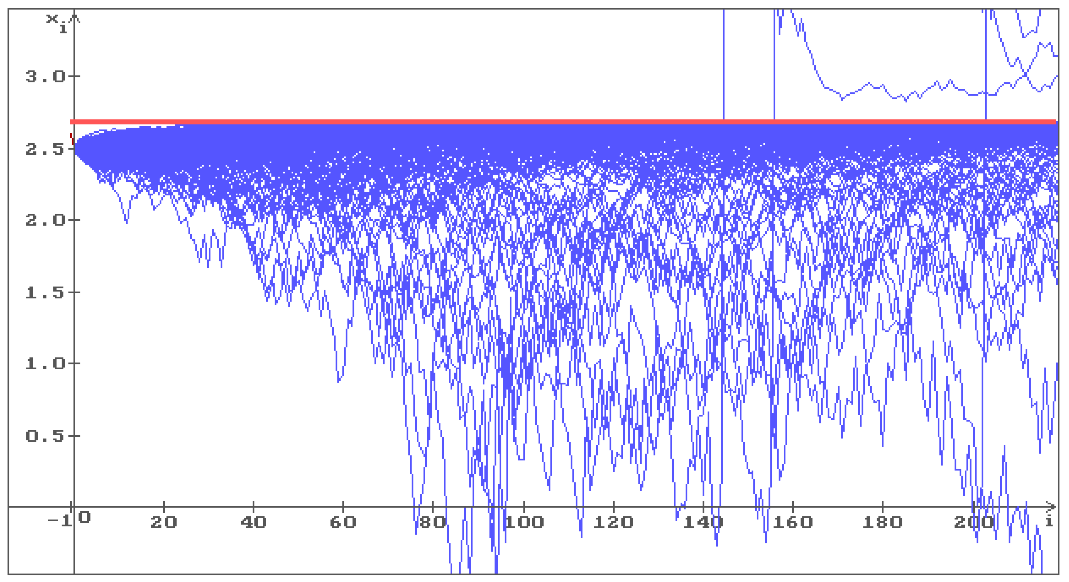
Figure 4.
500 trajectories (blue) of the solution of the Equation (5) with and the same values of all other parameters as in Figure 3.

Disclaimer/Publisher’s Note: The statements, opinions and data contained in all publications are solely those of the individual author(s) and contributor(s) and not of MDPI and/or the editor(s). MDPI and/or the editor(s) disclaim responsibility for any injury to people or property resulting from any ideas, methods, instructions or products referred to in the content. |
© 2025 by the authors. Licensee MDPI, Basel, Switzerland. This article is an open access article distributed under the terms and conditions of the Creative Commons Attribution (CC BY) license (http://creativecommons.org/licenses/by/4.0/).
Copyright: This open access article is published under a Creative Commons CC BY 4.0 license, which permit the free download, distribution, and reuse, provided that the author and preprint are cited in any reuse.


