
Submitted:
07 May 2025
Posted:
08 May 2025
You are already at the latest version
Abstract
The spectrum modeling of emission spectrum of yellow phosphor YAG:Ce3+ is an important role in investigation the optical properties of white light. We proposed and demonstrated a novel solution for modeling the emission of yellow phosphor YAG:Ce3+ by using the PYTHON software. The emission curve is mathematically described by using the Gaussian function. This mathematical model is simulated by progaming in PYTHON. The similarity between the simulation and experimental results are compared by normalized cross correlation (NCC) algorithm. All NCCs show high values largers than 99.5% which indicates the accuracy and reliability of the model. The proposed model is interesting and meaningful for emission spectrum modeling uisng the PYTHON software programming. Its appliactions offers a blend of cost-efficiency, speed, and comprehensive insight while allowing for extensive control and customization. The combination of these advantages positions this method as a powerful tool in materials science, lighting technology, and display.
Keywords:
PYTHON spectrum modeling
; PYTHON yellow phosphor
; PYTHON normalized cross correlation
1. Introduction
Light emitting diodes (LED) based solid state lighting has become the dominant light source due to its advantages of energy saving, color vividness, compact size, high luminous efficiency, and environment friendly due to free mercury (Schubert, 2005; Narendran et.al., 2005; Schubert, 2006; Sun et.al., 2022; Nguyen et al., 2023). The most popular method in industrial lighting to generate white light is using a blue LED die covered with yellow phosphor YAG:Ce3+ (Nguyen et al., 2025). The type of yellow phosphor has a broad emission band (e.g., wavelength range from 500 nm to 750 nm) which is a high overlapping level to the human eye’s sensitivity curve (Xie et al., 2011) [7]. These unique characteristics help generate a high luminous efficiency while saving energy. Figure 1 illustrates the white light mixing process with the yellow and blue light combination. The blue light from blue LED excitation sources pump to the yellow phosphor will be absorbed by the yellow phosphor. The amount of absorbed blue light will be converted to yellow light. The unabsorbed blue light is transmitted through the phosphor layer and mixed with converted yellow light. The mixture of light causes a white feeling in the perceving of humans’s eyes. Under the excitation of blue light, electrons in the (5s25p6)4f 1 ground state are moved up to the (5s25p6)5d1 excited state. Through a down-conversion process, the down-conversion of electrons between the (5s25p6)5d1 excited state and (5s25p6)4f 1 ground state releases the energy as a broad emission band in the yellow light region of the visible region (Nguyen et al., 2024; Yang et.al., 2018). As a result, an asymmetry band of the emission spectrum of yellow light is obtained as shown in Figure 2.
The simulation of the emission spectrum has attracted much attention. J. de Bonfils et al. reported that a simplified inactive rare-earths doped nuclear waste glasses have been obtained by molecular dynamics (MD) simulation in order to investigate the local structure around the rare-earth by luminescence studies. MD calculations were performed with modified Born–Mayer–Huggins potentials and three body angular terms representing Coulomb and covalent interactions. The simulated emission spectra are obtained by convolution of all the Eu3+ ions contributions. A comparison with the experimental data issue from fluorescence line narrowing and microluminescence spectroscopies allowed us not only to validate the simulation of luminescence spectra from simulated environments, but also to confirm the presence and the identification of two major Eu3+ sites distribution in the nuclear glasses thanks to spectra-structure correlations (Bonfils et al. 2008). Koryukina et al. simulated the emission spectra of Ne and Ar atoms in an inductive discharge. The influence of the alternating electric field generated by this discharge on the spectral characteristics of light sources is studied. Based on the results of calculations, the regularities in the behavior of spectra characteristics of Ne and Ar atoms in the electric field have been revealed. Practical applications of the simulation results are considered (Koryukina et al. , 2017). Avtaeva et al. developed a modeling of the Sulfur emission in the asymmetric pulse dielectric barrier discharge. The asymmetric pulse-periodic dielectric barrier discharge (DBD) in a mixture of argon with sulfur vapor exhibits the emission spectrum of the discharge with intense bands of S2 molecules in the visible region. The modeling of the discharge characteristics in Ar–S2 mixture within the 1D fluid model is presented showing that during a voltage pulse of 150 ns, an electropositive plasma is formed in the entire discharge gap with the electron number density reaching values above 1,5.1018 m−3 at the maximum under the mean electron energy of about 3 eV. The high electron number density during the current pulse leads to efficient excitation of sulfur dimers, as a result, their radiative efficiency during the voltage pulse reaches approximately 4%. The discharge is considered as promising one for creating radiation source in visible region of spectrum (Avtaeva , 2023). Xie et al. investigated a secondary electron emission model for photo-emission from metals in the vacuum ultraviolet. The two secondary electron emission models for photoelectric energy distribution curves, absolute quantum efficiency, and the mean escape depth of photo-emitted electrons of metals have been developed. The proposed models are developed based on the density of states and the theories of photo-emission in the vacuum ultraviolet. The mean probability that an internal photo-emitted electron escapes into vacuum upon reaching the emission surface of the metal, and the mean energy of photo-emitted electrons measured from vacuum are ultized in this emission modeling (Xie et al., 2022). Suryan Sivadas et al. reported that the atomic emission spectroscopy is a potential tool for qualitative and quantitative elemental analysis of multi-element materials. The emission spectrum is composed of the characteristic lines of the constituent species, and their intensities are proportional to the population of their energy states and transition probability. The authors have simulated the emission spectrum of copper-tin-zinc alloys under typical laser-induced plasma conditions. Spectra are generated for varying temperatures, electron density, and compositions and show variations based on these parameters. This simulation provides a simple and convenient way to perform laser-induced breakdown spectroscopy applications on any alloy sample (Suryan Sivadas, 2022). Vu et al. have proposed and demonstrated a precision optical model for red light-emitting diodes and applied this model to improve the color rendering index of phosphor-converted white light-emitting diodes. The inherent asymmetry properties of red light emission bands have been conquered and effectively modeled. The accuracy of the red light optical model is confirmed with the experimental spectrum and verified by normalized cross-correlation. In an application, the Gaussian functions-based mathematical model is applied to simulate the emission spectrum of white light with and without adding red light. The supplement of red light is optimized to improve the CRI index of output white light. As a result, the color performance of white LEDs is improved when the CRI value significantly increases from 79 to 93 by adding an optimized amount of red light. The effect of added red light on white-LEDs properties has been investigated including correlated color temperature, output lumen, CIE-chromaticity coordinates, and luminous efficiency of radiation. In addition, the effect of adding red light on color rendering quality of output white light is studied with the IES TM 30–18 application (Vu et.al., 2025). Nguyen has reported a mathematical model for emission spectrum modeling that is simple, easy to use, understandable, and applicable. The model can be applied to design an emission spectrum using LED, studying the optical and color performance of the emitted white light spectrum. This efficient method is helpful for researchersworking in the solid-state lighting (SSL) field, spectrum design for light sources, and optimizingthe optical and electrical performanceofany specificdesired light source (Nguyen, 2023). Vo et al. developed an efficient optical model for simulating the white light spectrum design with high color performance. The optical model began with experimental data collection, simulation with the mathematical model using Gaussian functions, and verifying the similarity between simulation and experiment. In application, the model is applied to study the effect of red light on the optical properties of the generated white light spectrum. The obtained results indicate that the established model is helpful for the solid-state lighting application to fabricate a light source that can emit white light with high optical performance (Vo et al., 2024). Nguyen et al. developed an optical model for green phosphor pumped by ultraviolet (UV) laser. The model began by defining an efficient mathematical model to describe the emission of the UV band and green light. Next, the data of peak emission wavelength, the width of the emission band, and the emission wavelength range are extracted from the measurement of the emission spectrum of green phosphor pumped by a UV laser. These parameters are put in the mathematical model to simulate the emission spectrum of green phosphor pumped by a UV laser. Finally, the optical model is verified with experimental measurements. The similarity of simulation and experiment is quantified using a normalized cross-correlation algorithm (Nguyen et al., 2025).
Spectrum modeling can help to predict the optical and color properties of output light (Nguyen, 2023; Chien et.al., 2007; Sun et al., 2008). Traditional methods use Excel to calculate the power spectrum distribution of white light (Vo et al., 2024; Nguyen et al., 2025). This method is simple and does not require advanced software, however, it is time-consuming. The other method to simulate the SPD is using Matlab. This method is fast and convenient for those who are familiar with Matlab. Along with the development of information technology, many programming languages are launched such as C, C++, and Python. This leads to a requirement to apply these new programming languages in scientific and technology-related works. Python has become preferred and widely used due to it being an open-source programming language (Smet et al., 2019). The application of Python in the solid-state lighting field is still in the beginning stages. Thus, it motivated us to conduct this research to promote the development of this field by using the PYTHON programing language.
In this paper, we studied and verified a novel method to simulate the yellow phosphor’s emission spectrum. The emission is described by the Gaussian function which is simulated effectively by programming in PYTHON. Emission spectra with different bandwidths are simulated easily. The similarities between the simulation and experimental results are compared by the normalized cross-correlation (NCC) algorithm. The proposed model is clear evidence to prove that PYTHON software programming is an interesting and meaningful tool in the solid-state lighting field.
2. Methodology
Figure 3a shows the asymmetric band of the emission spectrum of yellow light. To simplify the simulation, the detailed analysis of the emission curve of the yellow emission spectrum is described as follows. At the peak emission wavelength position of the yellow band, the emission band is divided into two parts by a normal to the wavelength axis. These two halves of a bell shape as shown in Figure 3b,c. These two bell shapes have the same peak emission wavelength but have different full widths at haft maximum (FWHM). Based on these characteristics, the simulation of the asymmetric band of the emission spectrum of yellow light as shown in Figure 3a is described as follows. To simulate the halves of the curve of the bell shape with FWHM 1, the wavelength range is from the value of wavelength 1 to peak wavelength. Half of the curve of the bell shapes with FWHM 2, the wavelength range is from the value of peak wavelength to wavelength 2.
In terms of mathematical representation, the emission curve with the bell shape is described by Gaussian functions,
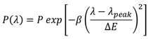
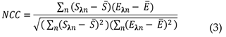
In validation the model, the beta value which has the highest level of overlapping of the simulated and experimental spectrum should be defined. The precise comparison is conducted through quantitative evaluation using the normalized cross correlation (NCC) algorithm (Sun et al., 2006; Nguyen et al. 2024). The similarity between simulation and experiment spectrum curves is quantitatively evaluated based on the value of NCC (e.g., the value of 100 for NCC means the complete similarity between the simulated and experimental spectrum). The mathematical expression of the NCC algorithm is described as follows (Sun et al., 2006; Nguyen et al. 2024).
3. Simulation Spectrum of Yellow Emission Using PYTHON
To simulate and visualize the emission spectrum of yellow light using Python, we will utilize libraries such as NumPy and Matplotlib. The emission spectrum of yellow light can be approximated with a Gaussian distribution centered around the wavelength of yellow light, which typically ranges from about 400 nm to 800 nm in visble light. Based on the mathematical equation (1) and Python programming, the simulation spectrum of yellow emission is obtained as shown in Figure 4. The codes for the simulation spectrum of yellow emission using PYTHON are shown as follows
-
# Import the libraries used in this scriptimport numpy as npimport matplotlib.pyplot as pltimport matplotlib.ticker as tickerimport pandas as pd# File pathfile_path = ‘/kaggle/input/yellow-phosphor-spectrum/normalized-experimental-spectrum-of-yellow-phosphor-PLP1279.xlsx’# Read datadata = pd.read_excel(file_path)# Extract data from the filelambda_experimental_values = data[‘Wavelength’].valuesexperimental_data = data[‘normalized Spectral flux’].values#Check the data in filetry:lambda_experimental_values = data[‘Wavelength’].dropna().valuesexperimental_data = data[‘normalized Spectral flux’].dropna().valuesexcept KeyError as e:print(f”Error: Missing expected column in data: {e}”)# Main parametersP = 1 # Emission band powerlambda_peak = 564 # Peak emission wavelengthlambda_mid = 564 # Wavelength dividing the emission band into two parts# Beta values for simulationbetas = [2.6, 2.7, 2.8, 2.9, 3.0, 3.1]beta_step_1 = [1, 2, 3, 4, 5, 6, 7]beta_step_05 = [1.5, 2, 2.5, 2.8, 2.85, 2.9, 3, 3.5, 4, 4.5, 5, 5.5, 6, 6.5, 7]# Simulate and plot the phosphor emission spectrum using a Gaussian functionplt.figure(figsize=(10, 6))for beta in beta_step_1:P_lambda_left = P * np.exp(-beta * ((lambda_experimental_values[lambda_experimental_values <= lambda_mid] - lambda_peak) / 52) ** 2)P_lambda_right = P * np.exp(-beta * ((lambda_experimental_values[lambda_experimental_values > lambda_mid] - lambda_peak) / 174) ** 2)P_lambda = np.concatenate([P_lambda_left, P_lambda_right])plt.plot(lambda_experimental_values, P_lambda, label=f’Simulation with Beta={beta}’, linewidth=5)# Plot the phosphor emission spectrumplt.xlabel(‘Wavelength (nm)’, fontsize=12, fontweight=‘bold’)plt.ylabel(‘Normalized Flux (a.u.)’, fontsize=12, fontweight=‘bold’)plt.title(‘Simulated Spectrum (Beta Step=1)’, fontsize=14, fontweight=‘bold’)plt.legend()plt.grid(alpha=0.5)plt.tight_layout()plt.show()# There are seven beta values (in beta_step_1 list) used to plot the simulation spectrum
Running the code will generate a graph displaying a Gaussian curve peaking at 580 nm, representing the simulated emission spectrum of yellow light. Adjust the values of “lambda_peak” and “Beta” to simulate different shapes of yellow emission. Figure 4 shows the simulated emission spectrum under different values of beta constant. Different values of beta including 1, 2,3, 4, 5, 6, and 7, respectively were used in the simulation. The result indicates that the width of the emission band is proportional to the used value of beta.
Verifying the emission spectrum modeling involves comparing the simulated data generated by the model with experimental data, assessing the accuracy of the model, and ensuring it behaves as expected under various conditions. A basic approach to verify the emission spectrum modeling using Python can include these steps for verification. Firstly, it is necessary to ensure that the model accurately represents the physical phenomena of the yellow phosphor emission. This includes checking the parameters of the Gaussian functions or other mathematical representations used in the model. Secondly, Compare with Experimental Data. By obtaining experimental data for the yellow phosphor’s emission spectrum with a spectrometer or from the literature. The simulated emission spectrum is plotted against the experimental data for visual comparison. Next, statistical analysis should be conducted using measures like R-squared, Root Mean Square Error (RMSE), or other statistical techniques to quantify the model’s accuracy in predicting the experimental data. It is important to find out the value of the beta constant to have the best match between simulation and experiment results. For that purpose, different values of the beta constant were used in the simulation to simulate the corresponding emission spectrum. Then this simulated spectrum is compared to the experimental spectrum by overlapping them in the same figure. The codes for conducting these purposes in PYTHON are shown as follows.
-
# Function calculates the value of NCCdef calculate_ncc(simulated, experimental):S_mean = np.mean(simulated)E_mean = np.mean(experimental)numerator = np.sum((simulated - S_mean) * (experimental - E_mean))denominator = np.sqrt(np.sum((simulated - S_mean) ** 2) * np.sum((experimental - E_mean) ** 2))return (numerator / denominator) * 100 # Return NCC as a percentage# Plot six phosphor emission spectra corresponding to different beta valuesfig, axes = plt.subplots(2, 3, figsize=(14, 7)) #Create figure with two rows and three columnsx_ticks = np.linspace(450, 900, 10)y_ticks = np.linspace(0, 1, 6)ncc_values = [] # Initial an empty list for ncc_valuesfor i, beta in enumerate(betas):# Compute P(lambda) for two regionsP_lambda_1 = P * np.exp(-beta * ((lambda_experimental_values[lambda_experimental_values <= lambda_mid] - lambda_peak) / 52) ** 2)P_lambda_2 = P * np.exp(-beta * ((lambda_experimental_values[lambda_experimental_values > lambda_mid] - lambda_peak) / 174) ** 2)P_lambda = np.concatenate([P_lambda_1, P_lambda_2])# Compute NCC for each beta (in betas list)ncc = calculate_ncc(P_lambda, experimental_data)ncc_values.append(ncc) #Append value to ncc_valuesprint(f’NCC for Beta={beta}: {ncc:.3f}%’)# Select subplot and plotax = axes[i // 3, i % 3]ax.plot(lambda_experimental_values, experimental_data, ‘k-‘, label=‘Normalized Experimental Data’, linewidth=3)ax.plot(lambda_experimental_values, P_lambda, ‘r-‘, label=f’Simulation with Beta={beta} (NCC={ncc:.3f}%)’, linewidth=3)# Configure axesax.set_xticks(x_ticks)ax.set_yticks(y_ticks)ax.set_xticklabels(x_ticks, rotation=45, ha=‘right’) ax.xaxis.set_major_formatter(ticker.StrMethodFormatter(‘{x:.0f}’))ax.set_title(f’Beta = {beta}’)ax.set_xlabel(‘Wavelength (nm)’)ax.set_ylabel(‘Normalized P(λ) (a.u.)’)ax.legend()plt.tight_layout()plt.show()# There are six different plots and corresponding NCC values for six different beta values. Each plot includes one simulated spectrum and one experimental spectrum.
Figure 5.
Comparison between simulation at different values of beta and experiment spectrum.
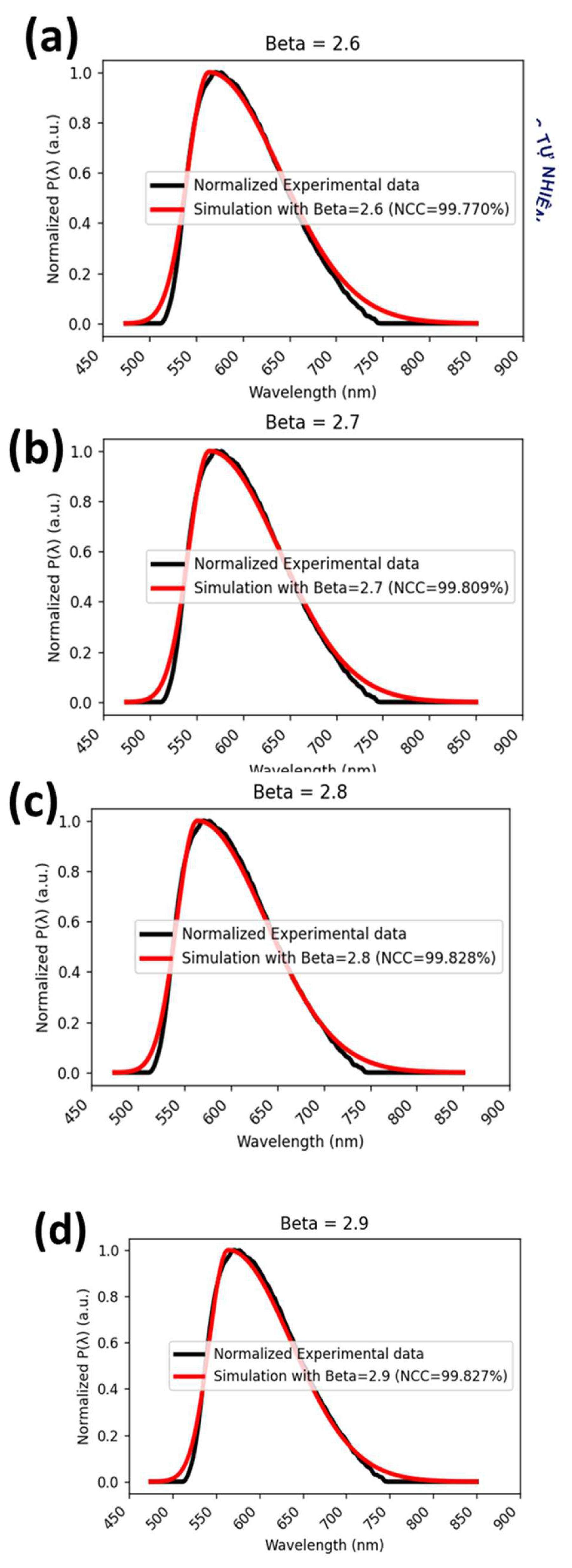
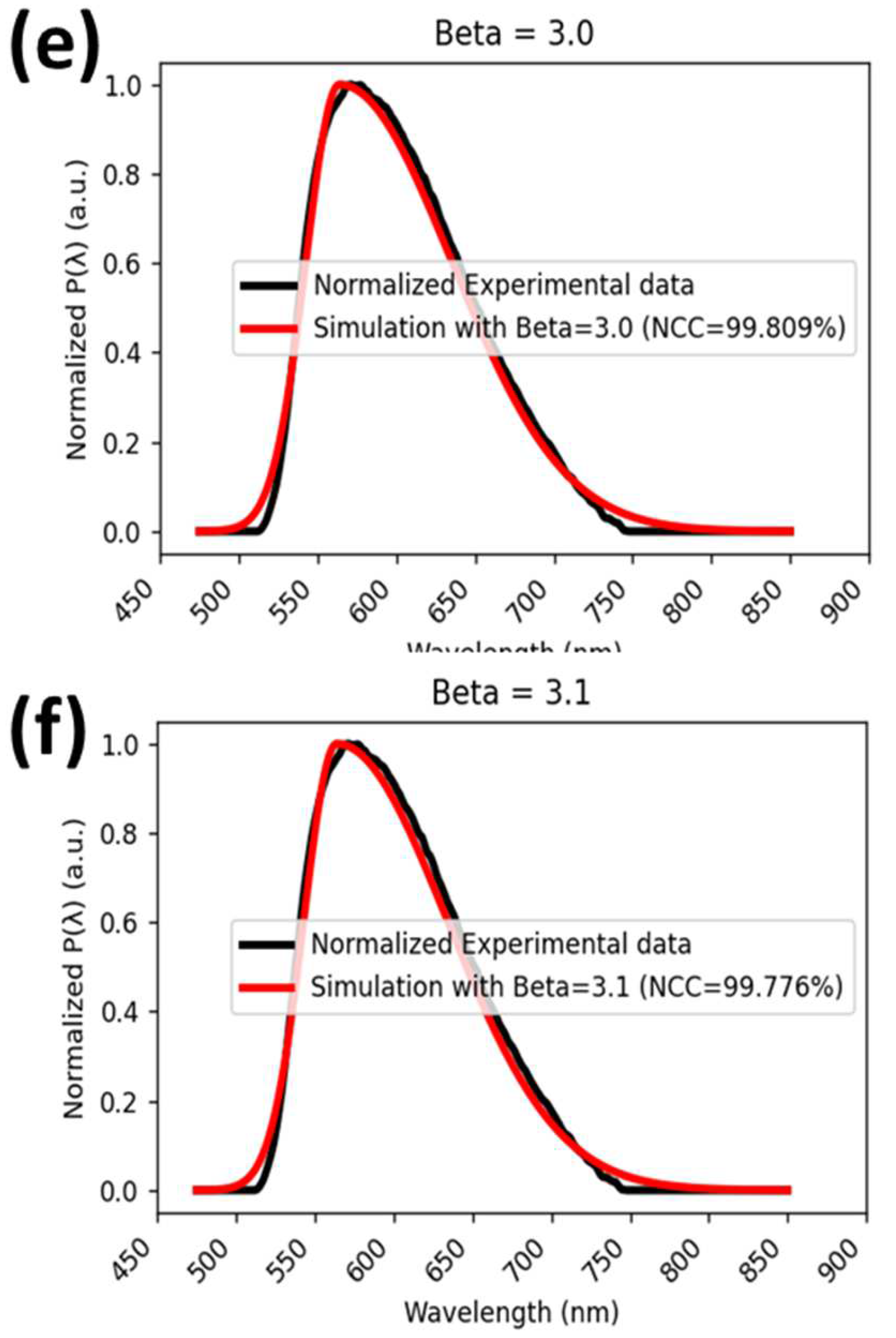
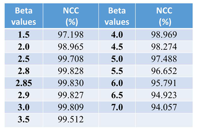
The similarity between simulation and experiment spectrum curves is quantitive evaluated based on the value of NCC (e.g., the value of 100 for NCC means the complete similarity between the simulated and experimental spectrum). The code for optimizing beta value to obtain the highest NCC is shown below, the obtained result is shown in Figure 6 and Table 1.
-
# Calculate NCC value for each beta in beta_step_05 in percentagencc_values = []for beta in beta_step_05:P_lambda_1 = P * np.exp(-beta * ((lambda_experimental_values[lambda_experimental_values <= lambda_mid] - lambda_peak) / 52) ** 2)P_lambda_2 = P * np.exp(-beta * ((lambda_experimental_values[lambda_experimental_values > lambda_mid] - lambda_peak) / 174) ** 2)P_lambda = np.concatenate([P_lambda_1, P_lambda_2])# Compute NCCncc = calculate_ncc(P_lambda, experimental_data)ncc_values.append(ncc)print(f’NCC for Beta = {beta:4.2f} : {ncc:6.3f}%’)# Find the optimal beta valuemax_ncc = max(ncc_values)optimal_beta = beta_step_05[ncc_values.index(max_ncc)]print(f’The maximum NCC value: {max_ncc:.3f}% at Beta = {optimal_beta}’)# Plot the NCC valuesplt.figure(figsize=(8, 5))plt.plot(beta_step_05, ncc_values, ‘o-‘, color=‘red’, linewidth=2, markersize=8, label=‘NCC (%)’)plt.xlabel(‘Value of Beta (β)’, fontsize=12, fontweight=‘bold’)plt.ylabel(‘NCC (%)’, fontsize=12, fontweight=‘bold’)plt.title(‘NCC vs Beta (Step=0.5)’, fontsize=14, fontweight=‘bold’)plt.grid(alpha=0.5)plt.legend()plt.tight_layout()plt.show()
4. Discussions
The method for simulating the emission spectrum of yellow phosphor materials using Python has several applications across various fields in science and engineering. Below are some notable applications, along with examples of how the simulation could be applied in each context:
First, in material science research, emission spectrum modeling is helpful for the characterization and development of new phosphors. Researchers can use the simulation to predict the emission spectra of new phosphor materials. By adjusting the parameters of the Gaussian functions, they can model and visualize how changes in material composition or doping concentration affect the emission spectrum. In developing a new yellow phosphor, the expected emission spectrum is simulated accurately based on theoretical calculations or prior experience with similar materials.
Second, in lighting technology, the emission modeling is applied in the design of LED and lighting Systems. LED manufacturers can apply this method to optimize phosphor blends used in white light LEDs. Simulating the light emitted from yellow phosphors helps engineers select appropriate materials to achieve desired light quality and color rendering (e.g., an engineer designing a white LED might simulate different ratios of yellow phosphors and see how the resulting emission spectrum influences the overall light output and color temperature of the LED).
Third, in display technology, emission modeling can be helpful in the improvement of display systems. Simulation of yellow phosphor emission can aid in the technological development of displays by enhancing color accuracy and brightness in screens (e.g., TVs, monitors). As an application of emission modeling in quantum dot or OLED display technology, understanding how yellow phosphors interact with other colors can improve color balance and intensity. By simulating the emission spectrum, designers can adjust the material properties of quantum dots or phosphors to achieve a better visual experience.
Simulating the emission spectrum of yellow phosphor materials using Python offers several advantages across various disciplines, including research, development, and education. Some of the key advantages are as follows:
First, in term of reducing experimental costs, by simulating the emission spectrum, researchers can explore multiple material compositions and configurations without the need to synthesize every variation. This reduces the cost associated with material procurement and laboratory experiments.
Second, in term of resources, simulations require less physical material, thereby saving on raw materials and minimizing waste.
Third, in term of time efficiency, researchers can quickly modify parameters (like Gaussian parameters) in the simulation to test different hypotheses, enabling faster iteration cycles than traditional experimental methods. It allows for the exploration of a larger number of combinations of material compositions and excitation conditions in a fraction of the time it would take to conduct actual experiments.
Fourth, visualization capabilities are powerful in graphical representation. PYTHON ‘s powerful libraries (like Matplotlib) allow for effective visualization of the emission spectra. Simulations can easily plot multiple emission spectra on the same graph, facilitating comparative analysis of different material configurations or conditions.
Fifth, the customization and flexibility of the emission model are effective. Researchers can build customized models that reflect specific phosphor materials or excitations relevant to their studies, enabling tailored simulations to meet unique project needs. Beyond simple Gaussian functions, more complex models can be integrated as needed, such as Lorentzian peaks, a range of curves, or empirical data fitting.
Sixth, the emission model is important for facilitation of innovation in exploring novel materials. The method encourages the exploration of new yellow phosphors and blends, pushing the boundaries of current materials science and leading to innovations in lighting technology and displays. By simulating the properties of hypothetical materials or configurations, researchers might identify promising candidates for further study, saving time in the exploratory phase of new material development.
5. Conclusions
We proposed and demonstrated a novel solution for modeling the emission of yellow phosphor YAG:Ce3+ by using the PYTHON software. The emission curve is mathematically described by using the Gaussian function. This mathematical model is simulated by programming in PYTHON. The similarities between the simulation and experimental results are compared by the normalized cross-correlation (NCC) algorithm. All NCC values show high values larger than 99.5%. This indicates the high accuracy and trustable degrees of the spectrum model. The proposed model is interesting and meaningful in spectrum modeling for luminescent material with the PYTHON software programming. In addition, the method for simulating the emission spectrum of yellow phosphor materials using Python significantly enhances research and engineering processes. It offers a blend of cost-efficiency, speed, and comprehensive insight while allowing for extensive control and customization. The combination of these advantages positions this method as a powerful tool in materials science, lighting technology, and display.
References
- Schubert, E.-F.; Kim, J.-K. Solid-state light sources getting smart. Science 2005, 308, 1274–1278. [Google Scholar] [CrossRef] [PubMed]
- Narendran, N.; Gu, Y. Life of LED-Based White Light Sources. J. Disp. Technol. 2005, 1, 167–171. [Google Scholar] [CrossRef]
- Schubert, E. Light-Emitting Diodes, 2nd ed.; Cambridge University Press: Cambridge, UK, 2006. [Google Scholar]
- Sun, C.-C.; Nguyen, Q.-K.; Lee, T.-X.; Lin, S.-K.; Wu, C.-S.; Yang, T.-H.; Yu, Y.-W. Active thermal-fuse for stopping blue light leakage of white light-emitting diodes driven by constant current. Sci Rep. 2022, 12, 12433. [Google Scholar] [CrossRef] [PubMed]
- Nguyen, Q.-K.; Glorieux, B.; Sebe, G.; Yang, T.-H.; Yu, Y.-W.; Sun, C.-C. Passive anti-leakage of blue light for phosphor-converted white LEDs with crystal nanocellulose materials. Sci Rep. 2023, 13, 13039. [Google Scholar] [CrossRef]
- Nguyen, H.-T.-A.N.Q.-K. An Investigation on the Optical Characteristic of the Phosphor-Converted White Light-Emitting DiodesBased Flash Light Source of Commercial Smartphone. J. Mater. Eng. 2023, 3, 148–156. [Google Scholar] [CrossRef]
- Xie, R.-J.; Li, Y.Q.; Hirosaki, N.; Yamamoto, H. Nitride Phosphors and Solid-State Lighting, 1st ed.; CRC Press, 2011. [Google Scholar]
- Nguyen, H.-T.-A.; Huynh, V.-T.; Nguyen, Q.-C.; Nguyen, Q.-K. High-accuracy emission modeling of yellow phosphor YAG: Ce validated by normalized cross-correlation. Photonics Lett. Pol. 2024, 16, 31–33. [Google Scholar]
- Yang, T.-H.; Huang, H.-Y.; Sun, C.-C.; et al. Noncontact and instant detection of phosphor temperature in phosphor-converted white LEDs. Sci. Rep. 2018, 8, 296. [Google Scholar] [CrossRef]
- de Bonfils, J.; Panczer, G.; de Ligny, D.; Peuget, S.; Delaye, J.-M.; Chaussedent, S.; Monteil, A.; Champagnon, B. Simulation of Eu3+ luminescence spectra of borosilicate glasses by molecular dynamics calculations. Opt. Mater. 2008, 30, 1689–1693. [Google Scholar] [CrossRef]
- Koryukina, E.V.; Koryukin, V.I. Simulation of Emission Spectra of Light Sources Based on an Inductive Discharge. Russ. Phys. J. 2017, 59, 1996–2003. [Google Scholar] [CrossRef]
- Avtaeva, S. Modeling of the Sulfur Emission in the Asymmetric Pulse Dielectric Barrier Discharge. Plasma Chem Plasma Process 2023, 43, 867–877. [Google Scholar] [CrossRef]
- Xie, A.G.; Liu, Y.F.; Dong, H.J. Secondary electron emission model for photo-emission from metals in the vacuum ultraviolet. Nucl. Sci. Tech. 2022, 33, 103. [Google Scholar] [CrossRef]
- Sivadas, M.S.S.; John, L.M.; Anoop, K.K. Simulation of Optical Emission Spectra of Cu-Sn-Zn Alloy Plasmas for Laser-Induced Breakdown Spectroscopy Applications. 2022 IOP Conf. Ser. Mater. Sci. Eng. 2022, 1221, 012027. [Google Scholar] [CrossRef]
- Vu, T.-H.-T.; Nguyen, Q.-K. Precision optical model of asymmetry emission band of red light emitting diodes and its application in improving the color rendering index of white LEDs. Results Opt. 2025, 21, 100825. [Google Scholar] [CrossRef]
- Nguyen, Q.-K. Emission spectrum modeling of white LEDs light source with using Gaussian function. Photonics Lett. Pol. 2023, 15, 54–56. [Google Scholar] [CrossRef]
- Chien, W.-T.; Sun, C.-C.; Moreno, I. Precise optical model of multi-chip white LEDs. Optics Express 2007, 12, 7572–7577. [Google Scholar] [CrossRef] [PubMed]
- Sun, C.-C.; Chen, C.-Y.; He, H.-Y.; Chen, C.-C.; Chien, W.-T.; Lee, T.-X.; Yang, T.-H. Precise optical modeling for silicate-based white LEDs. Optics Express 2008, 16, 20060–20066. [Google Scholar] [CrossRef]
- Vo, T.-M.-L.; Tran, T.-N.; Nguyen, T.-K.; Nguyen, T.-H.; Pham, T.-Y.-N.; Huynh, T.-B.; Pham, L.-M.-K.T.D.-K.; Nguyen, Q.-C.; Nguyen, Q.-K. Development of an efficient optical model for LEDs-based white light spectrum design applications. J. Innov. Bus. Ind. 2024, 2, 185–192. [Google Scholar] [CrossRef]
- Nguyen, H.-T.-A.; Nguyen, Q.-K. Study of high-accuracy optical model of green phosphor pumped by ultraviolet laser. Results Opt. 2025, 18, 100780. [Google Scholar] [CrossRef]
- Smet, K.A.G. Tutorial: The LuxPy Python Toolbox for Lighting and Color Science. LEUKOS 2019, 16, 179–201. [Google Scholar] [CrossRef]
- Sun, C.-C.; Lee, T.-X.; Ma, S.-H.; Lee, Y.-L.; Huang, S.-M. Precise optical modeling for LED lighting verified by cross correlation in the midfield region. Opt. Lett. 2006, 31, 2193–2195. [Google Scholar] [CrossRef]
- Nguyen, H.-T.-A.; Huynh, V.-T.; Nguyen, Q.-C.; Nguyen, Q.-K. High-accuracy emission modeling of yellow phosphor YAG: Ce validated by normalized cross-correlation. Photonics Lett. Pol. 2024, 16, 31–33. [Google Scholar]
Figure 1.
Illustrates the principle of white light generation of yellow phosphor under excitation of blue LED sources.
Figure 1.
Illustrates the principle of white light generation of yellow phosphor under excitation of blue LED sources.
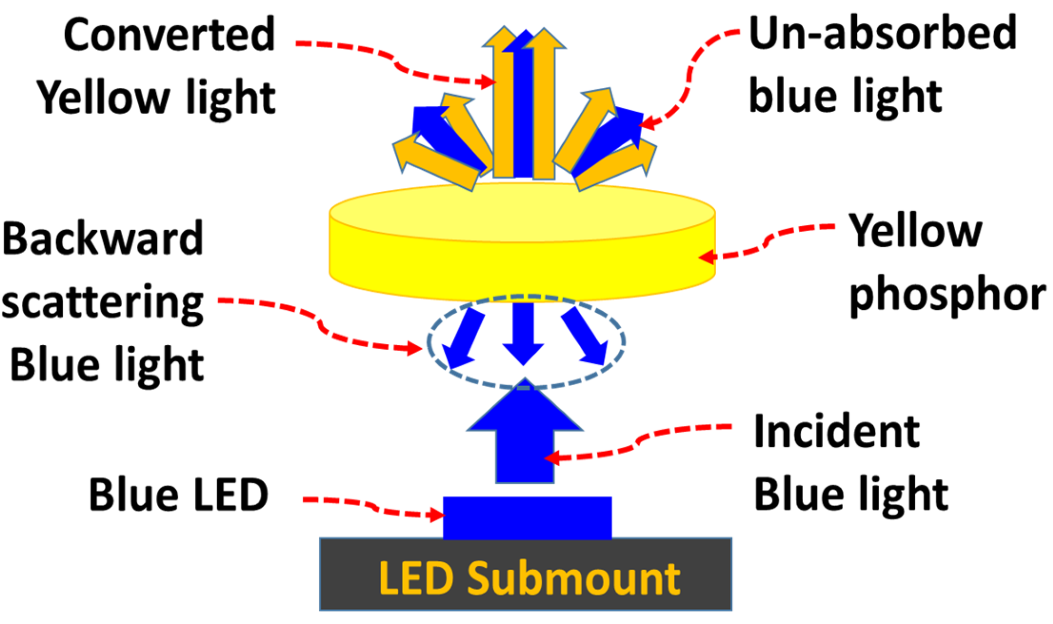
Figure 2.
The electronics transition during long wavelength conversion process of yellow phosphor.
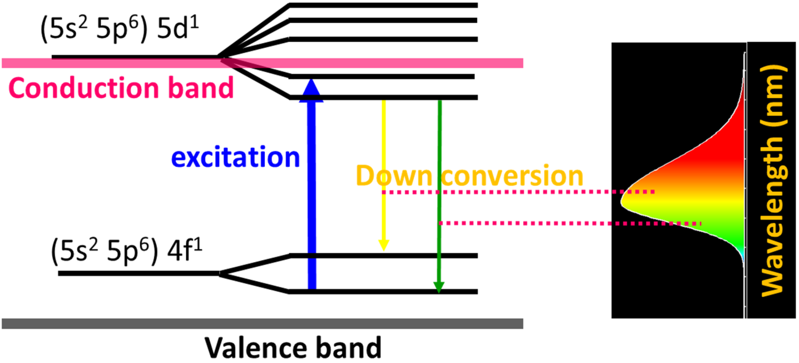
Figure 3.
Illustration of analysis of the curve of the yellow emission spectrum to simplify the simulation process.
Figure 3.
Illustration of analysis of the curve of the yellow emission spectrum to simplify the simulation process.
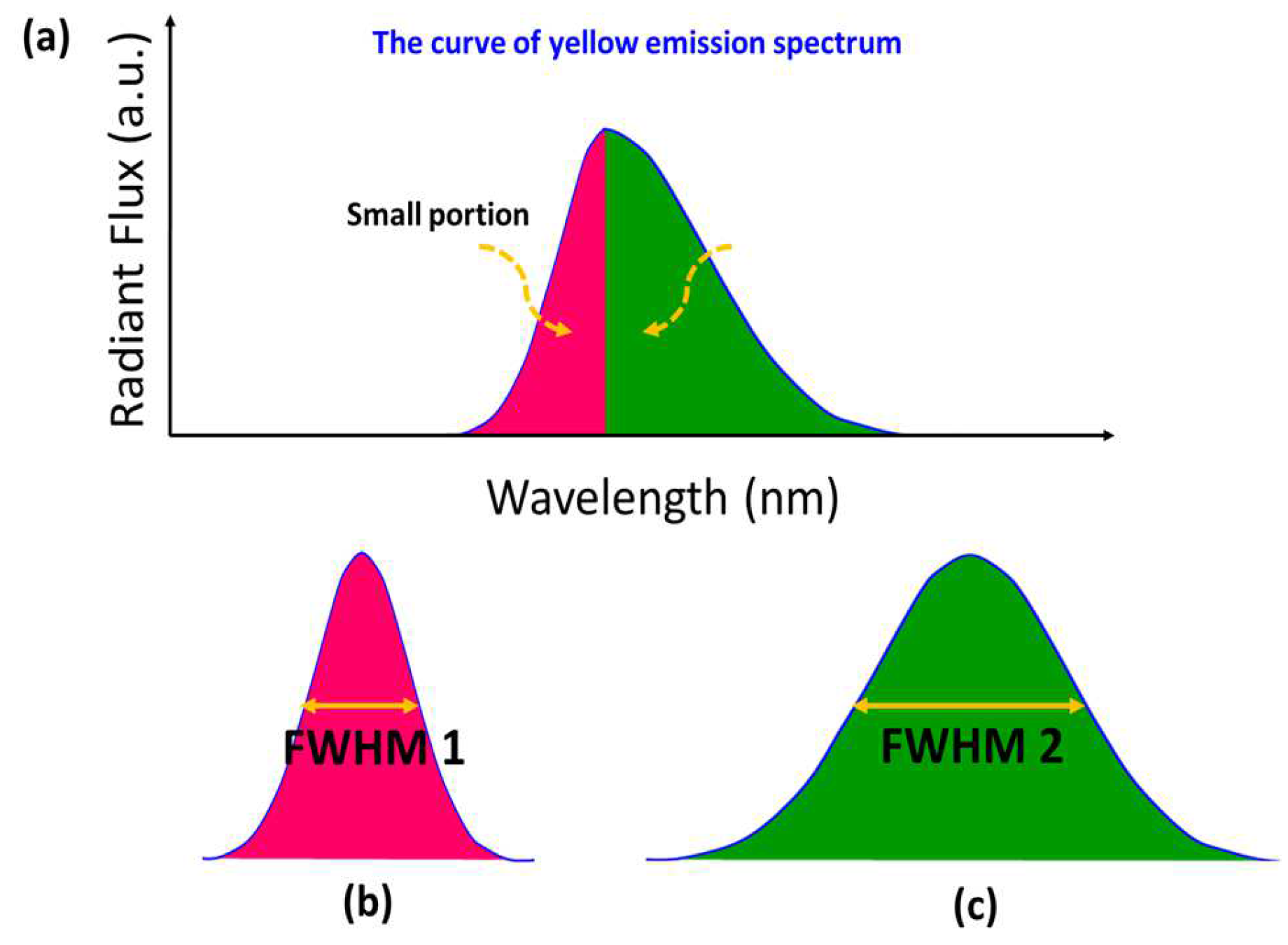
Figure 4.
Simulation spectrum of yellow emission using PYTHON.
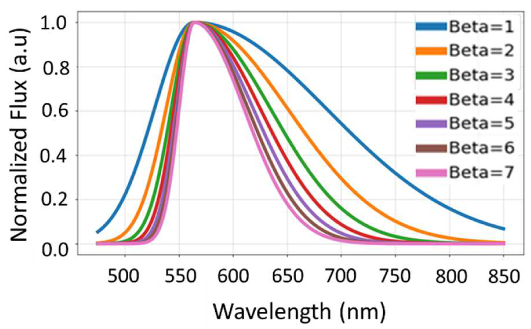
Figure 6.
Optimize beta value to obtaine the highest NCC.
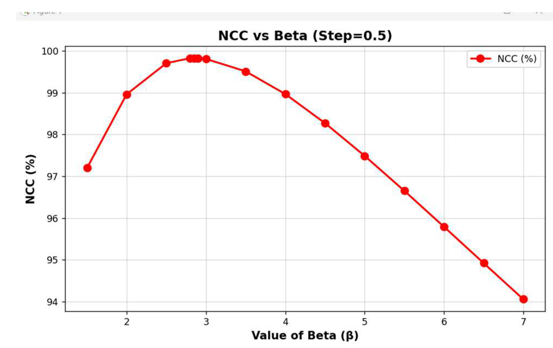

Table 1.
Changing of NCC versus Beta values.
 |
Disclaimer/Publisher’s Note: The statements, opinions and data contained in all publications are solely those of the individual author(s) and contributor(s) and not of MDPI and/or the editor(s). MDPI and/or the editor(s) disclaim responsibility for any injury to people or property resulting from any ideas, methods, instructions or products referred to in the content. |
© 2025 by the authors. Licensee MDPI, Basel, Switzerland. This article is an open access article distributed under the terms and conditions of the Creative Commons Attribution (CC BY) license (https://creativecommons.org/licenses/by/4.0/).
Copyright: This open access article is published under a Creative Commons CC BY 4.0 license, which permit the free download, distribution, and reuse, provided that the author and preprint are cited in any reuse.


