Submitted:
06 May 2025
Posted:
09 May 2025
You are already at the latest version
Abstract
Ignition delay time (IDT) is a fundamental parameter in fuel combustion, with accurate prediction across temperature ranges remaining a significant research challenge. RP-3, a widely used aviation kerosene, plays a key role in refining chemical kinetics and optimizing aeroengine combustion design. This study presents a BP neural network prediction framework, enhanced through random selection and gradient descent optimization, to achieve high-precision IDT prediction under various conditions.The proposed model features five inputs and one output, with hidden layer structure optimized using a random selection strategy to improve generalization and robustness. Among five gradient descent algorithms evaluated, the conjugate gradient method paired with a [21, 17, 19] three-hidden-layer architecture achieved the best performance (R² = 0.99705, MAPE = 1.2%, MAE = 0.0287, RMSE = 0.0359). The model maintained high accuracy across equivalence ratios (φ = 1.0–2.0) and pressures (10–20 bar).Sensitivity and importance analysis revealed that temperature and diluent mole fraction significantly influence IDT, especially in the lowand high-temperature and NTC regions. Overall, the proposed method demonstrates strong generalization, robustness, and application potential, offering a data-driven tool for modeling combustion characteristics of complex aviation fuels.
Keywords:
Ignition delay time
; RP-3 aviation kerosene
; BP neural network
; Gradient descent algorithm
; Sensitivity analysis
; Importance assessment
1. Introduction
Ignition Delay Time (IDT) serves as a critical parameter for evaluating the autoignition characteristics and ignition flammability of fuels. As an essential indicator of fuel autoignition performance, it plays a pivotal role in assessing combustion behavior in aeroengines and developing high-fidelity combustion models. Currently, the most widely adopted IDT measurement techniques include Shock Tube [1-4], Constant Volume Combustion Bomb (CVCB) [5], and Rapid Compression Machine (RCM) [6-9]. Moreover, with advancements in optical diagnostic technologies, methods such as Laser-Induced Fluorescence (LIF) and absorption spectroscopy have been integrated into IDT research [10], substantially enhancing measurement accuracy and resolution. These techniques provide robust data support for constructing high-precision ignition prediction models. However, due to the complex coupling effects of variables such as temperature, pressure, equivalence ratio, and fuel molecular structure on IDT, its prediction problem exhibits highly nonlinear and multi-dimensional characteristics. Traditional approaches based on detailed mechanism models (e.g., CHEMKIN) [11-19] offer reasonable accuracy but involve significant computational demands during modeling and solving processes. Additionally, these methods are sensitive to initial conditions and are unsuitable for real-time engineering predictions.
Neural networks, particularly the "Backpropagation Neural Network (BP Neural Network)" , a canonical feedforward neural network, have demonstrated the ability to effectively approximate any nonlinear function structure and have been widely applied in recent years for the rapid prediction of ignition delay time (IDT). This methodology leverages experimental or simulation data to establish nonlinear mappings between inputs (e.g., initial temperature, pressure, equivalence ratio, oxygen concentration, etc.) and outputs (IDT) by training the weights. Wu et al. [20] utilized a three-layer BP neural network model in their study, employing temperature, pressure, and equivalence ratio as input variables to predict the IDT of various fuels (including methane, n-heptane, etc.), achieving a determination coefficient exceeding 0.98. Liu and Chen [21] further developed a deep feedforward neural network (DNN) for the alternative aviation fuel system (synthetic oil and bio-jet fuel), attaining superior mean absolute error (MAE) performance across a broader temperature range, with the error maintained within 3 ms. Wang et al. [22] conducted a comparative analysis of Jet-A alternative fuel IDT predictions using three methods: BP neural network, Random Forest (RF), and Support Vector Machine (SVM). Their findings indicated that the BP neural network outperformed the other two algorithms in medium and high-temperature regions, showcasing fast training speed and strong generalization ability. Beyond conventional BP networks, some studies have explored more complex architectures to enhance model performance.Zhang and Lin [23] introduced a method leveraging Convolutional Neural Networks (CNNs) to extract local features of temperature-pressure-component variables, thereby predicting the Ignition Delay Time (IDT) under complex operating conditions. Patel and Saxena [24] employed Long Short-Term Memory Networks (LSTMs) to process time-evolving temperature field and concentration gradient data, enhancing dynamic prediction capabilities in modeling. Moreover, neural network-based IDT modeling has been extended to multi-component fuel systems, including complex aviation kerosenes such as RP-3 and Jet-A. Wang et al. [25] utilized experimental data to train a neural network for predicting the IDT of RP-3 kerosene under shock tube conditions and validated the model's universality across multiple equivalence ratios and pressure ranges. Their results exhibited a prediction error of less than 5%, significantly outperforming polynomial regression models. Ji et al. [26] demonstrated that optimization based on Stochastic Gradient Descent (SGD) enables the neural network model to effectively represent Hybrid Chemistry pyrolysis while optimizing hundreds of related weights within the network. Additionally, to improve the interpretability and generalizability of the models, some studies have integrated techniques such as parameter normalization, feature importance analysis (e.g., SHAP values), cross-validation, and transfer learning strategies, ensuring high accuracy even in scenarios with small sample sizes or predictions for new fuels [27, 28].
To sum up, the application of neural networks in predicting ignition delay time has evolved from simple single-fuel BP modeling to a sophisticated multi-fuel, multi-structure, and multi-input variable modeling system. This advancement has become an essential technical approach for the rapid evaluation of aviation fuels and the optimization of engineering models. However, there is still a lack of systematic comparison regarding the effects of different gradient descent algorithms on the prediction accuracy of RP-3 ignition delay time. Based on this consideration, this paper proposes a BP neural network model that employs various gradient descent algorithms to fit and predict the RP-3 ignition delay time under diverse operating conditions via a random search method.
2. Materials and Methods
2.1. Data collection and preparation
The dataset of RP-3 ignition delay time utilized in this study is sourced from the literature [29-34], comprising a total of 700 data points. The temperature range of the dataset spans from 640 to 1600 K, the ambient pressure varies between 0.5 and 20 bar, and the equivalence ratio φ ranges from 0.2 to 2.0. These parameters effectively capture the reaction delay characteristics of RP-3 under diverse combustion conditions. Specifically, 560 data points (80%) are allocated to the training set, 70 data points (10%) to the validation set, and another 70 data points (10%) to the test set. Additionally, the logarithm of the RP-3 ignition delay time dataset is computed to mitigate the order-of-magnitude differences, linearize the complex relationships, and enhance both the stability and predictive accuracy of the model during training.
2.2. BP neural network algorithm
BP neural network (Back Propagation Neural Network) is a training algorithm for multi-layer feedforward neural networks based on the error backpropagation mechanism (Back Propagation Algorithm). It serves as a critical tool in machine learning for tasks such as classification and regression. The network computes the output result via forward propagation and subsequently propagates the output error layer by layer through backward propagation. Simultaneously, it employs an optimization algorithm to iteratively adjust the weights and biases of the network, thereby minimizing the prediction error and achieving objectives such as classification, regression, and function approximation for given input data.
Based on Matlab, a BP neural network consisting of an input layer, a hidden layer, and an output layer was constructed. The input layer comprised five neurons corresponding to the mixture gas pressure, ignition temperature, oxidant mole fraction, fuel mole fraction, and diluent mole fraction. The output layer consisted of a single neuron representing the ignition delay time. The initial learning rate for the BP neural network was set to 0.01, with a minimum error target of 0.005. The structural diagram of the neural network is presented in Figure 1.
In the actual modeling process, adopting a fixed network structure configuration (e.g., the number of hidden layers, the number of neurons, and the activation function) is prone to limiting the model's generalization ability or causing it to become trapped in local optima. To further enhance the robustness and prediction accuracy of the model, this paper proposes a random selection strategy for multiple rounds of combination and training of key hyperparameters in the BP neural network. This strategy primarily focuses on the following three aspects:
(1) Random sampling of the number of neurons in the hidden layer: The number of neurons in each layer is randomly sampled within five predefined interval ranges, namely [5-15,15-25,25-35,35-45], and [45-55]. This approach effectively avoids potential underfitting or overfitting issues that may arise from a fixed network structure.
(2) Random combination of activation functions: The candidate activation functions consist of tansig (hyperbolic tangent function), logsig (logarithmic sigmoid function), and purelin (linear function). During each training iteration, the activation functions for the hidden layer and output layer are randomly paired, enabling the model to adaptively adjust its nonlinear feature representation capabilities. In configurations with multiple hidden layers, this strategy effectively mitigates the limitations imposed by a single activation function on nonlinear learning, thereby enhancing the overall prediction performance.
(3) Random perturbation of initialization weights and biases: Network parameters are initialized using different random seeds, and multiple training runs are performed for each network structure. Models achieving an R² greater than 0.95 and MAE, MAPE, and RMSE values below 0.1, 4%, and 0.1, respectively, are considered to exhibit superior generalization performance. Ultimately, based on the results of random sampling during training, the model configuration demonstrating the best generalization performance is selected as the candidate model according to the R², MAE, MAPE, and RMSE metrics.
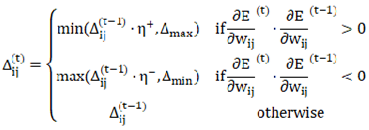
2.3. Gradient descent algorithm
Gradient Descent is a classical and extensively utilized optimization algorithm, primarily employed for minimizing the objective function. It plays a pivotal role, particularly in the training of machine learning and deep learning models. The fundamental concept involves iteratively updating model parameters to progressively approach the optimal solution along the negative gradient direction of the objective function. Below are the types of gradient descent algorithms utilized in this study.
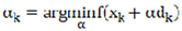
- 1.
- Standard Gradient Descent (SGD)
Standard gradient descent serves as the foundational optimization algorithm in deep learning models. Its primary concept involves leveraging the gradient information of the loss function with respect to the parameters to update the model parameters in the direction opposite to the gradient. The formula for each iterative update is as follows:
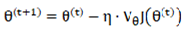
Where denotes the model parameters, represents the learning rate, and  stands for the gradient of the loss function with respect to the parameters for the current batch of samples.
stands for the gradient of the loss function with respect to the parameters for the current batch of samples.- 2.
- Momentum Gradient Descent (MGD)
To address the issue of slow convergence of Stochastic Gradient Descent (SGD) in regions with high curvature or non-convexity, the momentum term (Momentum) is incorporated. This method is inspired by the inertial concept in physics, leveraging both current and historical gradient information to mitigate oscillations and enhance convergence speed. The computation is defined by Equations (2) and (3).
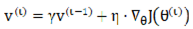
Whererepresents the accumulated momentum, and denotes the momentum
factor, which is typically set to 0.9.
denotes the momentum
factor, which is typically set to 0.9.
denotes the momentum
factor, which is typically set to 0.9.- 3.
- Adaptive Gradient Algorithm (AGA)
The adaptive gradient algorithm proposes to design a learning rate for each parameter individually and adjust the update amplitude of each step based on the historical accumulation of squared gradients. This mechanism provides the model with an advantage when handling sparse data or when features exhibit varying levels of importance. The calculation formulas are presented in Equations (4) and (5).
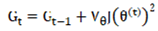
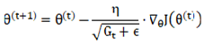
Wheredenotes the accumulation of squared historical gradients for each parameter; is a very small constant introduced to avoid division by zero;  represents the initial learning rate, and
  indicates
the current gradient.
indicates
the current gradient.
represents the initial learning rate, and indicates
the current gradient.- 4.
- Resilient Backpropagation (RPROP)
The traditional backpropagation (BP) algorithm utilizes the gradient descent method to update the neural network weights based on the derivative of the error function. However, in practical applications, the BP algorithm is prone to several challenges: vanishing gradients (gradients that become excessively small), which can result in slow or stagnant learning; exploding gradients (gradients that become excessively large), leading to divergence; and difficulties in adjusting the learning rate, causing oscillations when it is too high and slow convergence when it is too low. To address these limitations, the resilient backpropagation algorithm determines the direction of weight updates based on the "sign" of the partial derivative of the error function with respect to the weights, disregarding its specific magnitude. Each weight has its own independent step size for updates, which is adaptively adjusted according to the trend of changes in the sign of the derivative. The calculation method is provided by Equations (6) and (7).
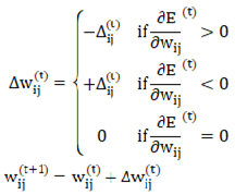
Where the derivative of the error function with respect to the weight is denoted as  the update step size as , and the weight update as ·
  represents the initial step size,
  represents the maximum step size, and
  represents the minimum step size. Additionally denotes the increase factor, while represents the decrease factor.
the update step size as , and the weight update as · represents the initial step size, represents the maximum step size, and represents the minimum step size. Additionally denotes the increase factor, while represents the decrease factor.- 5.
- Conjugate Gradient Descent (CGD)
The conjugate gradient method was initially developed for solving large-scale linear systems and has been adapted for use in neural networks as an approximate second-order optimization algorithm. Unlike traditional first-order methods, it avoids the explicit storage of the full Hessian matrix. Compared to stochastic gradient descent (SGD), the conjugate gradient method demonstrates a faster convergence rate. Its fundamental update rules are presented in Equations (8), (9), and (10).
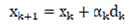
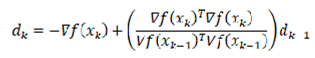
Where represents the objective function, denotes the iteration variable, signifies the gradient, corresponds to the conjugate direction, and indicates the step size.
2.4. Evaluation of models
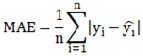
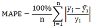
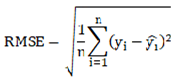
After training, the BP neural network generally requires evaluation of its prediction performance and generalization ability using a set of metrics. To comprehensively assess the performance of the delayed ignition time prediction model, this paper selected several widely used evaluation metrics in regression analysis. These include Mean Absolute Error (MAE), Mean Absolute Percentage Error (MAPE), Root Mean Squared Error (RMSE), and the coefficient of determination (R-squared, R²). These metrics evaluate the prediction accuracy, stability, and degree of fit to actual values from different perspectives, providing a quantitative basis for model tuning and practical engineering applications. Among these, one of the most fundamental regression error measures is the Mean Absolute Error (MAE), which represents the average of the absolute differences between predicted and actual values. Its calculation method is provided in equation (11), where denotes the actual value of the ith sample, is its corresponding predicted value, and is the total number of samples. MAE assigns equal weight to each sample, is straightforward to compute, and is less sensitive to outliers. A model with lower overall error will exhibit a smaller MAE value. In contrast, the Mean Absolute Percentage Error (MAPE) further standardizes the error by expressing it as a percentage relative to the true value, as calculated in equation (12).
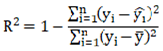
Furthermore, the coefficient of determination (R²) serves as a critical metric for evaluating how well the model fits the data. It quantifies the proportion of variance in the dependent variable that is predictable from the independent variable(s). A value of R² closer to 1 indicates a better fit of the model, while a negative value suggests that the model performs worse than a simple mean prediction. The calculation of R² is presented in Formula (13).
Wherein,  s the average of the true values.
s the average of the true values.Nevertheless, during the actual construction and training of the model, it was found that the aforementioned three evaluation indices fail to provide a satisfactory assessment of the fitting effect for certain outliers within the model. Therefore, the root mean square error (RMSE) is introduced as an additional evaluation metric to enhance the comprehensive evaluation of the model's fitting performance. RMSE builds upon the mean absolute error (MAE) by incorporating a squared term and subsequently taking the square root, thereby more prominently emphasizing the impact of larger prediction errors. Given its heightened sensitivity to large errors, RMSE is particularly suitable for evaluating the fitting performance in high-precision model predictions where significant outliers or occasional extreme events (e.g., exceptionally high delay times) may occur in the system. The calculation method for RMSE is provided in Formula (14).
This research, by leveraging the multi-dimensional performance evaluation indicators outlined above, can systematically assess the strengths and weaknesses of the model in terms of error magnitude, error trend, degree of fitting, and relative performance. This provides a robust and scientific foundation for subsequent model optimization and practical applications.
3. Results
3.1. Determination of the Optimal Hidden Layer
In a BP neural network, the design of the hidden layer structure is one of the critical factors influencing the model's performance. The appropriate configuration of layers and neurons not only affects the model's approximation and learning capabilities but also determines its training efficiency and generalization ability. To construct an optimal network structure for predicting the ignition delay time of RP-3 aviation kerosene, this paper proposes two-hidden-layer and three-hidden-layer structures based on empirical formulas and practical fitting results. Furthermore, it systematically adjusts the number of neurons in the hidden layers to conduct an in-depth investigation into the hidden layer configuration for predicting the ignition delay time of RP-3.
In previous BP neural networks, the selection of the number of hidden layer nodes typically uses the empirical formula:

Where is the number of input layer nodes, is the number of output layer nodes, and C is an empirical constant, usually ranging from 1 to 10. However, the number of hidden layer nodes selected based on the empirical formula is solely determined by the number of input and output layer nodes. In practice, the required number of nodes often exceeds the value suggested by the empirical formula. Therefore, for the multi-input variable ignition delay data analyzed in this study, the range of hidden layer nodes derived from the empirical formula is [5–15]. To explore a broader range, we extend the number of hidden layer nodes to [15–55]. Among the 50 possible node numbers within this extended range, the optimal hidden layer configuration is defined as the one achieving the maximum R² value on the test set. By randomly selecting the specified number of hidden layer nodes within the five subranges of [5–15,15–25,25–35,35–45], and [45–55], two-hidden-layer and three-hidden-layer networks are constructed. The performance of these models within each subrange is evaluated using R², MAE, and MAPE metrics.
For the double and triple hidden-layer models, 30 repeated calculations were performed within the range of 5 to 20 neurons using the standard gradient descent algorithm. The results are presented in Figure 2 and Figure 3. All models shared the same initial learning rate and activation function. Figure 2 and Figure 3 correspond to the performance comparison of the double and triple hidden-layer structures, respectively, within the range of 5 to 20 neurons. These figures clearly illustrate the performance differences of neural network structures with varying numbers of hidden layers under different neuron configurations.

Table 1.
Training results across different hidden-layer configurations.
| Hidden-layer Structure | Range of the hidden layer | R2 | MAPE(%) | MAE |
|---|---|---|---|---|
| two-hidden-layer structure | [5-15] | 0.91099 | 5.23362 | 0.11951 |
| [15-25] | 0.93781 | 3.57593 | 0.081 | |
| [25-35] | 0.90006 | 4.77065 | 0.1167 | |
| [35-45] | 0.94042 | 3.62867 | 0.08418 | |
| [45-55] | 0.92087 | 3.88182 | 0.08478 | |
| three-hidden-layer structure | [5-15] | 0.90349 | 4.50252 | 0.10757 |
| [15-25] | 0.94449 | 2.87703 | 0.0679 | |
| [25-35] | 0.95831 | 2.77153 | 0.07051 | |
| [35-45] | 0.9418 | 3.24754 | 0.08054 | |
| [45-55] | 0.9339 | 3.14394 | 0.08222 |
It can be observed from Figure 1, Figure 2, and Tab.1 that the overall fitting performance of the three-hidden-layer structure is superior to that of the two-hidden-layer structure. Across the entire neuron range, the average coefficient of determination R² for the three-hidden-layer structure is consistently higher than that of the two-hidden-layer structure, particularly in the intervals [15-25,25-35,35-45], and [45-55], where it exceeds 0.93. Additionally, both the MAPE and MAE metrics are relatively low, with minimum values of 2.7715% and 0.0679, respectively, indicating that the three-hidden-layer structure offers greater advantages in terms of fitting and prediction accuracy. Although the two-hidden-layer model achieves a relatively high R²(approximately 0.94) in certain intervals (e.g., [35-45]), its error volatility across the hidden layer range is larger, and its stability is inferior to that of the three-hidden-layer structure.
When the number of hidden layer neurons is excessively small (e.g., [5-15]), the model experiences underfitting, leading to a low R² value and substantial errors. This confirms that for ignition delay data with multiple input variables, the number of hidden layer nodes determined by empirical formulas does not yield optimal fitting results. When the number of neurons is moderate (e.g., [15-35]), the model can effectively capture data characteristics while maintaining error control. In cases where the number of neurons is excessive (e.g., [45-55]), although training accuracy improves marginally, test errors slightly increase, indicating the onset of overfitting. Multiple training instances reveal that the error variation trends of the three-hidden-layer model on both the training and validation sets are consistent, demonstrating excellent generalization ability. Moreover, from the perspective of network stability, the performance fluctuations of the three-hidden-layer structure under different batch divisions are minimal, suggesting that this architecture is more robust.
In conclusion, by comprehensively evaluating the model's fitting capability, error performance, training stability, and complexity balance, the three-hidden-layer structure, with the number of neurons in each layer ranging from 15 to 35, is ultimately determined as the optimal structural configuration for this study.
3.2. Neural networks founded on diverse gradient descent algorithms
To further enhance the prediction performance of the BP neural network for the ignition delay time of RP-3 aviation kerosene, this article introduces and compares five typical gradient optimization algorithms: Standard Gradient Descent, Momentum Gradient Descent, Adaptive Gradient Algorithm, Resilient Backpropagation, and Conjugate Gradient Descent. By incorporating the interval variations of the number of neurons in the hidden layer, specifically [5−15,15−25,25−35,35−45], and [45−55], multiple experiments were conducted. The prediction performance of each algorithm under different network configurations was evaluated using three metrics: R², Mean Absolute Error (MAE), and Mean Absolute Percentage Error (MAPE). The results are presented in Figure 4,Figure 5 and Figure 6.
It can be observed from the above pictures that the conjugate gradient descent method demonstrates a markedly superior fitting capability across all neuron intervals. The R² value remains consistently above 0.98, reaching a peak of 0.99705 in the [25-35] interval, which is nearly indistinguishable from 1. In contrast, the R² value of the standard gradient descent method exhibits significant fluctuations, with the maximum deviation approaching 0.09, indicating its limited ability to fit complex nonlinear relationships. The elastic backpropagation algorithm and the adaptive gradient algorithm also perform well in most intervals; however, the R² value of the adaptive gradient algorithm slightly decreases in intervals with extremely small or large numbers of neurons. Furthermore, based on the MAE distribution results, the conjugate gradient descent method achieves the lowest error of 0.035 in the [15-25] interval, significantly outperforming other algorithms in terms of prediction accuracy and stability. The elastic backpropagation method shows comparable performance in the middle interval [15-25]. Conversely, the MAE of the standard gradient descent method exceeds 0.07 in all intervals, with noticeable fluctuations. Additionally, the conjugate gradient descent method exhibits the lowest MAPE in the [15-25] interval, approximately 1.2%, and maintains a MAPE below 2.5% across all intervals. By comparison, the MAPE of the standard gradient descent method surpasses 4% in some intervals, demonstrating its inferior performance. The trend of MAPE further corroborates the aforementioned conclusions. Overall, the conjugate gradient descent method clearly outperforms other optimization algorithms in terms of fitting accuracy and error control.
In the comparative experiment between the double-hidden-layer and triple-hidden-layer structures presented in Section 3.1, the triple-hidden-layer structure exhibited superior R² scores, smaller MAE, and lower MAPE values across most configurations. This indicates its stronger generalization capability and enhanced fitting performance. Furthermore, in conjunction with the results depicted in Figure , it is evident that the triple-hidden-layer structure performs exceptionally well within the [15-35] neuron range. Specifically, the conjugate gradient descent method achieves optimal overall performance within this range. To ascertain the ideal number of neurons for the model, this study identified the best-performing models corresponding to each gradient descent algorithm within the [15-35] neuron range during training and visualized these findings in Figure 7 for direct comparison. The radar chart reveals that the model with [21 17 19] neurons under the conjugate gradient descent algorithm excels across all five evaluation metrics, showcasing the smallest error contour. Consequently, the model featuring a triple-hidden-layer neuron distribution of [21 17 19], utilizing the conjugate gradient descent method and a random activation function strategy, was ultimately selected as the optimal network structure configuration for this study.
3.3. Determination of the Optimal Hidden Layer
3.3.1. The predictive performance of the model
It can be observed from Figure 8 that under the working condition of φ= 1.0, the overall trend of the prediction points closely matches the actual points across various pressure conditions. Specifically, under medium and low pressure conditions, the prediction points at 10 bar and 15 bar almost entirely overlap with the actual points, indicating the model's high prediction accuracy and consistency in lower pressure ranges. However, under the high-pressure condition of 20 bar, some prediction points show slight deviations from the actual points, although the deviation is minimal and the overall trend remains consistent. This underscores the model's reliability for IDT prediction under high-pressure conditions and further validates its excellent fitting capability across a wide range of pressures.
Further, in the image with φ= 1.5 (Figure 9), the correlation between the predicted points and the actual points is significantly enhanced across all pressure conditions. The ignition delay time variation under different pressures is precisely captured by the predicted points, showing a stable distribution with minimal deviations. Within the pressure range of 10–20 bar, the predicted points exhibit excellent agreement with the experimental data. Notably, at pressures of 10 bar and 20 bar, the predicted points almost perfectly overlap with the actual points, indicating that the model achieves high fitting accuracy and demonstrates robust generalization performance in the medium equivalence ratio and high-pressure regime.
The reaction pathway of the fuel in a fuel-rich environment is highly complex. For the operating condition with φ= 2.0, the performance at various pressure points shows nuanced differences, as depicted in Figure 10. At 20 bar, the predicted values are closely aligned with the actual values. However, in the lower-pressure range, the predicted values exhibit a certain degree of systematic deviation, where they tend to be slightly higher or lower than the actual values. Despite this, the predicted values generally follow the variation trend of the actual values without significant deviation in the overall trend.
In summary, as illustrated in Figure 8, Figure 9, and Figure 10, the BP neural network model demonstrates excellent prediction consistency under most pressure conditions, particularly exhibiting robust performance in medium and low-pressure environments. At a few specific points under certain operating conditions, the prediction error marginally increases, indicating that there is still potential for improving the model's accuracy. The model prediction outcomes from this study provide a solid foundation for further refining model training and optimizing sample distribution.
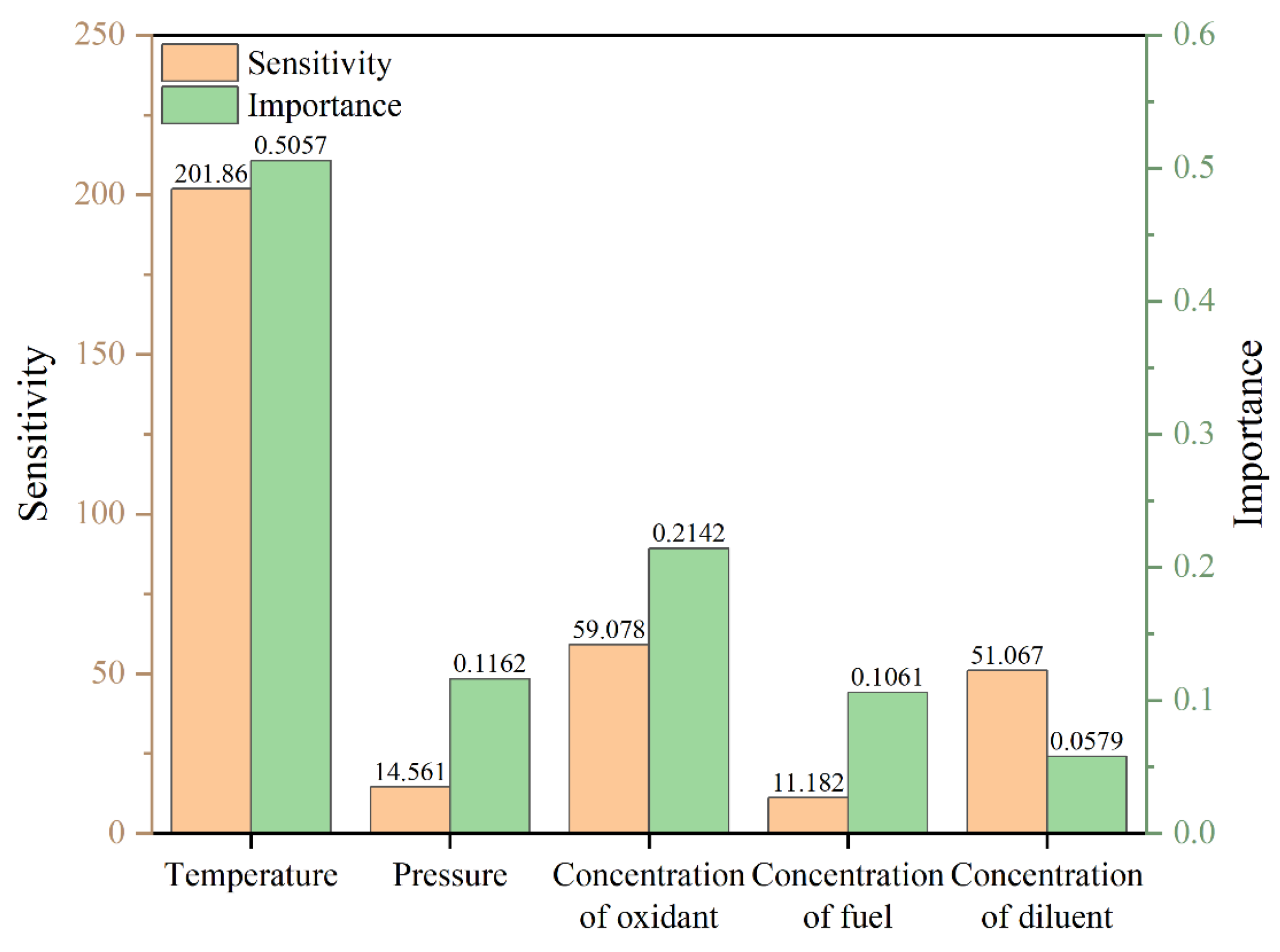
3.3.2. Importance and Sensitivity Analysis
To systematically investigate the effects of each input variable on the ignition delay time of RP-3 aviation fuel across different temperature ranges, this study conducted feature importance analysis and sensitivity analysis. For the importance analysis, the permutation importance method was employed. By performing multiple rounds of random shuffling of the input features and measuring the changes in model evaluation metrics, the quantitative "importance contribution" of each variable to the predicted output was assessed. For the sensitivity analysis, the benchmark point gradient analysis method was utilized. Using a typical representative point as the baseline, changes within ±50% were introduced, and the resulting output change rates were recorded. The first-order linear regression slope was then used as the sensitivity index. All results were statistically analyzed separately for the three temperature regions: low temperature (600–900 K), NTC (900–1100 K), and high temperature (1100–1500 K).
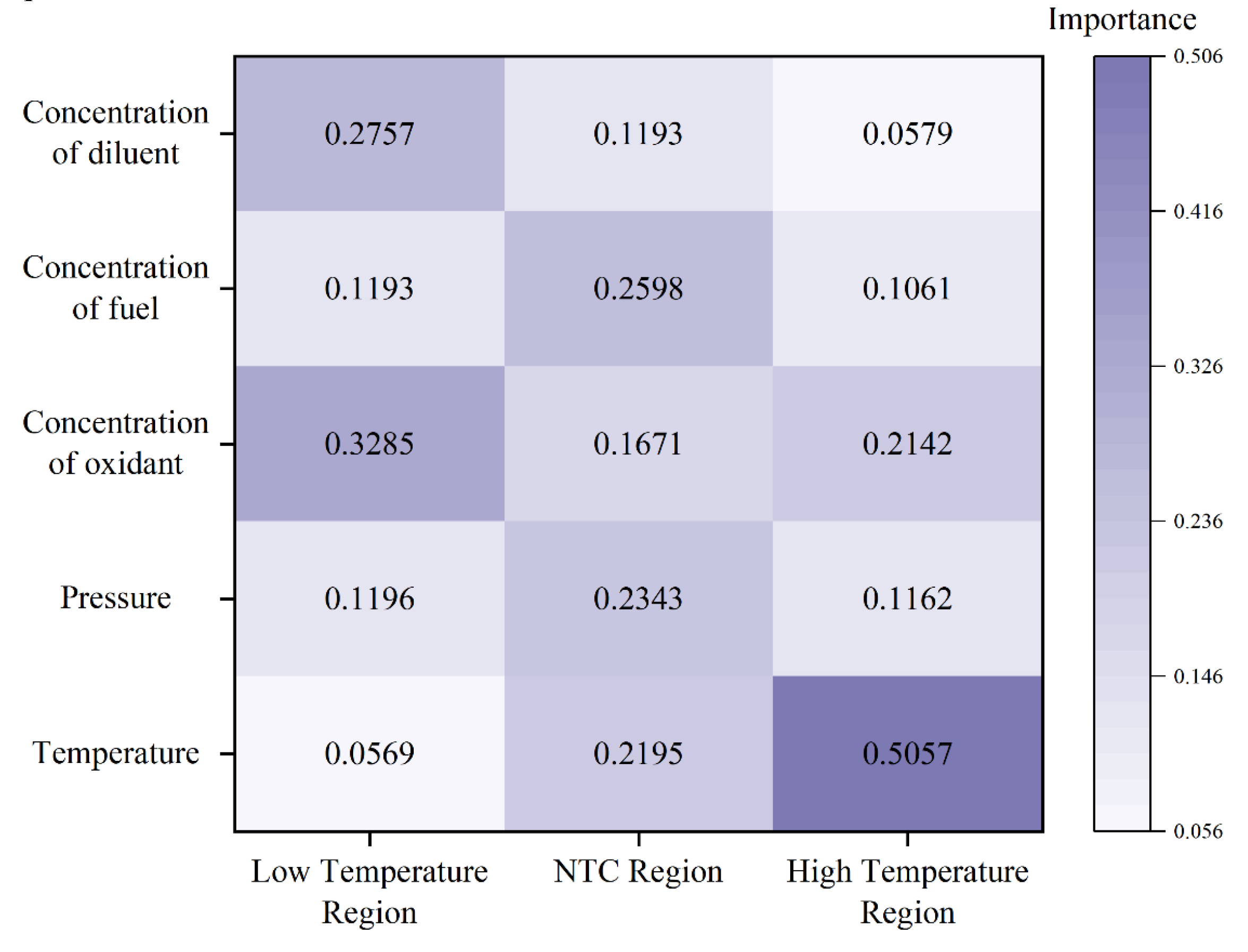
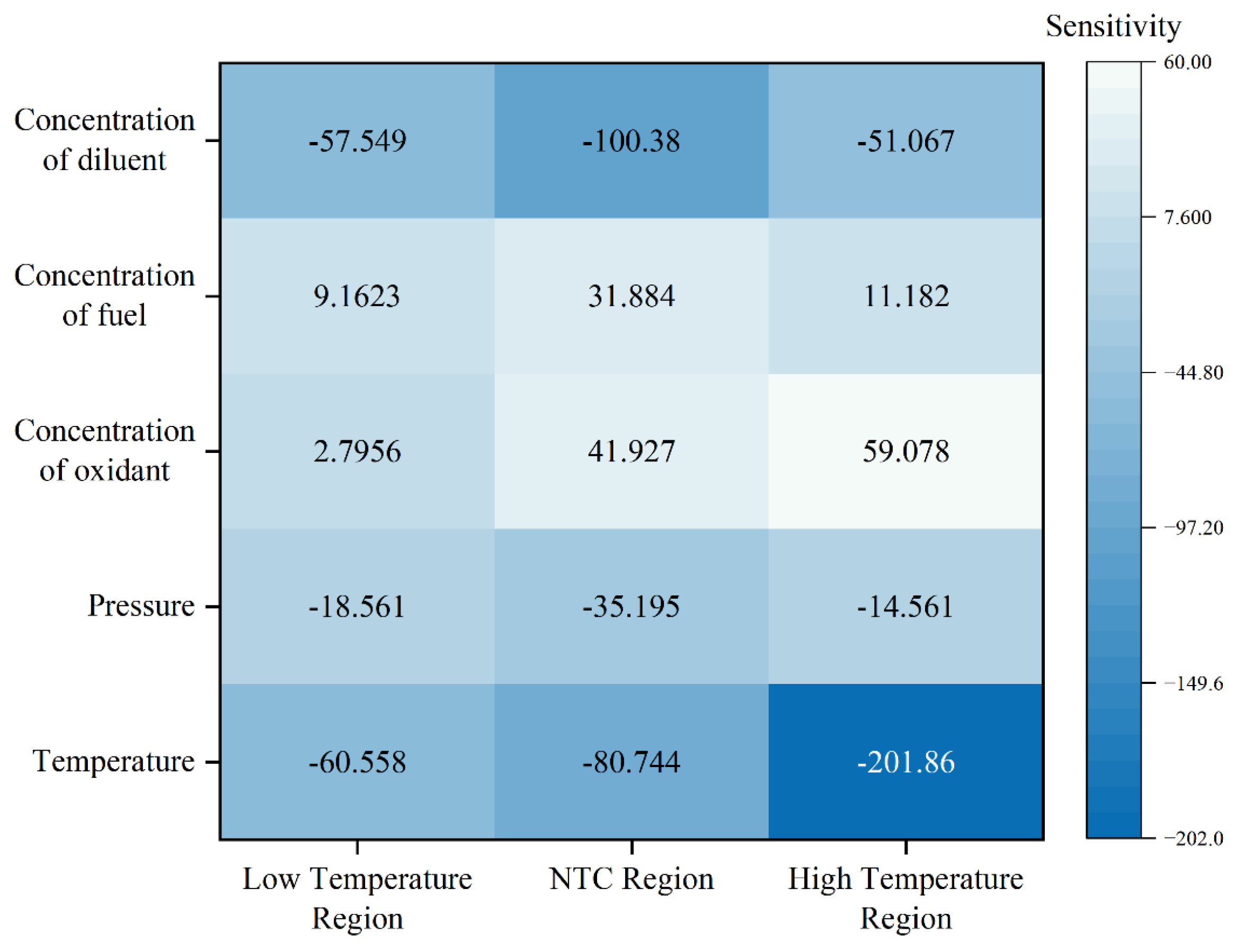
Figure 11.
Analysis of the Importance of Data.
Figure 12.
Analysis of the Sensitivity of Data.
From the importance analysis results presented in Figure 11, it is evident that in the low-temperature region, the molar fractions of the oxidant (0.3285) and the diluent (0.2757) exhibit the highest significance, surpassing other factors. This indicates that the molar fractions of the oxidant and diluent have a more pronounced effect on ignition delay time in the low-temperature region. Following these are the molar fraction of the fuel (0.1193) and the pressure of the mixture gas (0.1196), whereas the temperature (0.0569) has a relatively minor influence. In the medium-temperature region, the importance of the molar fractions of the oxidant and diluent decreases slightly to 0.1671 and 0.1193, respectively. Conversely, the importance of the molar fraction of the fuel and the pressure of the mixture gas increases, and the importance of the ignition temperature rises significantly to 0.2195. In the high-temperature region, the importance of the ignition temperature further increases to 0.5057, while the significance of other factors diminishes, suggesting that at high temperatures, the ignition temperature plays a decisive role in determining the combustion reaction rate.
From the results of the sensitivity analysis presented in Figure 12, the ignition temperature exhibits pronounced negative sensitivity across all temperature regions (low-temperature region: -60.558, NTC region: -80.744, high-temperature region: -201.86). This indicates that an increase in temperature significantly reduces the ignition delay time, aligning with the principles of combustion kinetics. The diluent fraction also demonstrates negative sensitivity, with higher sensitivity observed in the NTC region (-100.38) and even greater sensitivity in the low-temperature region, suggesting that an increase in diluent concentration accelerates the reaction process. The sensitivity values of the mixture gas pressure are generally small but exhibit a negative trend, implying that increased pressure facilitates a reduction in ignition delay time, consistent with the model's predictive capability discussed in Section 3.3.1. Both the fuel mole fraction and oxidant mole fraction display positive sensitivity, indicating that increases in these fractions tend to extend the ignition delay time, particularly in the high-temperature region, where the fuel mole fraction reaches its maximum sensitivity value (59.078).
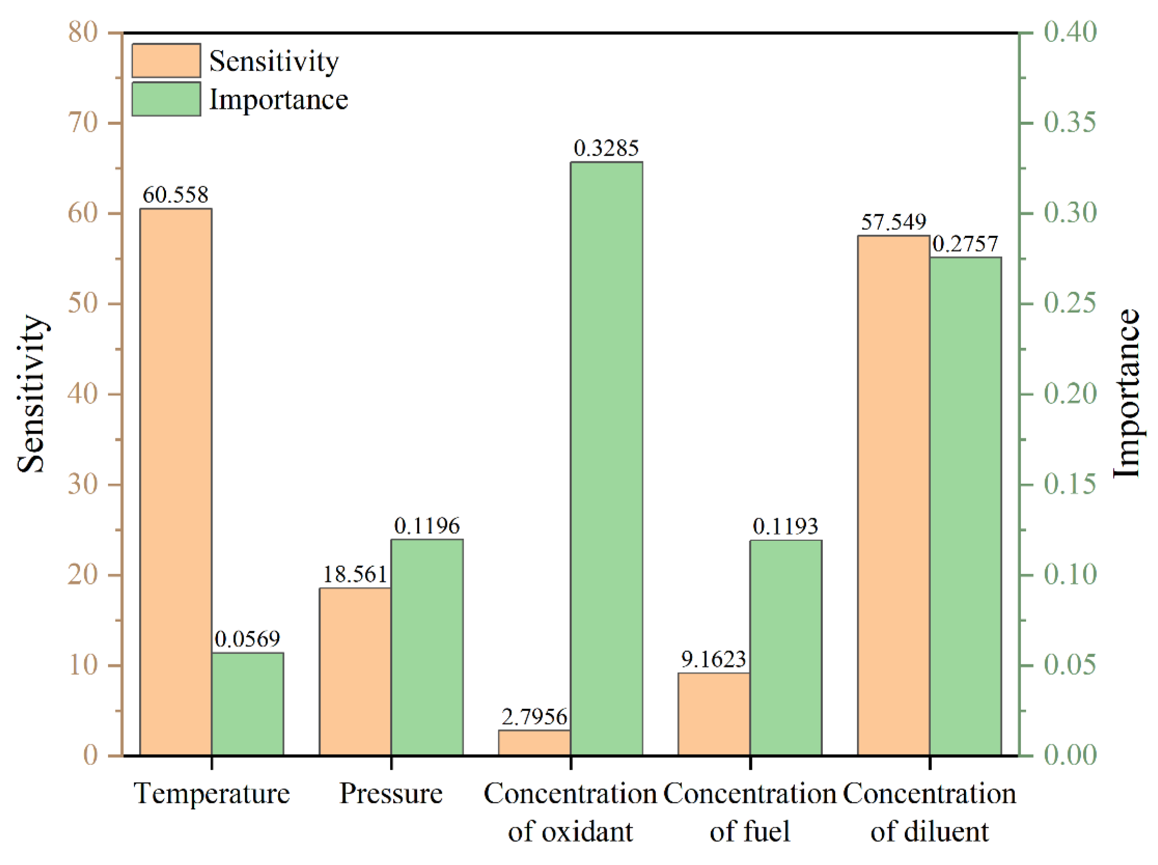
Figure 13.
The distribution of sensitivity and importance in the low-temperature region.
To visually display the data sensitivity and importance in the low-temperature region, the NTC region, and the high-temperature region, we plotted the histogram as shown in Figure 13,Figure 14 and Figure 15 after taking the absolute value of the sensitivity coefficient and the importance coefficient.
In the low-temperature region, the ignition temperature exhibits relatively high sensitivity but limited importance, meaning that while local variations can substantially impact ignition delay time, its overall contribution remains restricted. Both the importance and sensitivity of mixture gas pressure are low, whereas the oxidant mole fraction demonstrates high importance but low sensitivity, reflecting its role in governing global reaction dynamics. The diluent mole fraction is characterized by both high importance and sensitivity, making it the primary control factor for low-temperature ignition characteristics. In contrast, the influence of the fuel mole fraction in this region is minimal, likely due to its restricted variation range and weak effect on initial free radical generation.
In the NTC region, the importance and sensitivity of ignition temperature increase markedly, becoming the most critical control variable, consistent with the highly temperature-sensitive reaction mechanisms observed in this region. Mixture gas pressure shows high importance but low sensitivity, indicating that while its overall influence is significant, local changes have limited effects. The oxidant mole fraction in the NTC region exhibits moderate levels of both importance and sensitivity. Although the diluent mole fraction has low importance, it displays the highest sensitivity, underscoring its crucial regulatory role in free radical concentration and heat release rate. Finally, the fuel mole fraction exerts a substantial macroscopic influence but exhibits low sensitivity to local changes.
In the high-temperature regime, the ignition temperature retains its critical importance and sensitivity, governing the variation in ignition delay. During this interval, the mole fraction of the oxidant remains at a moderate level. In contrast, the mixture gas pressure, the mole fraction of the diluent, and the mole fraction of the fuel exhibit low levels of importance and sensitivity, suggesting that in the rapid oxidation process dominated by high temperatures, the impact of these variables on ignition delay time is further diminished. Overall, the variations across different temperature intervals indicate that fuel ignition delay characteristics are regulated by the interplay of multiple factors, and this regulatory mechanism exhibits pronounced stage-dependent behavior with changing temperature. These findings not only elucidate the temperature-dependent influence of each input parameter on ignition delay time but also furnish a theoretical foundation for subsequent combustion optimization and ignition control strategy development.
4. Discussion
This paper focuses on the prediction of the Ignition Delay Time (IDT) of RP-3 aviation kerosene and systematically evaluates the impact of different gradient descent algorithms, hidden layer structures, and activation function combinations on the model's predictive performance. The following principal conclusions are drawn:
Through comparative analysis of double-hidden-layer and triple-hidden-layer neural network structures across various neuron intervals, it is found that the triple-hidden-layer structure outperforms the double-hidden-layer one in terms of overall fitting performance, error control, and stability. Within the [15-35] neuron interval, R² can reach above 0.958, with the minimum values of MAPE and MAE being 2.77% and 0.0679, respectively, demonstrating excellent fitting and generalization capabilities. Experimental results indicate that the conjugate gradient descent method achieves optimal fitting performance (R²= 0.99705) in the triple-hidden-layer structure with a neuron distribution of [21 17 19], where MAPE is as low as 1.2%. This confirms the superiority of this gradient descent algorithm in nonlinear fitting tasks involving multiple input variables.
Under various equivalence ratios (φ= 1.0, 1.5, 2.0) and pressure conditions (10–20 bar), the prediction outcomes exhibit high consistency with the experimental results. Specifically, under medium equivalence ratios and medium-to-low pressure conditions, the predicted data points nearly perfectly align with the actual measurements, indicating excellent generalization and robustness of the model.
In the low-temperature region, the diluent mole fraction exhibits an importance value of 0.2757 and a sensitivity of -57.549, whereas the temperature sensitivity is -60.558 with relatively lower importance (0.0569). In the NTC region, temperature demonstrates an importance of 0.2195 and a sensitivity of -145.6, while the diluent shows the highest sensitivity (-140.5). The ambient pressure has an importance of 0.2237 but relatively low sensitivity (-80.744). In the high-temperature region, temperature dominates with an importance of 0.5057 and a sensitivity of -201.86, while the oxidant mole fraction exhibits medium-level importance and sensitivity. Significant differences exist in the distribution of importance and sensitivity of input variables regarding ignition delay time across different temperature regions. Temperature consistently acts as the dominant factor, while the effects of the mole fractions of diluent, oxidant, and fuel vary across regions. These findings reveal the temperature dependence and multi-factor coupling mechanism underlying RP-3 ignition delay characteristics, providing a theoretical foundation for modeling aviation fuel combustion and optimizing ignition control strategies.
Author Contributions
Wenbo Liu: Visualization, Writing–original draft, Investigation, Methodology, Writing–review and editing, Conceptualization, Supervision.;Zhirui Liu: Supervision, Writing–review and editing, Data curation, Formal Analysis, Writing–review and editing. Hongan Ma: Data curation, Validation, Writing–review and editing.
Funding
This research received no external funding
Data Availability Statement
The raw data supporting the conclusion of this article will be made available by the authors, without undue reservation.
Conflicts of Interest
The authors declare that they have no known competing financial interests or personal relationships that could have influenced the research presented in this manuscript.
Abbreviations
The following abbreviations are used in this manuscript:
| IDT | Ignition Delay Time |
| BP | Back Propagation |
| R² | Coefficient of Determination |
| MAPE | Mean Absolute Percentage Error |
| MAE | Mean Absolute Error |
| RMSE | Root Mean Squared Error |
| φ | Equivalence Ratios |
| P | Pressure |
| NTC | Negative Temperature Coefficient |
| CVCB | Constant Volume Combustion Bomb |
| RCM | Rapid Compression Machine |
| LIF | Laser-Induced Fluorescence |
| DNN | Deep feedforward Neural Network |
| RF | Random Forest |
| SVM | Support Vector Machine |
| CNNs | Convolutional Neural Networks |
| LSTMs | Long Short-Term Memory Networks |
| SHAP | SHapley Additive exPlanations |
| SGD | Standard Gradient Descent |
| MGD | Momentum Gradient Descent |
| AGA | Adaptive Gradient Algorithm |
| RPROP | Resilient Backpropagation |
| CGD | Conjugate Gradient Descent |
References
- Zeng W, Zou C, Yan T, et al. High-temperature ignition of ammonia/methyl isopropyl ketone: A shock tube experiment and a kinetic model[J]. Combustion and Flame, 2025, 276: 114004.
- Dai L, Liu J, Zou C, et al. Shock tube experiments and numerical study on ignition delay times of ammonia/oxymethylene ether-2 (OME2) mixtures[J]. Combustion and Flame, 2024, 270: 113783.
- Lin Q, Zou C, Dai L. High temperature ignition of ammonia/di-isopropyl ketone: A detailed kinetic model and a shock tube experiment[J]. Combustion and Flame, 2023, 251: 112692.
- Qu Y, Zou C, Xia W, et al. Shock tube experiments and numerical study on ignition delay times of ethane in super lean and ultra-lean combustion[J]. Combustion and Flame, 2022, 246: 112462.
- Reyes M, Tinaut F V, Andrés C, et al. A method to determine ignition delay times for Diesel surrogate fuels from combustion in a constant volume bomb: Inverse Livengood–Wu method[J]. Fuel, 2012, 102: 289-298.
- Wu Y, Liu Y, Tang C, et al. Ignition delay times measurement and kinetic modeling studies of 1-heptene, 2-heptene and n-heptane at low to intermediate temperatures by using a rapid compression machine[J]. Combustion and Flame, 2018, 197: 30-40.
- De Toni A R, Werler M, Hartmann R M, et al. Ignition delay times of Jet A-1 fuel: Measurements in a high-pressure shock tube and a rapid compression machine[J]. Proceedings of the Combustion Institute, 2017, 36(3): 3695-3703.
- Ramalingam A, Fenard Y, Heufer A. Ignition delay time and species measurement in a rapid compression machine: A case study on high-pressure oxidation of propane[J]. Combustion and Flame, 2020, 211: 392-405.
- Mao Y, Yu L, Wu Z, et al. Experimental and kinetic modeling study of ignition characteristics of RP-3 kerosene over low-to-high temperature ranges in a heated rapid compression machine and a heated shock tube[J]. Combustion and Flame, 2019, 203: 157-169.
- Schulz C, Sick V. Tracer-LIF diagnostics: Quantitative measurement of fuel concentration, temperature and fuel/air ratio in practical combustion systems[J]. Progress in Energy and Combustion Science, 2005, 31(1): 75–121.
- Shah Z A, Marseglia G, De Giorgi M G. Predictive models of laminar flame speed in NH3/H2/O3/air mixtures using multi-gene genetic programming under varied fuelling conditions[J]. Fuel, 2024, 368: 131652.
- Wang Y, Zhou X, Liu L. Study on the mechanism of the ignition process of ammonia/hydrogen mixture under high-pressure direct-injection engine conditions[J]. International Journal of Hydrogen Energy, 2021, 46(78): 38871-38886.
- Yamada S, Shimokuri D, Shy S, et al. Measurements and simulations of ignition delay times and laminar flame speeds of nonane isomers[J]. Combustion and Flame, 2021, 227: 283-295.
- Mao G, Zhao C, Yu H. Optimization of ammonia-dimethyl ether mechanisms for HCCI engines using reduced mechanisms and response surface methodology[J]. International Journal of Hydrogen Energy, 2025, 100: 267-283.
- Song T, Wang C, Wen M, et al. Combustion mechanism study of ammonia/n-dodecane/n-heptane/EHN blended fuel[J]. Applications in Energy and Combustion Science, 2024, 17: 100241.
- Gong Z, Feng L, Wei L, et al. Shock tube and kinetic study on ignition characteristics of lean methane/n-heptane mixtures at low and elevated pressures[J]. Energy, 2020, 197: 117242.
- Kelly M, Bourque G, Hase M, et al. Machine learned compact kinetic model for liquid fuel combustion[J]. Combustion and Flame, 2025, 272: 113876.
- Zhang H, Hu Y, Liu W, et al. Update of the present decomposition mechanisms of ammonia: A combined ReaxFF, DFT and chemkin study[J]. International Journal of Hydrogen Energy, 2024, 90: 557-567.
- Gong Z, Feng L, Li L, et al. Shock tube and kinetic study on ignition characteristics of methane/n-hexadecane mixtures[J]. Energy, 2020, 201: 117609.
- Wu Y, Li Y, Zhang L. Data-driven modeling of ignition delay time using artificial neural networks[J]. Energy, 2020, 193: 116726.
- Liu Y, Chen Y. Application of neural network in combustion characteristics prediction of alternative aviation fuels[J]. Fuel, 2021, 294: 120576.
- Wang H, Wang Z, Zhang Y. Prediction of ignition delay times of surrogate jet fuels using machine learning methods[J]. Fuel, 2022, 308: 122048.
- Zhang C, Lin Y. Ignition delay prediction using deep learning with convolutional neural networks[J]. Combustion Theory and Modelling, 2022, 26(1): 135–150.
- Patel R, Saxena P. Sequence modeling of ignition delay using LSTM networks for real-time combustion diagnostics[J]. Applied Energy, 2023, 345: 121042.
- Wang J, Li M, Zhou L, et al. Ignition delay prediction of RP-3 aviation kerosene using neural networks trained on shock tube data[J]. Aerospace Science and Technology, 2021, 114: 106795.
- Ji W, Su X, Pang B, et al. SGD-based optimization in modeling combustion kinetics: Case studies in tuning mechanistic and hybrid kinetic models[J]. Fuel, 2022, 324: 124560.
- Zhang L, Ma Y, Li S. Improving generalization of neural network-based ignition delay prediction using transfer learning and data augmentation[J]. Combustion and Flame, 2020, 215: 392–401.
- Zhao Y, Xu M. Feature sensitivity and interpretability analysis of neural network predictions in combustion systems[J]. Fuel, 2022, 314: 123089.
- Chen B H, Liu J Z, Yao F, et al. Ignition delay characteristics of RP-3 under ultra-low pressure (0.01–0.1 MPa)[J]. Combustion and Flame, 2019, 210: 126-133.
- Liu J, Hu E, Yin G, et al. An experimental and kinetic modeling study on the low-temperature oxidation, ignition delay time, and laminar flame speed of a surrogate fuel for RP-3 kerosene[J]. Combustion and Flame, 2022, 237: 111821.
- Liu J, Hu E, Zeng W, et al. A new surrogate fuel for emulating the physical and chemical properties of RP-3 kerosene[J]. Fuel, 2020, 259: 116210.
- Mao Y, Yu L, Wu Z, et al. Experimental and kinetic modeling study of ignition characteristics of RP-3 kerosene over low-to-high temperature ranges in a heated rapid compression machine and a heated shock tube[J]. Combustion and Flame, 2019, 203: 157-169.
- Yang Z Y, Zeng P, Wang B Y, et al. Ignition characteristics of an alternative kerosene from direct coal liquefaction and its blends with conventional RP-3 jet fuel[J]. Fuel, 2021, 291: 120258.
- Zhang C, Li B, Rao F, et al. A shock tube study of the autoignition characteristics of RP-3 jet fuel[J]. Proceedings of the Combustion Institute, 2015, 35(3): 3151-3158.
Figure 1.
Schematic representation of the BP neural network architecture.
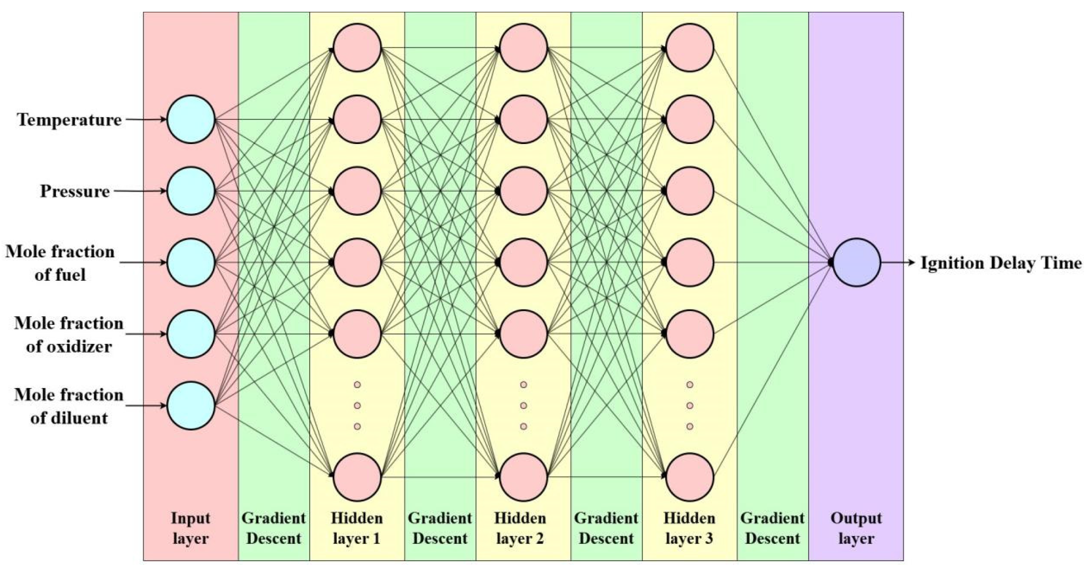
Figure 2.
Performance Comparison of Two-Hidden-Layer Structures Across Different Neuron Intervals.
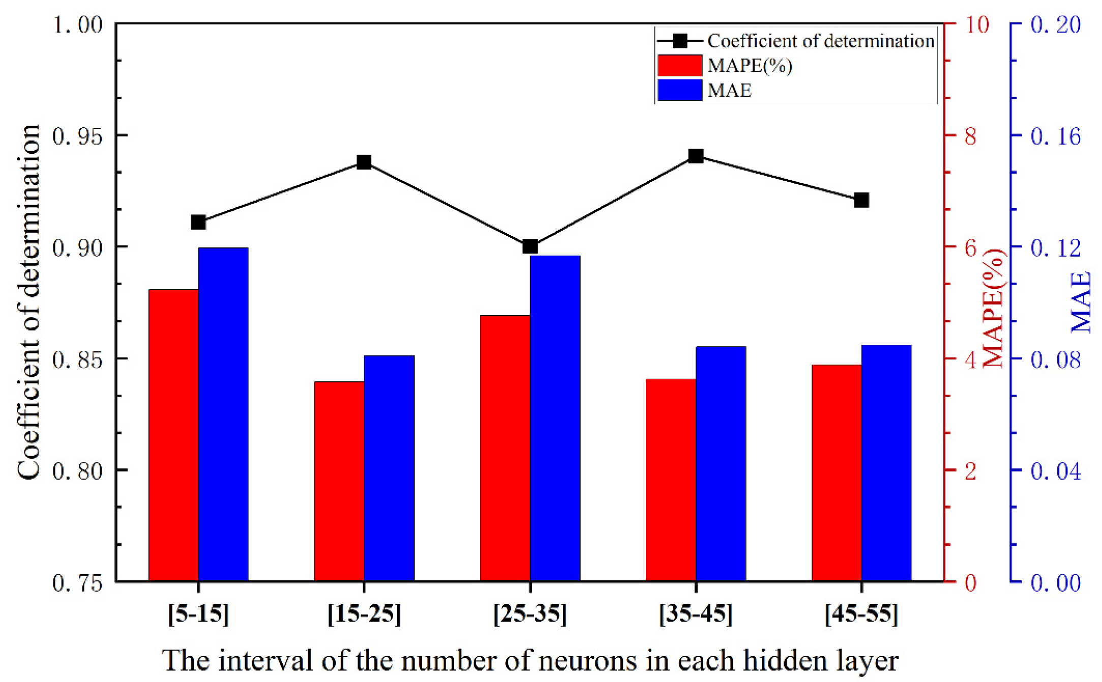
Figure 3.
Performance Comparison of the Three-Hidden-Layer Structure Across Different Neuron Intervals.
Figure 3.
Performance Comparison of the Three-Hidden-Layer Structure Across Different Neuron Intervals.
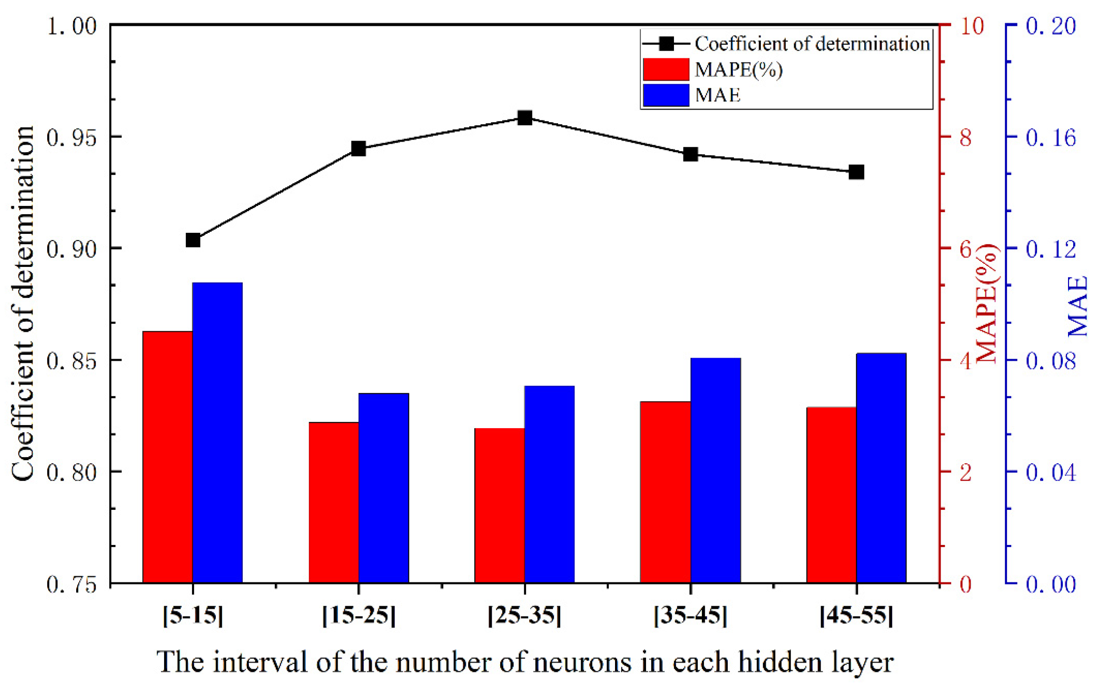
Figure 4.
MAE values obtained from various gradient descent algorithms.
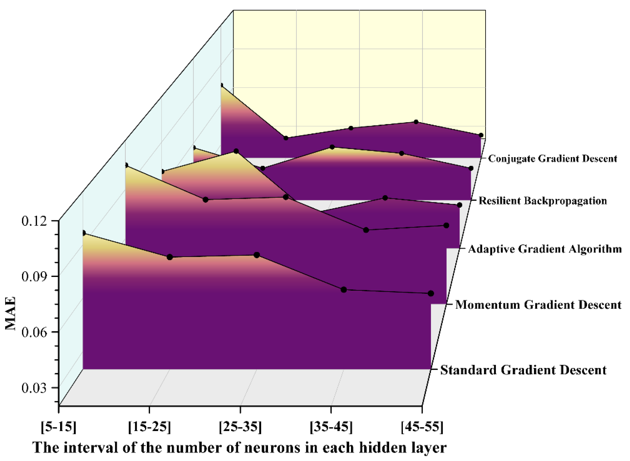
Figure 5.
R² values obtained from various gradient descent algorithms.
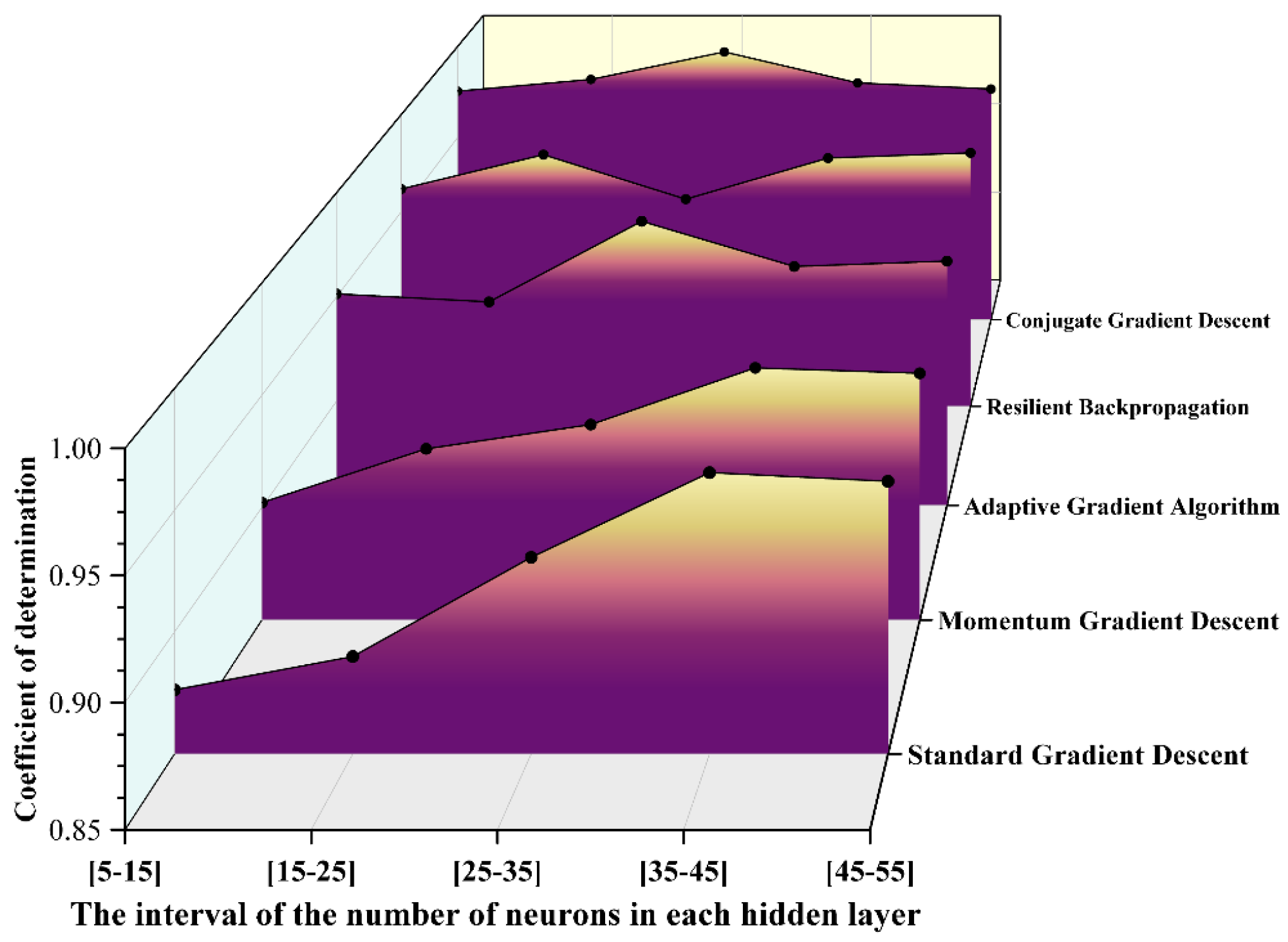
Figure 6.
MAPE values obtained from various gradient descent algorithms.
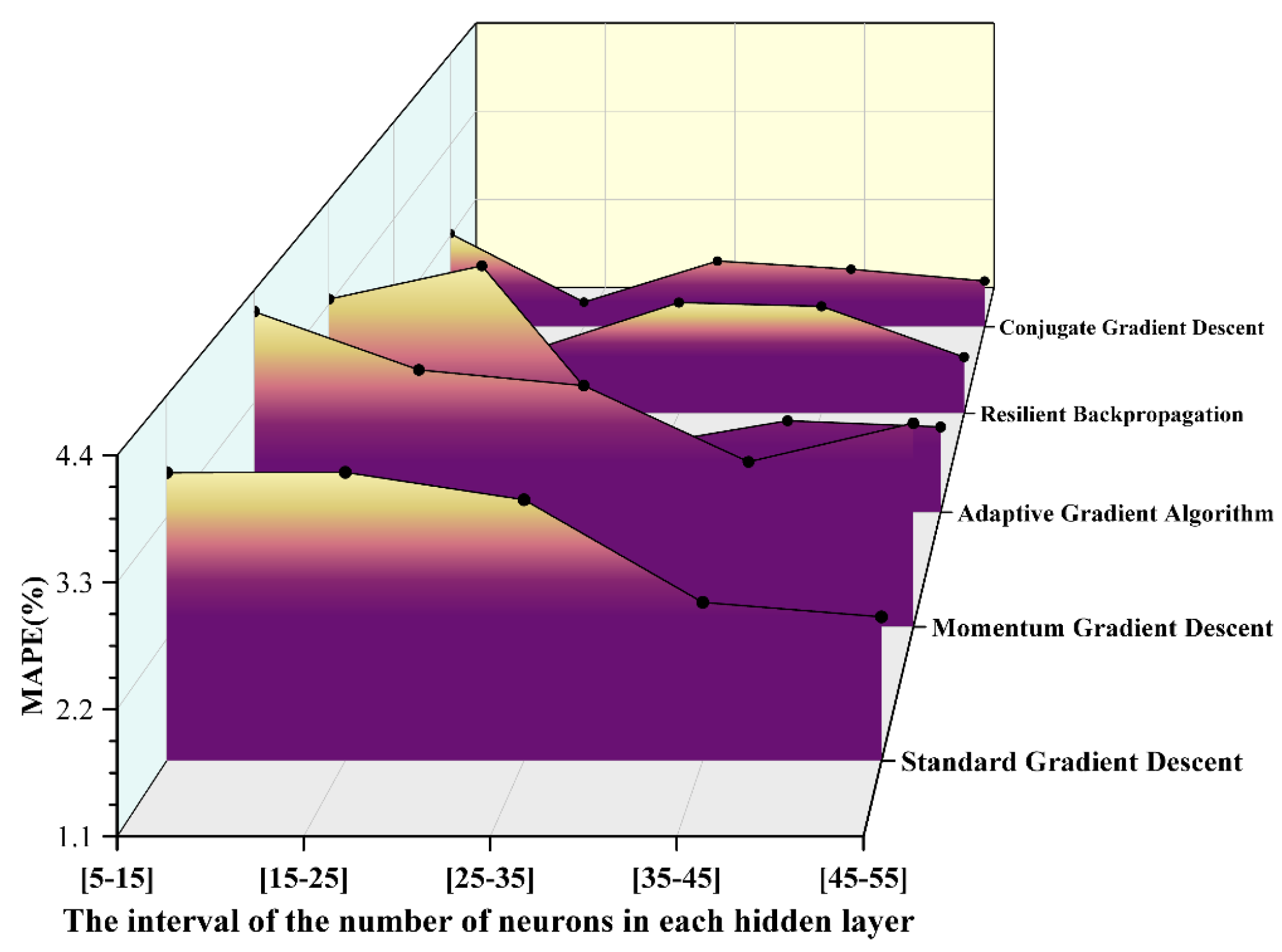
Figure 7.
Comparison of evaluation indicators of five different gradient descent algorithms.
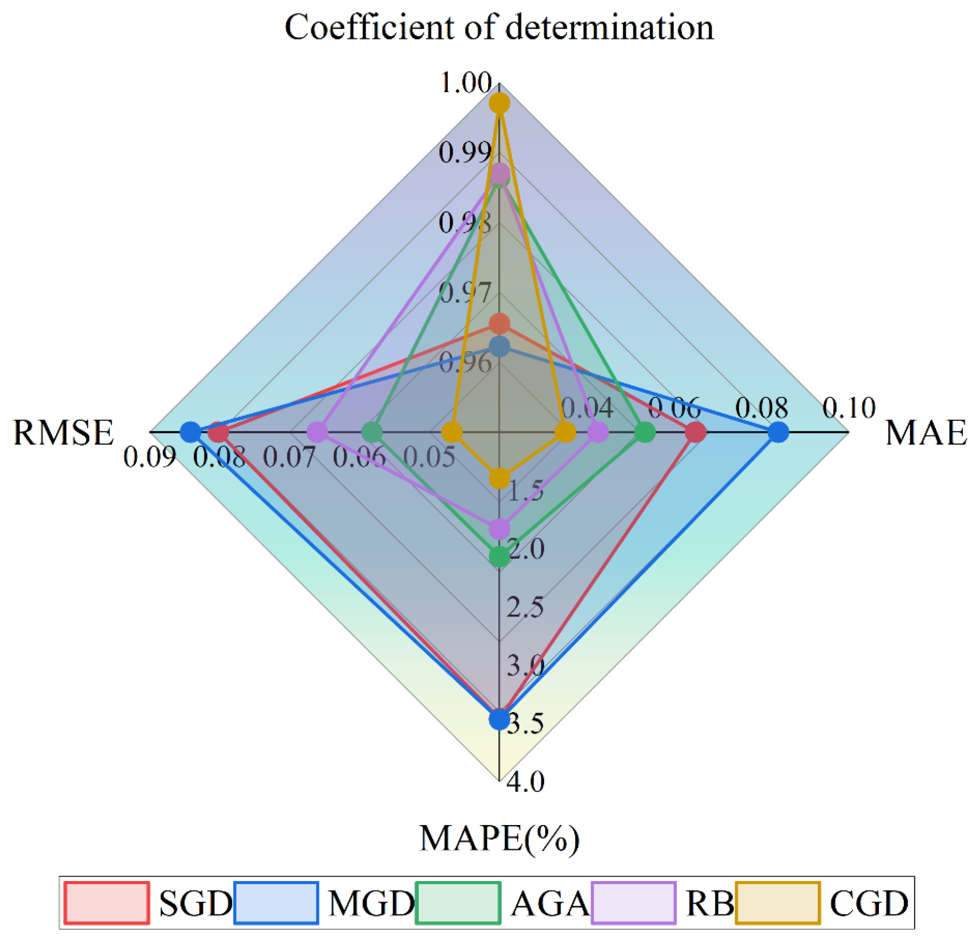
Figure 8.
Data prediction when the equivalence ratio is 1 and the pressures are 20 bar, 15 bar, and 10 bar respectively.
Figure 8.
Data prediction when the equivalence ratio is 1 and the pressures are 20 bar, 15 bar, and 10 bar respectively.
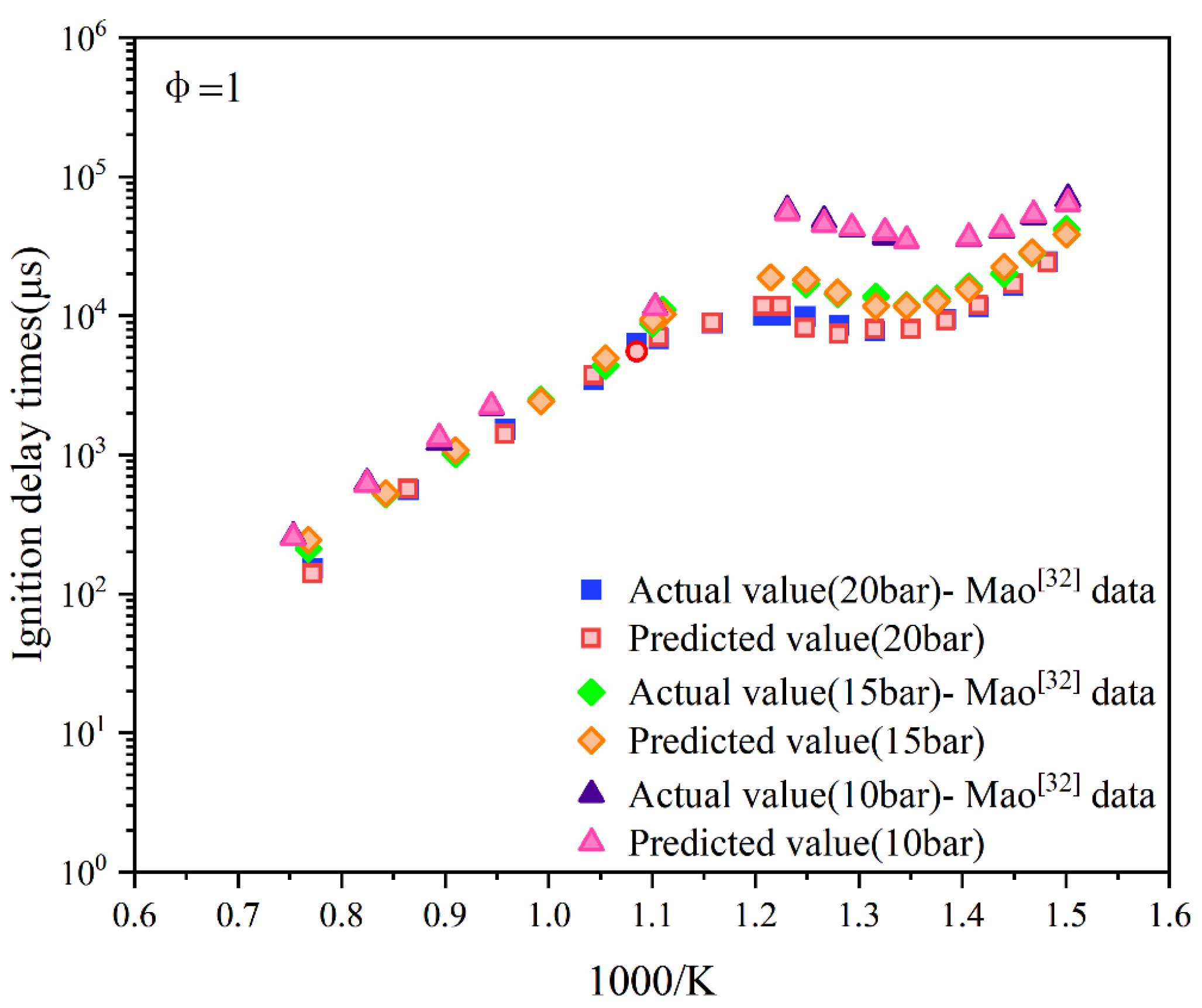
Figure 9.
Data prediction when the equivalence ratio is 1.5 and the pressures are 20 bar, 15 bar, and 10 bar respectively.
Figure 9.
Data prediction when the equivalence ratio is 1.5 and the pressures are 20 bar, 15 bar, and 10 bar respectively.
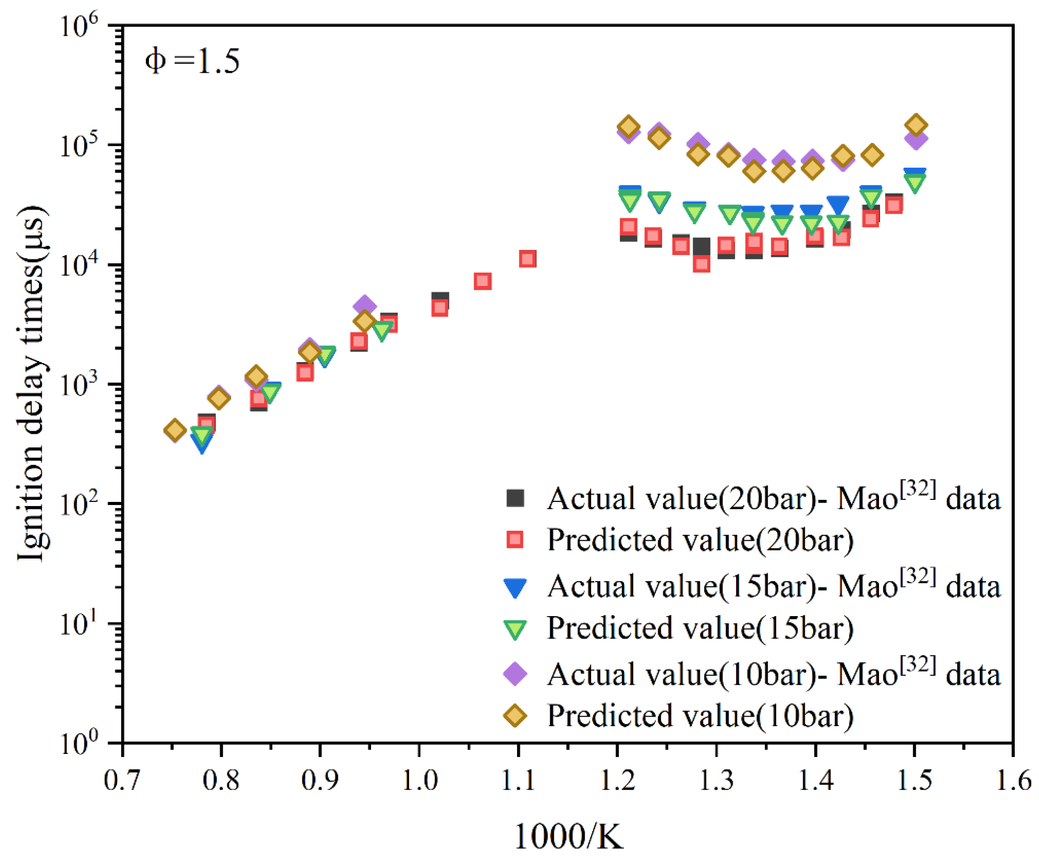
Figure 10.
Data prediction when the equivalence ratio is 2 and the pressures are 20 bar and 10 bar respectively.
Figure 10.
Data prediction when the equivalence ratio is 2 and the pressures are 20 bar and 10 bar respectively.
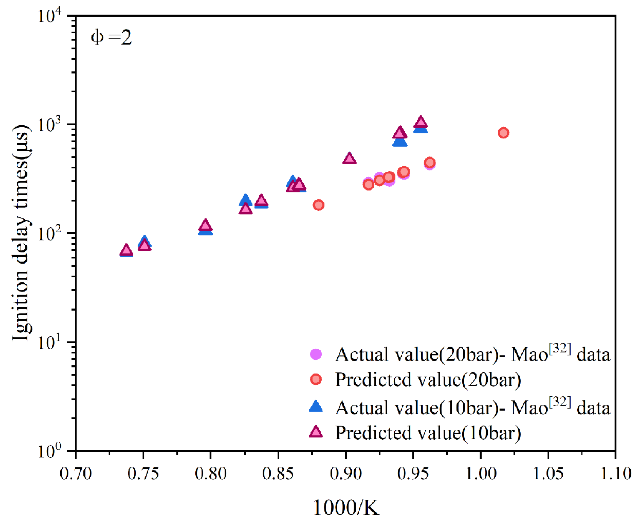
Figure 14.
The distribution of sensitivity and importance in the NTC region.
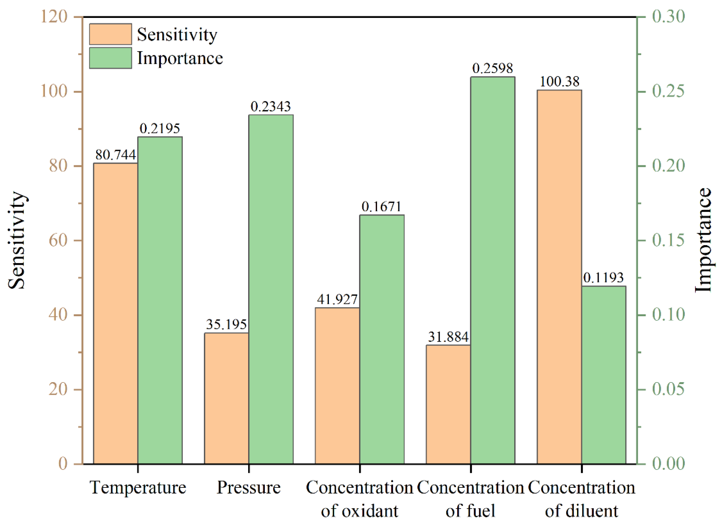
Figure 15.
The distribution of sensitivity and importance in the high-temperature region.
Disclaimer/Publisher’s Note: The statements, opinions and data contained in all publications are solely those of the individual author(s) and contributor(s) and not of MDPI and/or the editor(s). MDPI and/or the editor(s) disclaim responsibility for any injury to people or property resulting from any ideas, methods, instructions or products referred to in the content. |
© 2025 by the authors. Licensee MDPI, Basel, Switzerland. This article is an open access article distributed under the terms and conditions of the Creative Commons Attribution (CC BY) license (http://creativecommons.org/licenses/by/4.0/).
Copyright: This open access article is published under a Creative Commons CC BY 4.0 license, which permit the free download, distribution, and reuse, provided that the author and preprint are cited in any reuse.


