
Submitted:
06 May 2025
Posted:
07 May 2025
You are already at the latest version
Abstract
For applications in many fields, ordinal patterns are a successful tool. Here we address the need for theoretical models. A paradigmatic example shows that a model for frequencies of ordinal patterns can be determined without any numerical values. We specify the important concept of stationary order and the fundamental problems to be solved in order to establish a genuine statistical methodology for ordinal time series.
Keywords:
ordinal pattern
; stochastic process
; time series
; permutation entropy
MSC: 37A35; 62M10; 60G07
1. Introduction
1.1. Contents of the Paper
In this introductory section, we introduce the basic concepts in a brief manner. For more detail and background, we refer to ([1] Section II) and [2,3,4,5,6,7]. A new point is the visualization of the distribution of ordinal patterns as refining ordinal histogram in Section 1.4. The main topic of the paper is explained in Section 1.6. Order-related properties of processes, in particular order self-similarity, are introduced in Section 1.7.
Section 2 deals with a paradigmatic example of an ordinal process which has no numerical values. The construction is algorithmic and intuitive, and the probabilities for patterns of length 3 are the same as for Brownian motion. Unfortunately, the example is not self-similar and not relevant for applications. We conjecture that there is a self-similar modification.
The final Section 3 gives a more technical outline of a possible theory of ordinal processes. We construct stationary ordinal processes without using numerical values. Order self-similarity remains an open problem.
1.2. Permutations as Patterns in Time Series
A permutation of length m is a one-to-one mapping from the set onto itself. We write for and Thus means However, we do not need mapping properties of permutations like composition. We just consider the graph of as a geometric pattern - an ordinal pattern.
With we denote a time series of length It is also a mapping, assigning to the time points the values For m time points between 1 and T we consider the pattern of corresponding values. We define
In other words, the correspondence is strictly monotonous. This is very intuitive. The pattern can be determined from the time series by calculating ranks: is the number of time points for which
1.3. Pattern Frequencies in Time Series
Instead of arbitrary we study equally spaced time points We call m the length and d the delay or lag of the pattern. We always take and mainly consider and However, we vary d as much as possible.
Ordinal pattern analysis is a statistical method. We fix a length m and determine relative frequencies of all patterns of length for various delays We divide the number of occurences of by the number of time points where could occur.
These frequencies are the basic parameters of ordinal time series analysis. They can be combined to calculate permutation entropy, persistence, and other important parameters [1,2,3,4,5,6,7].
1.4. Visualization of Pattern Frequencies by an Ordinal Histogram
This paper is not about parameters like entropy. It studies models for all pattern frequencies together. For this reason, we here introduce a graphical method to subsume the pattern frequencies for fixed d in a kind of density function. The permutations are assigned subintervals of as follows: We draw bars over which have area For we note that (neglecting a possible tiny error due to the last value for in (2)). We choose so that their union is Then we again draw bars with area The same is done for In this way, the histogram for is a refinement of the histogram for Sukzessive refinements can be obtained for although the length of the time series will rarely allow reliable estimates for This arrangement of permutations is called hierarchical order. Details will be given in Section 3.4. As Figure 1 shows for a simulated time series, all pattern frequencies of a time series for a fixed d can be subsumed in this way by a sequence of refining histograms, or in the limit by a kind of density function.
The process chosen for Figure 1 is an AR(1) model with exponential noise: where the are independent uniformly distributed random numbers in Due to the asymmetry of the noise distribution, Sukzessive decreasing steps are frequent: and We cannot explain why 2143 is the permutation with the second largest frequency. However, an AR(1) model with coefficient has a short memory. For the patterns already have almost uniform frequencies. The models considered below are more uniform for and 3, but they provide interesting behavior also for large
The problem of this paper is to find typical ordinal histograms from a theoretical viewpoint. An important question is to find models where the histograms agree for all Two such models are known ([1] Section II.C): white noise, where the histogram is a constant function for all and Brownian motion, see Figure 3 below. We are looking for other models.
1.5. Stationary and Order Stationary Processes
In time series analysis, we do always assume that the given time series is an instance of a larger ensemble, called a stochastical process. The process represents the mechanism which generates the given time series and many other ones. We want to know the laws of this process. Formally, a stochastical process X is a sequence of real random variables on a probability space The time series x is a random choice from the ensemble
To find the laws of X from one single time series, we must assume that the distributions and dependencies of the do not change in time. Usually X is required to be stationary. That is, the m-dimensional distribution of does not depend on for all This assumption is very strong. When we study autocorrelation, we assume weak stationarity. That is, the mean and the covariance do not depend on t [8]. When we consider ordinal patterns, we assume a similar very weak stationarity assumption. It will be required throughout this paper.
Order stationarity. For a given pattern with length m and delay let
denote the probability that the process X shows pattern just after time We say that the process X is order stationary for patterns of length m if is the same value for all This should hold for all patterns of length m and all delays where is chosen much smaller than the length T of our time series.
Brownian motion (where and are independent increments with standard normal distribution for ) is an order stationary process which is not even weakly stationary. It is a basic model for financial time series. Note that the process X and the pattern probabilities are theoretical objects. The observed frequency is an estimate for and from the viewpoint of theory, the estimator formula (2) has nice properties [9,10,11,12,13]. The practical success of ordinal patterns indicates that the assumption of order-stationarity is at least approximately fulfilled in applications.
1.6. The topic of this paper.
There are plenty of well-studied stochastic processes: Gaussian processes, random walks, ARMA and GARCH processes, processes with long-range dependence [11,14] etc. Most of them are either stationary or have stationary (multidimensional) increments and so are order stationary. They are defined by arithmetical operations, however. This makes the rigorous study of ordinal pattern frequencies difficult although various interesting theorems could be derived [9,10,11,15,16]. Even for Brownian motion, exact frequencies of patterns can be determined only for [17]. Some of them are rational, some irrational. Frequencies for length 5 lead to integrals which can be only numerically calculated. On the whole, the impression is that ordinal patterns do not fit into the established theory of stochastic processes.
The only proper theoretical model for pattern frequencies is white noise, a process of independent and identically distributed random variables For each all permutations have the same probability for any delay This model was repeatedly used as null hypothesis for testing serial dependence of time series [1,12,13,18,19,20,21]. A greater variety of models is needed.
In this paper, we try to define ordinal random processes in a combinatorial way, directly by their ordinal pattern frequencies. We do not require normal distribution, we require no arithmetics, and we even do not need numerical values to compare objects and An algorithmic example in the next chapter will show that this is possible. In Section 3, we outline some technical concepts and basic statements for a theory of ordinal processes. This could be a first step towards finding more applicable ordinal models. Note that possible equality of values, an important problem in practice [21], plays no role in this paper: our models will only allow or but not
1.7. Symmetry and Independence Properties of Ordinal Processes
Of course it is not enough to just postulate pattern frequencies. Our models should also have nice properties. Here we list the ordinal version of some of the most common process properties. We start with symmetry in time and space [9].
A process X is reversible if the distributions of and agree for every In the ordinal version, it is reversible if the permutations and have the same pattern probability for every The process X is invariant under reversal of values if the distributions of and agree for every The ordinal version states that the permutations and have the same pattern probability for every
In both cases, the ordinal versions of symmetry are much weaker and much easier to check. These symmetry properties are often met in applications. As a consequence, the distribution of ordinal patterns of length 3 often has only one degree of freedom, since and the probabilities of the other four permutations agree. All Gaussian processes are symmetric in space and time [9,11,17].
A process X is said to be Markov if for any t and fixed the distributions of and are independent. In the ordinal version, this means that the appearance of patterns at times and respectively, are independent. Again, the ordinal property is weaker and easier to check. The Markov property appears in theory rather than in applications. It implies that which is too large to occur in practice, even in financial data.
Order self-similarity. The most important symmetry property in this paper is order self-similarity ([22] Section 6). A random process in continuous time, is said to be self-similar if there is an exponent such that in distribution, for each positive number r [23]. Such a process cannot be stationary, it must look similar to Brownian motion. The ordinal concept is weaker and much simpler.
A process X is said to be order self-similar for patterns π of length m if
This should hold for all patterns of length m and all delays where is chosen much smaller than the length T of our time series.
2. The Coin-Tossing Order—An Ordinal Process Without Values
2.1. Ranking Fighters by Their Strength
Ordinal patterns were derived from numerical values of a time series. Now we go the opposite way, as in the world of tennis or chess where players first pairwise compare each other and afterwards are assigned a rank or ELO score. Suppose there are four players in a tennis club. We design an algorithm to order them by strength. First B plays against Let us assume B wins. Then we write Now the next player C plays against the previous player If C wins, then by transitivity of order. If C loses, however, C must still play against Depending on the result, either or Now the last player D comes and plays first against the previous player and then against B and/or if the comparison is not yet determined by previous games and transitivity.
This procedure will be turned into a mathematical model. We want to construct a random order between objects which are not numbers. We follow the algorithm for tennis players, and replace each match by the toss of a fair coin. As a result we obtain a stochastic process like white noise or Brownian motion, on ordinal level only. It will be possible to determine pattern probabilities much better than for Brownian motion.
2.2. Definition of the Coin Tossing Order
Repeated toin cossing is a standard way to represent randomness. Take a simple random walk, for example, and write for our position at time Then and either or depending on the result of a coin throw at time In the present case, will denote objects, not necessarily numbers. We define a random order between the We throw a fair coin to decide whether or for any pair of integers Let us write 1 for `head’ and 0 for `tail’. Then our basic probability space is the space of all 0-1-sequences, where each coordinate is 0 or 1 with probability independently of all other coordinates. Formally,
where means and means for The important point is that will be disregarded when the order of and is already fixed by previous comparisons and transitivity.
The first coin decides the ordering of and Now suppose are already ordered. Then is compared to by considering the random numbers However, when the comparison is fixed by transitivity from the already defined ordering, then is disregarded - that coin need not be thrown.
The resulting random order will be called coin tossing order. It can be easily simulated. Figure 2 shows rank numbers of 500 consecutive objects in the middle of a simulated series of length The global rank numbers have strange discontinuities. Local rank numbers, obtained by comparing with the next 20 objects on the left and right, show a more familiar picture.
Problem. Is there a stochastic process with stationary increments which generates the coin tossing order?
2.3. Basic Properties of the Coin Tossing Order
Despite the erratic view of trajectories in Figure 2, it turns out that the coin-tossing order has the same ordinal pattern frequencies for length 3 as Brownian motion, for arbitrary In particular, it is order self-similar for patterns of length 3.
Theorem 1
(Basic properties of the coin tossing order).
- (i)
- The coin tossing order is stationary and has the ordinal Markov property.
- (ii)
- For any permutation π of length the pattern probability is with
- (iii)
- The pattern probabilities are invariant under time reversal and reversal of the values.
- (iv)
- For we have and for the other permutations of length 3.
Proof. (i): The order of depends on the random numbers in the same way as the order of depends on the Since both collections of random numbers have the same distribution, the pattern probabilities do not depend on and the defined random order is stationary. Moreover, the comparisons of with depend on random numbers with while the comparisons of with depend on with Since different are independent, this implies the ordinal Markov property.
(ii): is the number of coin flips needed to determine Given a permutation we determine the which are needed to define the occurence of in Of course and j runs in increasing order. For fixed the number is always used, and the other i are considered in decreasing order. Now consider some k with If this was determined by the random numbers and which were drawn before In that case is disregarded since follows from the transitivity of the order. Similar for However, if there is no between and then is needed to determine We shall call the energy of
(iii): First we consider Given we have to show that the time-reversed and spatially reversed permutations have the same energy For spatial reversal this directly follows from the definition (5) with `between’. For time reversal, we show that can also be determined backwards by considering the with decreasing and for fixed with increasing The point is that when we compare places we have already compared both j and i with all k between. So is needed only if no is between and Otherwise the order between and is already fixed, and is disregarded. This proves reversibility for
Now consider and some of length m which appears as pattern of The probability of this event is which may be different from We have to calculate from all `atom permutations’ of length for for which the order among the special m places agrees with the order of This would be a lot of work. However, since the reversed permutation of is composed of the reversed `atom permutations’, both in space and in time, we shall get the same pattern probability.
(iv): The spatial reversal invariance implies Then follows from the Markov property. The equality of the four other pattern frequencies is a consequence of the invariance under time and space reversal. □
2.4. Computer Work and Breakdown of Self-Similarity
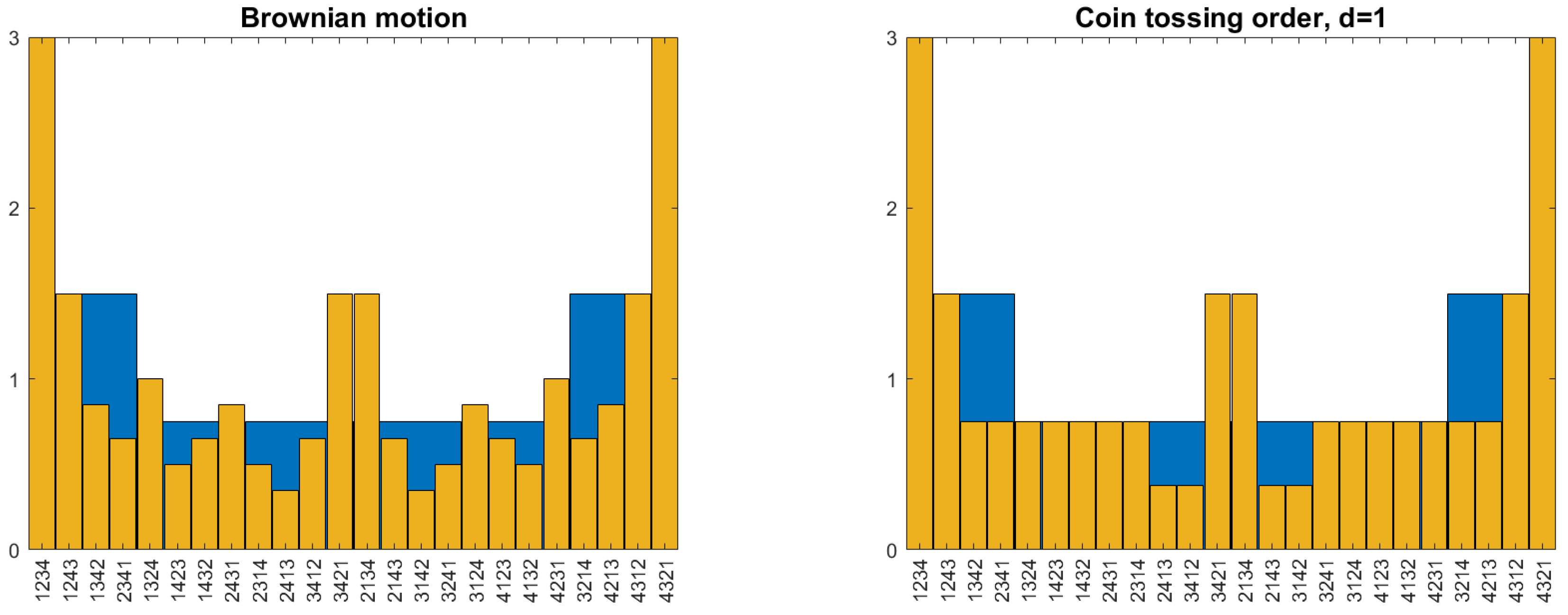
In Figure 3 we compare pattern probabilities of length 4 for Brownian motion and coin tossing order. Brownian motion looks more interesting since coin-tossing allows only the probabilities Our model is a first attempt, not recommended for applications. For length 3, the of the two processes agree and do not depend on according to Theorem 1. The figure shows that we must investigate patterns of length if we want to distinguish processes like these two. Moreover, Brownian motion is perfectly self-similar so that the probabilities of any length do not depend on d [23]. Is that also true for the coin tossing order?
Figure 3.
Probabilities of patterns of length 4 (brown) on top of those of length 3 (blue) for Brownian motion (left) and coin tossing order with (right). For length 3, the probabilities coincide.
Figure 3.
Probabilities of patterns of length 4 (brown) on top of those of length 3 (blue) for Brownian motion (left) and coin tossing order with (right). For length 3, the probabilities coincide.
The Equation (5) allows fast calculation of all pattern probabilities for and So we can determine for all permutations of length 4 and and 3 by adding the probabilities of `atom permutations’ of length 7 and 10, respectively, as sketched in the proof of Theorem 1, (iii). For we have to add cases for each permutation.
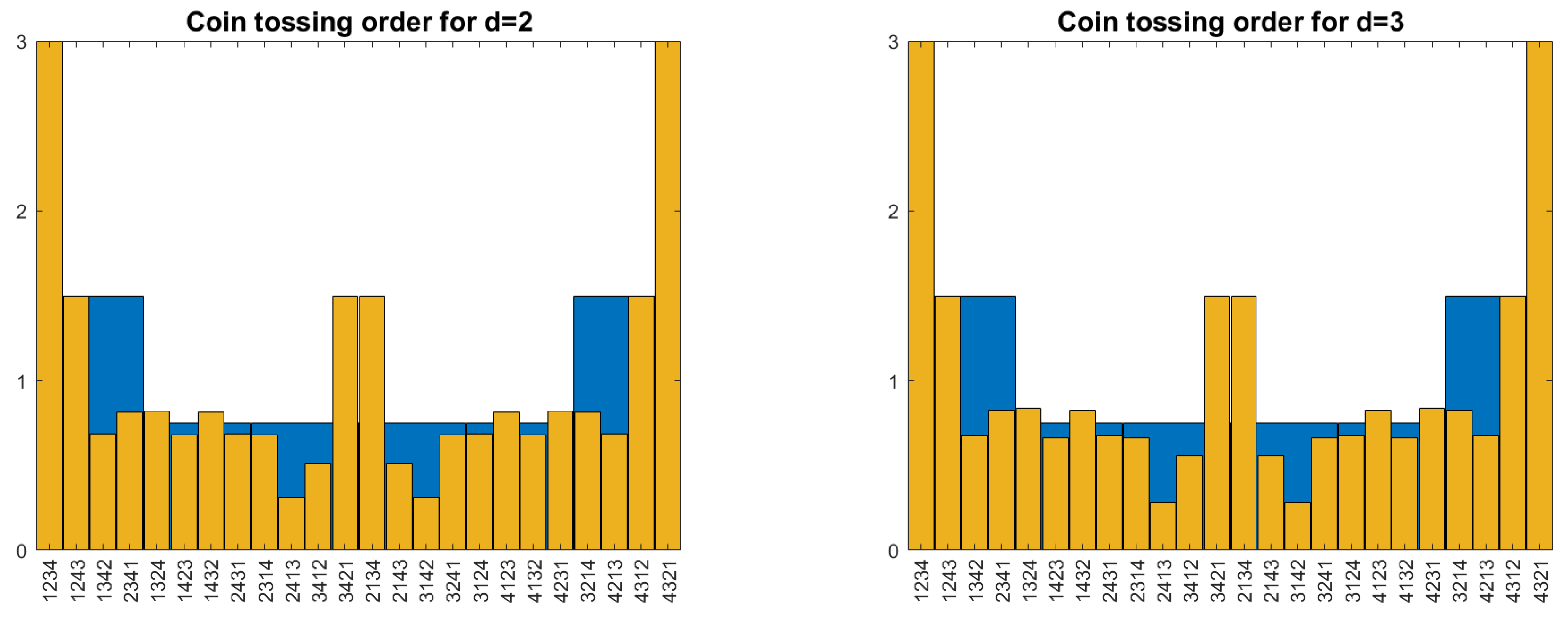
The result is shown in Figure 4. Unfortunately, order self-similarity breaks down for patterns of length 4. For we have while and However, the probabilities for or 3 can be taken as a new model which is nearer to self-similarity and looks not as artificial as coin tossing in Figure 3.
Problem. Let us define new pattern probabilities for What are the properties of Q ? Is there a limit for ?
The small difference between and in Figure 4 indicates fast convergence. The mere existence of an order self-similar limit would be interesting but not yet helpful. Brownian motion is already available as an order self-similar process. The merit of the coin tossing order is its algorithmic flavour, its connection with ranking. We look for an order self-similar model with an intuitive explanation.
Finally, let us consider the interpretation of as an energy function. Let and let denote the set of all permutations of length Let P denote the probability measure on given by the probabilities of coin tossing order. The permutation entropy [24] of using logarithms with base 2, is just the mean energy with respect to
For all other probability measures Q on the permutation entropy is smaller than the mean energy, see ([25] Chapter 1). Thus P is a so-called Gibbs measure on
Problem. Are there other meaningful energy functions for permutations, perhaps even parametric families of Gibbs measures on ?
3. Rudiments of a Theory of Ordinal Processes
3.1. Random Stationary Order
Having studied one example, we turn to discuss a possible theory of ordinal random processes. As above, will not be numbers, only objects which are ordered. We have the discrete time domain for time series and for models. An order will be a relation < on the time domain such that and implies and plus implies . Of course, the order does not apply to the time points but to the corresponding objects Then the property that shows pattern has a meaning for every – it is either true or false. When an order on or is given, we can determine pattern frequencies, permutation entropy and so on. In the following, we always have
We want to construct models of ordinal processes, like the coin tossing algorithm. For this purpose we need the concept of random order. To keep things simple, a random order is defined as a probability measure on the set of all orders on the time domain. For the finite time domain a random order is just a probability measure on the set of permutations of length For and and the random order allows to determine the probability
The random order will be called stationary if the do not depend on the time point for any pattern of any length In other words, the numbers must be the same for all admissible This is exactly the order stationarity which we defined for numerical processes in (3).
3.2. The Problem to Find Good Models
The infinite time domain is considered in the next section. Using classical measure theory, that will be easy. The real problem appears already for finite even for We have an abundance of probability measures on since we can prescribe for every When we require stationarity, we have equations for these parameters, as shown below, which is still too much choice.
The problem is to select realistic Most of the patterns for will never appear in any real time series, and we could set But we do not know for which There are three types of properties which we should require for our model.
- Independence: Markov property or k-dependence of patterns (cf. [12]).
- Self-similarity: should not depend on For processes with short-term memory, like Figure 1, this could be replaced by the requirement that the converge to the uniform distribution, exponentially with increasing There must be a law connecting the for different Otherwise, how can we describe them all?
- Smoothness: There should not be too much zigzag in the time series. Patterns like 3142 should be exceptions. This can perhaps be reached by minimizing certain energy functions.
Problem. Does there exist on a stationary random order which is Markov and self-similar (for admissible d and ) and has parameters different from white noise and Brownian motion? For instance or ?
3.3. Random Order on
The infinite time domain has its merits. Order stationarity, for instance, is very easy to define since every pattern can be shifted to the right as far as we want. It is enough to require
It is even enough to require for all patterns of any length. (To prove that this implies (7) for a fixed t and a pattern of length consider all patterns of length which show the pattern on their last k positions. The sum of their probabilities equals since P is a measure. And shifting all from 1 to 2 means shifting from t to )
On the other hand, infinite patterns require a limit Actually, there are lots of recent papers on infinite permutations, that is, one-to-one mappings of onto itself. An overview is given in Pitman and Tang [26]. However, an order on is a much wider concept than a permutation on An infinite permutation defines an order on with the special property that below a given value there are only finitely many other values, for any
For an order on however, there rarely exists a smallest object. Usually each object has infinitely many other objects below and above. Nevertheless, an order on is uniquely defined by patterns which represent the order of the first m elements, for For example
Theorem 2
(Approximating random order on ).
- (i)
- A sequence of permutations defines an order on if for the pattern is represented by the first m values of the pattern
- (ii)
- A sequence of probability measures on defines a random order P on if for for and holds
- (iii)
- The random order P defined by the is stationary if and only if for for and holds
Proof. (i): The condition says that the pattern of the first m objects, defined in step will not change during successive steps. So the construction is straightforward. The rank numbers, however, may change in each step, and they may converge to ∞ for
(ii): The condition says that the probability for a pattern to appear for the first m objects, defined by will remain the same for and successive probability measures. So we can define
in a consistent way, and the determine Actually, P is an inverse limit of the measures Below, we provide a more elementary argument.
(iii): Together with (ii), this condition says that for all patterns of any length As noted above, this is just the definition (7) of order stationarity. □
3.4. The Space of Random Orders
Resuming the discussion in Section 1.4, we show that the set of all orders on can be represented by the unit interval, using a numeration system similar to our decimal numbers. We first assign subintervals of to the permutations of length The pattern 12 will correspond to and 21 to The permutations 123, 132, and 231, which show the pattern 12 at their first two places, will correspond to and respectively. For intervals of length 4, see Figure 3.
Instead of lexicographic order, we define a hierarchical order of permutations, with respect to the patterns shown by the first 2,3,... elements. For any permutation of length m and any k with , let denote the number of with This is a kind of rank number of with values between 0 and For example and while for these three patterns. Now we assign to the permutation of length m the following interval:
It is easy to check that the patterns of the first items of are assigned to larger intervals:
where Actually, need not be a permutation, just a pattern - it could also be a numerical time series. Only the ordering of the is used for defining and
When we extend the pattern to the right, we get smaller nested subintervals, and for a single point which characterizes the limiting order of infinitely many objects. Thus each order on corresponds to a unique point x in This is very similar to decimal expansions where we subdivide an interval into 10 subintervals. In case of patterns, the are the digits, and we subdivide first into 2, then 3, 4, 5,... intervals. The endpoints of intervals represent two orders on but this is an exception, as 0.5 and for the decimals.
Once we have represented all orders on as points in we can better understand the probability measures of Theorem 2 and the limiting probability measure P which is called random order on We start with the function which denotes uniform distribution on The function will represent the measure for For patterns of length m it is defined as histogram of
See Figure 3. The rectangle over has area In case of white noise, for all and the is the uniform distribution. We now show that such limit exists for all sequences for which the fulfil condition (ii) of Theorem 2. We reformulate (ii) as
The second equation is obvious, and the first is best shown by example, for and We have so The possible extensions of are 3124, 4123, 4132, and 4231. Their intervals of length partition Condition (ii) says that Thus the four rectangles of over together have the same area as the one rectangle of This is expressed in (10).
Equation (10) says that the form a martingale. The martingale convergence theorem implies that there is a limit function in the sense that converges to zero for This limit function is integrable and As a density function, it defines the probability measure P on all orders on
Our argument indicates that random orders on belong to the realm of classical analysis and probability. Of course, the density function F will be terribly discontinuous and can hardly be used to discuss stationarity. (Open problem for experts: find examples for which the converge in )
3.5. Extension of Pattern Distributions
We conclude our paper with an optimistic outlook for practitioners. When you find a distribution of pattern probabilties of length 3 or 4, from data say, you need not care for an extension to longer finite and infinite patterns. Such an extension will always exist.
Theorem 3
(Markov extension of pattern probabilities). Any stationary probability measure on can be extended to a stationary probability measure on , and hence also to a stationary probability measure P on the space of random orders.
Proof.
To show that is stationary, we need only verify condition (iii) of Theorem 2: Any pattern within can be shifted to the right, without changing its probability, until its maximum reaches by assumption of stationarity of It remains to shift the maximum from m to and this is condition (iii).
In the following extension formula, we use the convention that probability measures on permutations also apply to patterns, by replacing a pattern with its representing permutation. Let be a permutation in
This formula will be used whenever there exists some with between and However, if and are neighboring numbers, then the right-hand side of (11) cannot distinguish and In such cases, both and are assigned half of the value of the right-hand side, in order to avoid double counting.
The denominator on the right refers to a pattern which has a representing permutation in and can be extended in m ways to a permutation Indeed, can be chosen from For then either and or and Let us write
In the numerator, is also a pattern which has a representing permutation in This term is
We now prove that the defined fulfils condition (ii) of Theorem 2. We calculate
using the definition (11) of There are permutations which fulfil the condition, differing in the value For each case is represented by one of the permutations introduced above. However, the two cases with belong to the same That is why we consider them together and divide their probability by two. Now
This proves that extends For the stationarity, the same proof has to be performed with extension to the left and condition (iii). We have to care that now refers to However, since we assumed that is stationary, this is the same number, and the proof runs as above. □
We called this a Markov extension since (11) says that does not depend on Since we do not assume any independence properties of we cannot expect more. However, if we start with and extend successively to we obtain the coin tossing order.
There are many other extensions. Just to give an example, we can divide the double cases in an asymmetric way. A careful study of extensions may lead to a better model than coin tossing. But we have to stop here.
4. Conclusions
Established models of stochastic processes do not say much about probabilities of ordinal patterns. It is suggested that models for ordinal pattern analysis can be found by algorithms for comparison and ranking of objects rather than by arithmetical operations. A paradigmatic example of an ordinal process without numerical values shows that this is possible. Properties like stationarity and self-similarity can be formulated in a weak and very natural way for ordinal processes. As a starting point for further work, we proved a representation theorem and an extension theorem for stationary orders.
Conflicts of Interest
The author declares no conflict of interest.
References
- Bandt, C. Statistics and contrasts of order patterns in univariate time series. Chaos 2023, 33, 033124. [Google Scholar] [CrossRef]
- Keller, K.; Sinn, M. Ordinal analysis of time series. Physica A 2005, 356, 114–120. [Google Scholar] [CrossRef]
- Keller, K.; Sinn, M.; Edmonds, J. Time Series from the ordinal viewpoint. Stochastics and Dynamics 2007, 7, 247–272. [Google Scholar] [CrossRef]
- Amigo, J.M. Permutation complexity in dynamical systems; Springer Seires in Synergetics, Springer: Berlin, 2010. [Google Scholar]
- Amigo, J.; Keller, K.; Kurths, J. Recent progress in symbolic dynamics and permutation complexity. Ten years of permutation entropy. Eur. Phys. J. Special Topics 2013, 222, 247–257. [Google Scholar]
- Zanin, M.; Zunino, L.; Rosso, O.; Papo, D. Permutation entropy and its main biomedical and econophysics applications: a review. Entropy 2012, 14, 1553–1577. [Google Scholar] [CrossRef]
- Levya, I.; Martinez, J.; Masoller, C.; Rosso, O.; Zanin, M. 20 years of ordinal patterns: perspectives and challenges. Europhysics Letters 2022, 138, 31001, arXiv2204.12883. [Google Scholar] [CrossRef]
- Grimmett, G. ; Stirzaker., D. Probability and random processes, 1995. [Google Scholar]
- Sinn, M.; Keller, K. Estimation of ordinal pattern probabilities in Gaussian processes with stationary increments. Computational Statistics and Data Analysis 2011, 55, 1781–1790. [Google Scholar] [CrossRef]
- Schnurr, A.; Dehling, H. Testing for structural breaks via ordinal pattern dependence. J. Amer. Stat. Assoc. 2017, 112, 706–720. [Google Scholar] [CrossRef]
- Betken, A.; Buchsteiner, J.; Dehling, H.; Münker, I.; Schnurr, A.; Woerner, J.H. Ordinal patterns in long-range dependent time series. Scandinavian Journal of Statistics 2021, 48, 969–1000. [Google Scholar] [CrossRef]
- de Sousa, A.R.; Hlinka, J. Assessing serial dependence in ordinal patterns processes using chi-squared tests with application to EEG data analysis. Chaos 2022, 32, 073126. [Google Scholar] [CrossRef]
- Weiß, C. Non-parametric tests for serial dependence in time series based on asymptotic implementations of ordinal-pattern statistics. Chaos 2022, 32, 093107. [Google Scholar] [CrossRef]
- Nüßgen, I.; Schnurr, A. Ordinal pattern dependence in the context of long-range dependence. Entropy 2021, 23, 670. [Google Scholar] [CrossRef]
- Betken, A.; Wendler, M. Rank-based change-point analysis for long-range dependent time series. Bernoulli 2022, 28, 2209–2233. [Google Scholar] [CrossRef]
- Olivares, F. Ordinal language of antipersistent binary walks. Physics Letters A 2024, 527, 130017. [Google Scholar] [CrossRef]
- Bandt, C.; Shiha, F. Order patterns in time series. J. Time Series Analysis 2007, 28, 646–665. [Google Scholar] [CrossRef]
- Elsinger, H. Independence tests based on symbolic dynamics. Working paper No. 150, Österreichische Nationalbank.
- DeFord, D.; Moore, K. Random Walk Null Models for Time Series Data. Entropy 2017, 19, 615. [Google Scholar] [CrossRef]
- Weiß, C.; Martin, M.R.; Keller, K.; Matilla-Garcia, M. Non-parametric analysis of serial dependence in time series using ordinal patterns. Computational Statistics and Data Analysis 2022, 168, 107381. [Google Scholar] [CrossRef]
- Weiß, C.; Schnurr, A. Generalized ordinal patterns in discrete-valued time series: nonparametric testing for serial dependence. Journal of Nonparametric Statistics 2024, 36, 573–599. [Google Scholar] [CrossRef]
- Bandt, C. Order patterns, their variation and change points in financial time series and Brownian motion. Statistical Papers 2020, 61, 1565–1588. [Google Scholar] [CrossRef]
- Embrechts, P.; Maejima, M. Selfsimilar Processes; Princeton University Press: Princeton, NJ, 2002. [Google Scholar]
- Bandt, C.; Pompe, B. Permutation entropy: a natural complexity measure for time series. Phys. Rev. Lett. 2001, 88, 174102. [Google Scholar] [CrossRef]
- Keller, G. Equilibrium states in ergodic theory; Vol. 42, London Math. Soc. Student Texts, Cambridge University Press, 1998.
- Pitman, J.; Tang, W. Regenerative random permutations of integers. Annals Prob. 2019, 47, 1378–1416. [Google Scholar] [CrossRef]
Figure 1.
Histograms of pattern frequencies of a simulated time series for and Permutations are arranged in hierarchical order. Histograms become refined with increasing
Figure 1.
Histograms of pattern frequencies of a simulated time series for and Permutations are arranged in hierarchical order. Histograms become refined with increasing
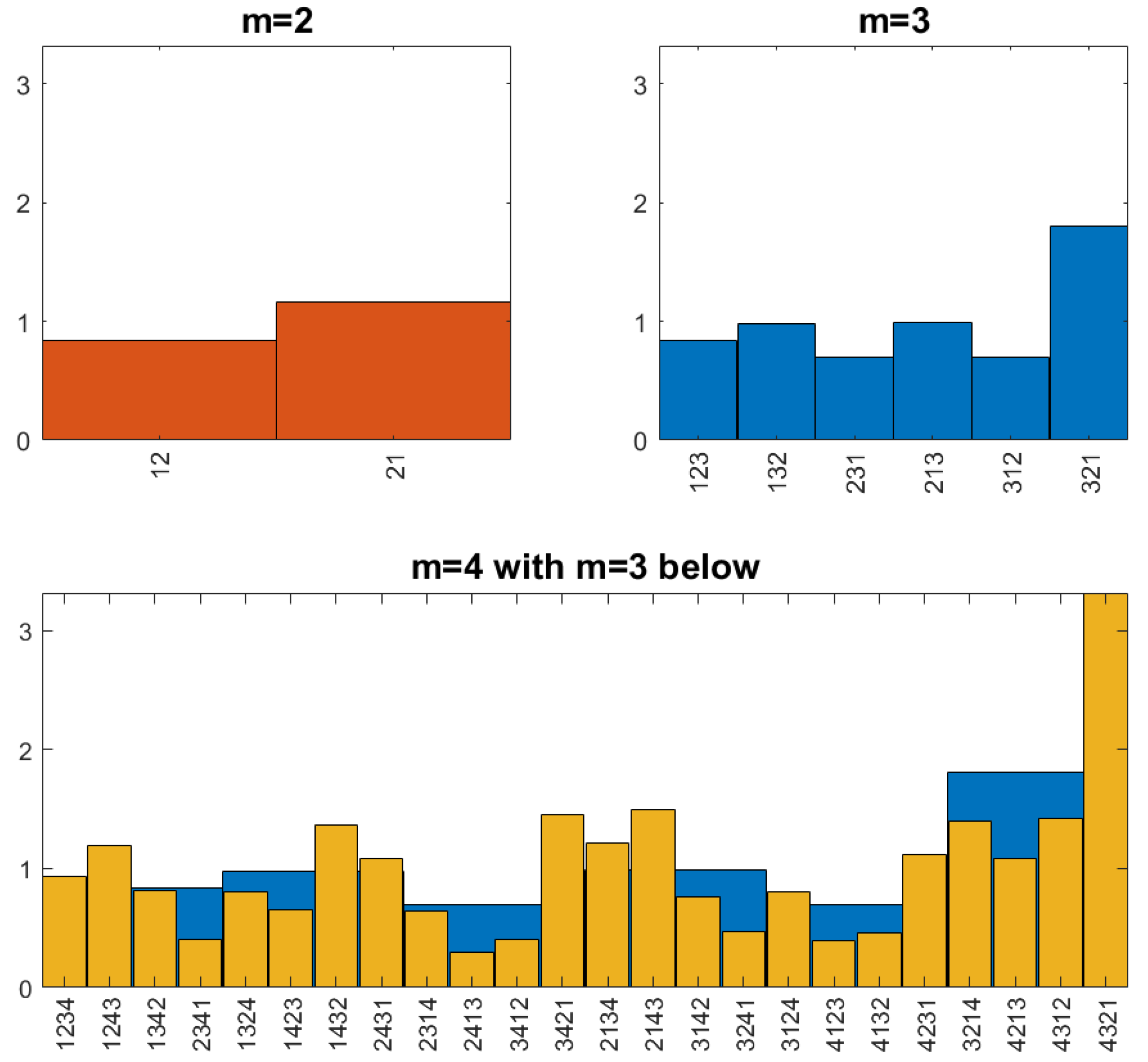
Figure 2.
Global and local rank numbers obtained from coin tossing.
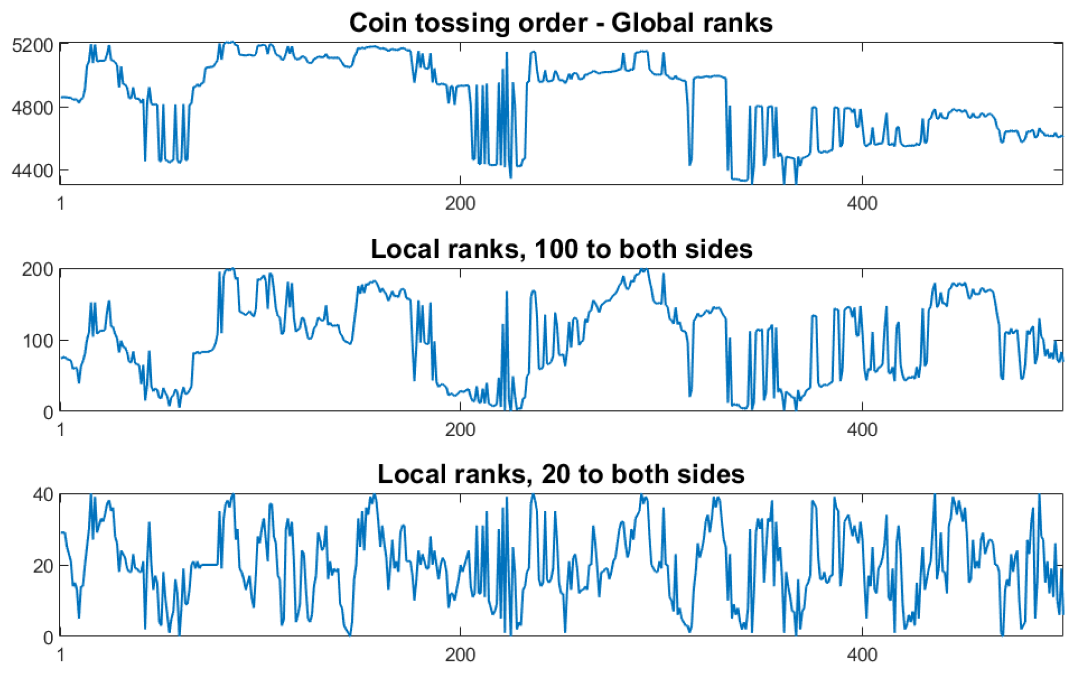
Figure 4.
Probabilities of patterns of length 4 for coin tossing order with and They are clearly different from while the changes from to are small.
Figure 4.
Probabilities of patterns of length 4 for coin tossing order with and They are clearly different from while the changes from to are small.
Disclaimer/Publisher’s Note: The statements, opinions and data contained in all publications are solely those of the individual author(s) and contributor(s) and not of MDPI and/or the editor(s). MDPI and/or the editor(s) disclaim responsibility for any injury to people or property resulting from any ideas, methods, instructions or products referred to in the content. |
© 2025 by the authors. Licensee MDPI, Basel, Switzerland. This article is an open access article distributed under the terms and conditions of the Creative Commons Attribution (CC BY) license (http://creativecommons.org/licenses/by/4.0/).
Copyright: This open access article is published under a Creative Commons CC BY 4.0 license, which permit the free download, distribution, and reuse, provided that the author and preprint are cited in any reuse.


