
Submitted:
06 May 2025
Posted:
08 May 2025
You are already at the latest version
Abstract
Determining the optimal controller settings in adaptive control systems for hydraulic drives is challenging. This is due to nonlinearities, parameter variability, and the influence of external disturbances. The proposed method assumes that varying operating conditions and control errors result in dynamic changes in system parameters. The controller parameters were adjustedvia the indirect identification of a linear model combined with the weighted recursive least squares (WRLS) method, ensuring continuous model adaptation to current operating conditions.The identification process included signal filtering using differentiating filters, which enabled precise derivative estimation in the presence of measurement noise, which is a key aspect of adaptive control. The applied filters allowed us to accurately determine system dynamics and improve parameter estimation accuracy. The experimental results confirmed that the application of adaptive control using the WRLS algorithm significantly enhances hydraulic system precision. In particular, in the system under study, the use of the WRLS method, with the additional adjustment of PD controller settings based on the control error, led to a satisfactory improvement in tracking error.
Keywords:
adaptive control systems
; hydraulic system
; WRLS
1. Introduction
Due to their ability to generate large forces and provide precise position and velocity control, hydraulic systems are widely used in the machinery, aerospace, and automotive industries. However, their dynamic properties, such as nonlinearity, parameter variability, and susceptibility to disturbances, pose challenges for classical control methods, such as PID controllers. As a result, there is growing interest in adaptive control, which allows the controller parameters to be adjusted to changing operating conditions.
Due to increasing demands for precision and reliability, modern hydraulic systems require more advanced control methods. A key factor is the controllers’ ability to adapt autonomously to changing operating conditions, which allows for maintaining optimal system performance without the need for manual control parameter adjustment. The use of adaptive control enables effective compensation for nonlinearity and model uncertainty, leading to more precise and stable regulation.
The dynamics of hydraulic systems are inherently nonlinear and influenced by various factors, such as variable fluid properties, flow–pressure relationships, and mechanical friction. These characteristics limit the effectiveness of classical control methods, which are typically based on simplified static models. As a result, maintaining consistent performance becomes difficult, especially under variable working conditions and external disturbances. This highlights the need for adaptive control approaches capable of real-time compensation and model updates.Effective compensation for undesired effects such as friction or valve nonlinearity is essential in hydraulic system control. Studies in the literature emphasize real-time parameter identification as a foundation for adaptive control strategies. These strategies enable the continuous refinement of the control law in response to changing system behaviour.
This study explores the potential of combining the WRLS algorithm with a tailored forgetting factor and adaptive PID controller gain tuning based on the absolute value of the control error. The goal is to enhance control precision and robustness. While initial results are promising, further experimental validation is needed to confirm the extent of improvement. Adaptive control allows for the real-time adjustment of controller parameters according to the current state of the system. Unlike classical approaches, such as PID or LQR, adaptive control does not require precise knowledge of the system model but instead employs algorithms that identify changing parameters in real-time. The most commonly used methods include the following:
- Model Reference Adaptive Control (MRAC)—the controller adjusts its parameters so that the system's response closely matches a reference model.
- Control with Parameter Estimation (RLS, WRLS)—the recursive parameter estimation method enables the identification of changing hydraulic systemproperties.
- Adaptive sliding mode control (Adaptive SMC)combines the advantages of robust sliding mode control with adaptive parameter regulation, enhancing the system's ability to suppress disturbances.
- Model Predictive Control (MPC)utilizes a mathematical model of the system to predict future states and optimize the control trajectory.
WRLS outperforms SMC and MRAC methods in many aspects, especially in applications requiring smooth adaptation to changing system conditions.
One of the key advantages of WRLS is its ability to adapt the model parameters in realtime, making it suitable for controllers based on system identification. Unlike MRAC, which requires a precisely defined reference model, WRLS can work effectively even when the initial model is poorly defined.
Additionally, WRLS eliminates chattering, a common issue in sliding mode control. This produces a smoother control signal, reducing unwanted oscillations and enhancing its applicability in systems requiring stable regulation.
Another advantage of WRLS is its easier interpretability and optimization potential compared to MRAC and SMC, which often require selecting numerous adaptive parameters or designing sliding surfaces. WRLS allows for the continuous updating of the system model, facilitating controller performance and tuning analysis.
In comparison to MRAC and SMC, WRLS also stands out for its superior ability to adapt to changing system properties. In hydraulic systems, where parameters can dynamically change (e.g., due to leaks or temperature variations), WRLS allows for smooth model adaptation, while MRAC and SMC often face limitations in adaptation, potentially leading to control instability (Table 1).
Studies in the literature highlight the widespread application of adaptive methods in hydraulics, examples of which include the following:
- Hydraulic actuator control;
- Automatic transmission control;
- The aerospace industry;
- Robotics.
Various approaches to adaptive control in hydraulic systems have been presented in the literature. Manring and Fales (2019) discussed the fundamental principles of hydraulic systems and classical control methods [1]. Li and Zhang (2022) proposed robust adaptive fuzzy control for electrohydraulic actuators, highlighting its advantages in compensating for parameter uncertainties [2]. Gu et al. (2018) developed an adaptive control system resistant to input constraints and valve dead zones, improving control precision [3]. Hampson (1995) introduced a nonlinear model of predictive control for hydraulic actuators, enabling the dynamic adjustment of the control strategy [4]. Cheng et al. (2019) focused on real-time sliding mode control for electrohydraulic power systems, proposing a new robust control method [5].
Zaare and Soltanpour (2022) applied optimal fuzzy backstepping control in electrohydraulic servo systems, improving system stability and robustness [6]. Zhong et al. (2024) utilized Model Reference Adaptive Control (MRAC) with radial basis function (RBF) neural networks and a disturbance observer, allowing dynamic control parameter regulation [7]. Deng et al. (2022) developed a neural network-based control strategy, achieving a better performance than classical control methods [8]. Wang et al. (2018) applied a fractional-order PID controller in hydraulic systems, enhancing system dynamics [9]. Guo et al. (2017) presented saturated adaptive control for electrohydraulic systems, demonstrating its effectiveness under variable parameters and disturbances [10].
Research highlights the broad potential of adaptive control in hydraulic systems. Kugi (2001) developed a physically based nonlinear control approach, improving hydraulic system precision [11]. Deng and Yao (2019) focused on using an extended state observer in the adaptive control of electrohydraulic servomechanisms, eliminating the need for velocity measurement [12]. Hao et al. (2021) introduced multi-criteria adaptive control for active hydraulic suspension, improving ride comfort and vehicle stability [13]. Guan and Pan (2008) applied adaptive sliding mode control in electrohydraulic systems, demonstrating its robustness against parameter uncertainties [14]. Gu et al. (2024) presented sliding mode control with adaptive compensation for drilling systems, enhancing control accuracy [15].
The cited publications show that many approaches, such as MRAC, SMC, MPC, and methods based on neural networks, have been studied in the literature [16]. Considering these works allows us to not only position WRLS in the context of other methods but also to highlight its unique advantages, such as lower computational complexity, greater flexibility, and better adaptability to changing operating conditions.
Further research explores modern approaches to adaptive control. Ellis (2012) described adaptive methods in control system design, integrating hydraulic control with other drive systems [17]. Rahbari and de Silva (2000) introduced fuzzy control in hydraulic systems, emphasizing its ability to adapt to changing operating conditions [18]. Vepa (2013) focused on hydraulic control in robotics, demonstrating its importance in autonomous systems [19]. Feng et al. (2019) applied the forgetting factor least squares algorithm for identifying hydraulic excavator models, improving their control [20].
The practical applications of adaptive control in hydraulic systems are also noteworthy. Klich and Kozieł (2010) developed a monograph on the design and operation of hydraulic systems, including adaptive aspects [21]. Dindorf et al. (2011) designed a real-time distributed control system for fluid servo drives using fuzzy logic [22]. Saków, Parus, and Miądlicki (2017) introduced a predictive force estimation method in feedback control for remotely operated hydraulic systems [23]. Pawelski (2010) discussed the adaptive control of oil pressure in automatic transmissions [24].
Ayinde and El-Ferik (2017) proposed adaptive backstepping control with an artificial bee colony algorithm for electrohydraulic servo systems with parameter uncertainties [25]. Pasolli and Ruderman (2020) presented an innovative approach to hybrid position and force control in hydraulic actuators, featuring autonomous mode switching [26].
Despite its many advantages, adaptive control presents the following challenges:
- High computational complexity, requiring control systems with significant processing power.
- Stability and convergence issues of adaptive algorithms in cases of sudden changes in operating conditions.
- Integration with modern machine learning methods, which can enhance the efficiency of adaptive control in hydraulics.
- Nonlinearities in hydraulic systems, which may complicate the design of control algorithms and require more advanced signal analysis methods.
The further development of adaptive control in hydraulic systems involves research on modern parameter estimation methods, such as hybrid algorithms based on Kalman filters and deep learning techniques. Advances in computational technology and increasing processor performance enable the implementation of more complex adaptive algorithms, opening up avenues for new industrial applications.
Adaptive control in hydraulic systems is a promising research direction that can significantly improve the precision and stability of these systems. Modern parameter identification methods, including the WRLS algorithm and adaptive sliding mode control, are increasingly applied in various industrial fields. The integration of adaptive methods with advanced signal processing techniques and artificial intelligence algorithms may be the next step in developing efficient hydraulic control systems.
The weighted recursive least squares (WRLS) method is one of the most popular real-time parameter identification algorithms, allowing for the adjustment of control strategies based on the system’s current state. The following sections will provide a detailed analysis of the WRLS algorithm, its implementation, and experimental results for a hydraulic system.
2. Identification Method
Identification methods are divided into on- and off-line approaches. The formerare used when the model must be known in realtime, such as in adaptive control. Off-line methods do not require immediate data processing.
In adaptive control systems, the model must adjust to changes in the object's parameters. To achieve this, parameter identification algorithms operate in parallel with measurements. Recursive identification algorithms allow real-time model updates.
One of the most popular algorithms is the least squares (LS) method; it is used for models with linear parameters (see Eq. (1)). The traditional LS algorithm operates off-line, meaning that all collected data are analyzed simultaneously. However, for systems with time-varying parameters, this method may be ineffective as it does not account for changes occurring over time.
This algorithm can be used for models with linear parameters, i.e.,
where
is a vector of unknown parameters,;
is a scalar signal,is a vector signal that is dependent, in a known way, on the measured signals (the plant input and output),
are the successive time instants.
The LS algorithm is based on the plant variables previously registered in a sufficiently long time interval . Measurement data are processed off-linebecause the identification process follows the measurement of the input and output variables.
To improve the algorithm's performance in dynamic conditions, a modification called the recursive least squares algorithm with exponential forgetting (WRLS) is used. In this method, older data have progressively less influence on parameter identification, allowing the model to better respond to real-time changes. The key element is the forgetting factor,, which controls how quickly older data lose significance (Eq.(2-4)).
The WRLS algorithm with exponential past data forgetting is obtained by minimizingthe objective function,
concerning the vector of the parameters,, where is a constant satisfying the inequality . Let represent a value of the vector of the parameters for which . Using a simple transformation, we obtain the following:
The forgetting factor choice depends on the system's rate of change and noise level. Values close to 1 result in slower data forgetting, which can improve identification stability but can also simultaneously reduce the ability to track sudden changes. A drawback of this method is that if no new data are available for an extended period, the values of matrices used in calculations may grow excessively, leading to system instability [27]. Research and simulations show that the value of this coefficient significantly affects the regulation outcome and parameter stability. The best results were obtained for the forgetting coefficient, , whichwas used in the study.
To avoid stability issues, parameter estimates are updated at specific sampling intervals. This approach allows for more accurate results, even in the presence of high noise levels.
Parameter estimates are updated after, a predefined number of signal sampling steps (). This assumption holds when the sampling period is relatively short compared to the expected rate of parameter variation. Additionally, a modification is introduced to ensure that the matrix remains bounded, regardless of whether the signal provides sufficient excitation(Eq.(5-7)).
Assuming that the plant equation follows the relationship inEq. (1), which depends on both the plant's input and output, a small sampling period typically results in insufficient information about the plant parameters within a single step. Therefore, it is considered that parameter estimates will be updated only after a predefined number of consecutive signal samples. The goal is to derive a recursive equation that determines the parameter estimates,, for time instances within the specified interval, .
Define the following objective function:
Generally, it is assumed that for in the range. Small initial values of the elements of the matrix ensure immediate convergence of the estimates to the real values of the parameters at the beginning of the algorithm.The initial parameter vector was assumed,, which represents a uniform initial assumption for all estimated model coefficients. This choice allows for a neutral starting point for the WRLS algorithm in the absence of prior knowledge about the true parameter values.
3. Tuning of PID Controller Settings
Modelling hydraulic systems is typically a challenging task due to their nonlinear nature, arising from the relationships between flow, pressure, and forces acting within the system. However, in many applications, it is possible to assume an approximated linear model (Eq.(8)) that effectively captures the key dynamic properties of the system. For this purpose, the transfer function is used:
This model describes a system consisting of an integrator coupled with a first-order inertial component and is particularly useful for position or velocity control systems. The properties of this model make it wellsuited for on-line identification methods, such as weighted recursive least squares (WRLS), enablingadaptive control parameter tuning in real-time.
Due to the asymmetric structure of the hydraulic actuator, it is assumed that for a control signal , the transfer function model will be considered, while for , the model will be used.
The main advantages of this modelling approach are as follows:
- Consideration of the integrating nature of the hydraulic actuator, which reflects the physical relationship between flow and piston displacement.
- Accounting for the asymmetric structure of the hydraulic actuator, which corresponds to the different dynamics of the system.
- Representation of control and damping dynamics through the time constant, , allowing the inclusion of effects resulting from inertia, viscosity, and oil compressibility.
- Ease of parameter identification based on experimental system responses.
- Suitability for adaptive control, where the parameters and can be updated in realtime to ensure optimal control performance.To compensate for system dynamics and ensure good control quality, a PID controller is applied with the following tuning parameters:
Proportional gain, which depends on the sum of the system's time constants and is scaled, is as follows:
The integral time constant determines the compensation dynamics of the control error and is equal to the sum of two characteristic time constants:
The derivative time constant is a function of the ratio of the system's response time to the sum of time constants, allowing for delay compensation and improving response dynamics:
where
is thetime constant of the system;
isan additional parameter related to the settling time.
This method allows for the automatic adjustment of settings based on the system's dynamics and the required regulation time. Since the model includes an integrator, proper tuning of the derivative component is necessary to avoid overshoots and oscillations. Parameter selection ensures a trade-off between response speed and system stability. The influence of regulation time on controller parameters should be considered in control optimization; higher values improve response speed but may cause greater oscillations, whereas lower values ensure stability at the cost of system dynamics.
For the analyzed system, when >5, the response exhibited significant overshooting and oscillations, causing instability. On the other hand, for <3, the hydraulic system exhibited poor dynamics. Therefore, a time constant range of 3≤≤5 was chosen. In the proposed algorithm, the value of changes depending on the absolute value of the error (Eq. (13)).
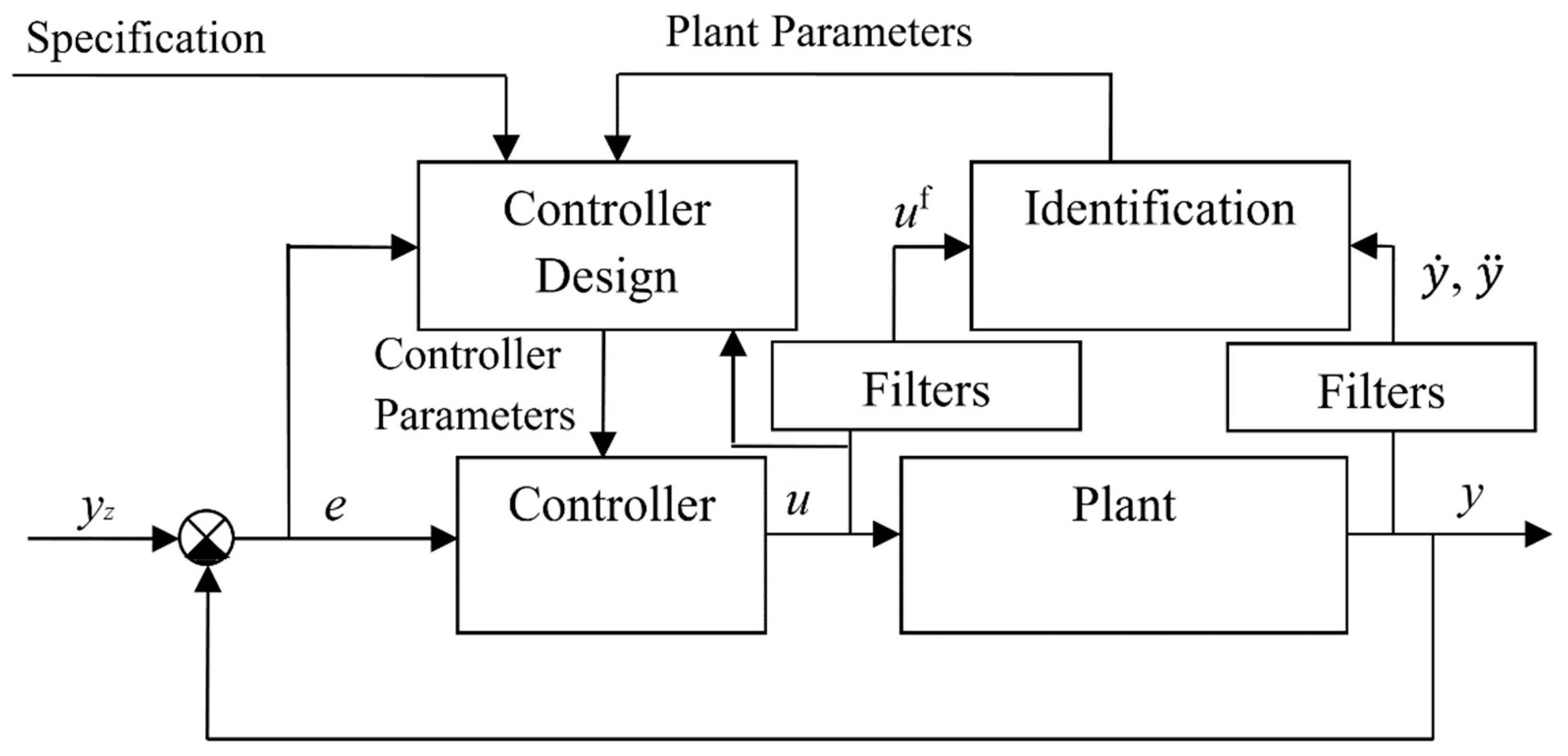
The adaptive control system is based on on-line identification using the WRLS method.
The controlled system is a system whose dynamics change over time. The output signal yy is measured and used for identification and control. The controller receives the error signal (the difference between the setpoint and the actual system output ). It generates the control signal based on the error and tuned parameters.
On-line identification uses the WRLS algorithm to estimate four system parameters () in realtime. It utilizes estimated signals for velocity and acceleration , which are obtained using appropriate differentiating filters. The identified system parameters are passed to the controller design module.
Differentiating filters process signals and to obtain the filtered signal and their derivatives (e.g.,,). The use of filters allows for more accurate derivative values while reducing the impact of measurement noise [28,29].
Controller designis performedand settings determined based on the identified system parameters and control error.
The presented system accounts for control specifications and the system's current characteristics. It transmits new parameter values to the controller for adaptive operation adjustment.
The advantages of using WRLS in adaptive control are as follows:
✔ Dynamic adaptation—the method allows for the real-time adjustment of controller settings to changing system properties.
✔ Noise reduction—the use of differentiating filters improves the quality of input signals for the identification algorithm.
✔ Improved estimation accuracy—thanks to the forgetting factor , the WRLS method responds more quickly to changes in system dynamics.
Figure 1.
Adaptive control system.
The tuning method automatically determines PID controller parameters based on system characteristics and the required regulation time, .
The following steps can be distinguished:
-Time requirement specification (the user defines the required regulation time,, depending on the error );
- Stability check ().
Controller parametersare calculated based on the stable model and time requirements.
Figure 2.
Adaptive control system (controller design).
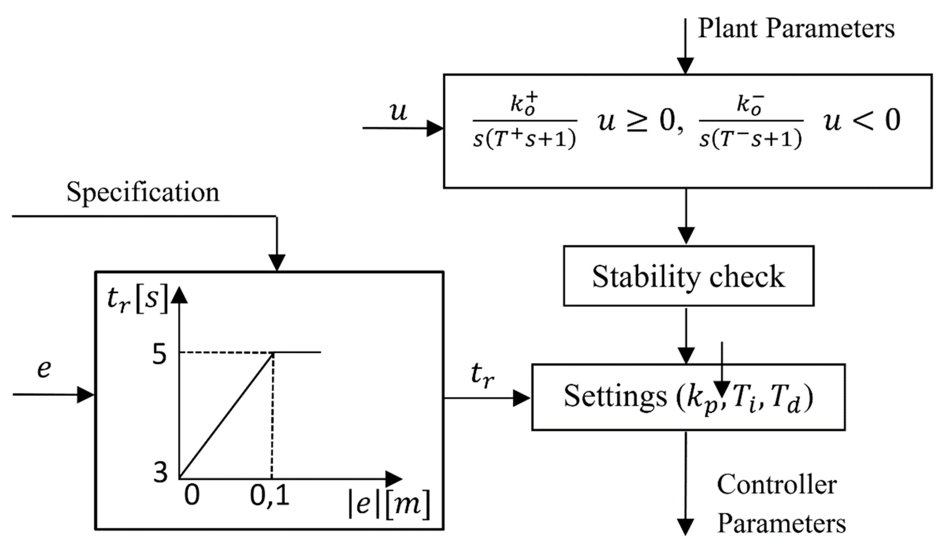
This method automates the PID controller tuning process, taking into account both dynamic requirements and the characteristics of the hydraulic model. The key stages include error analysis, modelling, stability verification, and final determination of PID controller settings. As a result, the system can be dynamically adjusted depending on operating conditions.
Due to the asymmetric structure of the hydraulic actuator, the dynamic properties of the system vary depending on the direction of motion. Therefore, two separate models are employed. The control algorithm continuously monitors the sign of the control signal and switches between the models accordingly. To ensure a smooth transition and avoid sudden changes in parameter estimation or controller action, a hysteresis threshold around is introduced. This prevents frequent switching between models caused by noise or small signal fluctuations.
Despite promising results, several limitations must be considered in the implementation:
Control loop frequency, data acquisition speed, and computational delays: In the presented system, the control loop operates at a frequency of 1 kHz, providing an adequate resolution for the hydraulic system's dynamics. The delay associated with signal filtering is 0.004 s.
The WRLS algorithm: Despite its low computational complexity making it suitable for real-time execution, it requires optimization, especially on platforms with limited computational resources.
Switching logic between models G⁺ and G⁻: This may lead to oscillations (chattering) or instability, particularly in the presence of noise or model uncertainties.
Impact of control loop frequency and delays: These factors directly affect the effectiveness of adaptive tuning and system stability.
4. Test Bench
The test bench was designed for testing and controlling hydraulic systems using modern technologies [30]. It consists of various components that enable the precise management of hydraulic fluid flow, pressure regulation, and system performance monitoring. Modern laser technologies were used to manufacture the structural elements [31,32,33]. The setup allows for hydraulic control system research and control algorithm testing. With the integration of advanced sensors and precise control elements, the test bench is suitable for both industrial and academic applications, supporting optimization and the development of modern hydraulic solutions.
A structural diagram of the test bench is illustrated in Figure 3. The hydraulic system consists of two HM0 60.35.0300 hydraulic cylinders, which serve as the primary components. The left-side cylinder functions as an actuator, while the right-side cylinder is used to simulate any external load (force). The cylinders are mounted in an opposing arrangement and interact with a force sensor with a measurement range of 0–17 kN.
The system is powered by a 4 kW hydraulic pump, generating an operating pressure of 18 MPa. Hydraulic oil flow control is managed using 4/4 NG 6 and 4/4 NG 10 directional control valves, which allow for flow direction changes and cylinder movement control. Additionally, proportional pressure valves WZPSE6 are used to regulate the hydraulic pressure required to simulate force on the right-side cylinder.
Pressure measurement is performed using PN3571 transducers. Data on the force generated by the actuators are recorded using a force sensor. The control and measurement system utilizes an NI PXI-6232 data acquisition card and an NI PXI-1031 (NI PXI-8110) real-time controller, along with a computer. Position measurement is handled by a PTx300 series linear displacement transducer connected to an MPL 104 amplifier. This system enables both data acquisition and test bench parametercontrol (Figure 4).
Each experiment was repeated twice to assess the repeatability of the results. The conditions in the laboratory setup varied between successive trials, and the oil temperature, which changed from 25°C to 60°C over 15 minutes of operation, had an impact on the results. Despite these changing conditions, the obtained results were very similar, indicating the stability of the experiments.
To confirm the reliability of the results obtained from the research setup, five trials were conducted with an adaptive PD controller. Based on the obtained results, the quality of the data and the stability of the experiment were evaluated:
The mean MAE of 0.02210004 suggests that the model adequately represents the data. This value falls within the expected range, indicating a low absolute error.
The standard deviation of 0.00014357 is very small, indicating low variability in the results. This means the results are relatively stable, and the measurement error does not introduce significant fluctuations.
The 95% confidence interval, 0.02210004 ± 0.00017826, is very narrow, suggesting that the estimation of the mean MAE is precise and reliable. There is 95% confidence that the true mean MAE falls within this range. The narrow width of the interval underscores the stability of the results.
The coefficient of variation (CV) of 0.6496% is very low, indicating minimal variability relative to the mean. This result demonstrates the high precision of the measurements.
The t-Student test: p = 0.000000000427391 indicates that the test result is different from zero. The p-value is significantly smaller than 0.05, confirming that there is a statistical difference between the means. This means the experimental results are not random, and there is a statistically significant difference in the means.
The obtained results are very stable and reliable, and the data exhibit high precision. The low variability of the results (low coefficient of variation and narrow confidence interval) indicates strong consistency in the experiment. The result of the t-Student test suggests that the means differ significantly, which is expected when there are meaningful differences in the measurements. In summary, the data are well consolidated, and the experiment provides reliable and precise results.
5. Obtained Results
This chapter presents the experimental results, evaluating the quality of adaptive control in a hydraulic system. A control system comparison was conducted for both off- and on-line models with constant and variable values of .The comparative study of the hydraulic system began with the off-line identification of a linear system model. In the proposed method, tuning the PID controller requires model knowledge, which is defined in the form of a transfer function. In this case, the input signal is the voltage uu that controls the amplifier of the proportional valve, while the output signal represents the piston position of the actuator.
The parametric identification problem of the linear mathematical model of the electrohydraulic system involves determining the unknown parameters of the transfer function or based on measurements of the control signal and the piston position . For the maximum input signals and , the transfer function parameters were determined (Figure 5 and Figure 6).
For off-line identification, the classical output error method was applied using the optimization function lsqnonlin. By minimizing the integral squared error (ISE) for the analyzed hydraulic system, the following parameters were obtained.
A linear mathematical model with constant parameters describes the system dynamics fairly well at a constant velocity. However, real phenomena occurring during actuator movement are nonlinear due to factors such as dry and viscous friction.
The following charts (Figure 7, Figure 8, Figure 9, Figure 10 and Figure 11) present the results obtained for the PD controller with a variable value of (online) and a model identified in realtime (online), as well as for the PD controller with fixed parameters.The fixed settings were determined based on off-line models and a time constant of Figure 7 illustrates the variations in the control voltage applied to the proportional valve amplifier. This signal appropriately excites the system, enabling accurate parameter identification and analysis of the object's dynamics.
The system response and reference signal in Figure 8 allow us to assess how well the control system tracks the desired trajectory.
During the control process, changes in the controller parameters, hydraulic fluid pressure, and regulation time dependent on the error were recorded.
Figure 9 presents the proportional gain value of the controller. The dynamic change in this value illustrates how the adaptive system modifies the settings to better adjust to the current operating conditions of the system.
Figure 10 shows the variations in the integral time constant . This parameter influences the elimination of the steady-state error; its adaptive adjustment helps in faster error correction, resulting from differences between the setpoint and the actual value.
Figure 11 illustrates the variations in the derivative time constant, which is responsible for damping oscillations and improving response dynamics. The changing value demonstrates how the adaptive system reacts to sudden changes, reducing overshoot.
Figure 12 presents the regulation time, a parameter influencing controller setting calculations. According to the adopted assumptions, its value can vary between 3 and 5, with the maximum change occurring when the error is =0.1 [m]. The parameter range and its variation method were selected experimentally to ensure stable system operation and optimal control performance.
The direct excitation is the active force acting on the piston (Eq.(14)); this is calculated based on the recorded pressures (Figure 13). This chart illustrates the system's operation under variable conditions, making it suitable for adaptive control applications.
where
are the piston surfaces(0.002828 [],0.001864[]);
are pressures.
Table 2 summarizes the control results for different configurations, comparing control using PID, PD, and P controllers with both on- and off-line models. The presented MAE (mean absolute error) values indicate that the adaptive approach based on on-line identification generally yields slightly better results (lower MAE), confirming the effectiveness of dynamic tuning. Applyingthe developed control method improves trajectory tracking and control quality. The tracking error values significantly improve when an on-line identified model is used. The best results were achieved with the PD controller featuring variable regulation time and an on-line identified model.
For the PID controller, the on-line configurations demonstrate a significantly greater improvement in response time compared to the off-line settings, achieving reductions of up to approximately 17.3%. The PD controller also shows enhanced performance in the on-line configurations, with response time improvements reaching 18.1%, although the differences are slightly smaller than those observed for the PID controller. In the case of the P controller, the differences between on- and off-line configurations are less pronounced, with a maximum improvement of about 15.0%. These results indicate a consistent and substantial enhancement in the control system’s dynamic performance, particularly for the PID and PD controllers operating in on-line configurations (Table 3).
Statistical significance testing (t-test) confirmed that each of the evaluated configurations (on-line/on-line, on-line/off-line, 3/on-line) yielded a statistically significantly lower mean absolute error compared to the baseline configuration (3/off-line). The observed p-values (p < 0.001), along with strictly positive 95% confidence intervals for the MAE differences (approximately 1.6 mm to 7.8 mm), support both the statistical significance and the practical relevance of the observed improvements (Table 4).
Interpreting the mean absolute error differences (ΔMAE) reveals the following:
- A ΔMAE of 0.007 metres corresponds to an error of approximately 7 mm in positioning. Depending on the specific system, such an improvement could represent a significant enhancement in precision and overall system performance.
- All observed ΔMAE values fall within the range of approximately 0.002 to 0.007 metres. For systems requiring precision at the millimetre scale, these differences are of considerable practical significance, underscoring the effectiveness of the improvements in real-world applications.
In the weighted recursive least squares method, the forgetting factor plays a crucial role in estimating model parameters. Its value determines how quickly the algorithm "forgets" past observations, enabling better change tracking in dynamic systems. Various forgetting factor values and their impact on control performance were analyzed (Table 5 and Table 9).
Selection of value:
• = 1 corresponds to the classical recursive least squares method without forgetting, where all data points have equal weight.
• < 1 introduces a forgetting mechanism in which newer observations have a greater influence on parameter estimation than older ones. The smaller the value of , the faster the forgetting and the greater the adaptability of the algorithm.
Table 6 analyzes the different numbers of points and their impact on regulation quality.
In Table 7, an analysis of the parameters depending on is presented, including the standard deviation and 95% confidence intervals.
• Higher values of lead to higher values of and , while reducing the confidence interval, resulting in a more stable estimation.
• The parameter remains independent of , indicating its resistance to the influence of the forgetting factor.
• Smaller confidence intervals for higher indicate greater confidence in the results.
The most stable values are obtained for ≈0.95−0.99. The range of ≈0.97−0.99 provides the highest precision and result stability, while a faster response to changes in the system can be achieved for ≈0.89−0.91.
Simulation model studies were also conducted based on transfer functions identified off-line. The results of these studies confirmed that the optimal value of the forgetting factor is 0.89, and the best choice is points. For these parameters, the smallest MAE index was obtained, indicating their effectiveness in improving control accuracy (Table 8, Table 9 and Table 10).

Table 8.
Control simulation results.
| Controller | [s] | Model | MAE [m] | Tracking error improvement[%] |
| PID | on-line | on-line | 0.00724004 | 28.5 |
| on-line | off-line | 0.00860414 | 15.1 | |
| 3 | off-line | 0.01013450 | 0.0 | |
| 3 | on-line | 0.00811677 | 19.9 | |
| PD | on-line | on-line | 0.00723945 | 28.5 |
| on-line | off-line | 0.00860297 | 15.1 | |
| 3 | off-line | 0.01013370 | 0.0 | |
| 3 | on-line | 0.00811597 | 19.9 | |
| P | on-line | on-line | 0.00750426 | 10.0 |
| on-line | off-line | 0.00746252 | 10.5 | |
| 3 | off-line | 0.00833968 | 0.0 | |
| 3 | on-line | 0.00776261 | 6.9 |
Table 9.
Simulation results of control (N = 500).
| Controller | MAE [m] | |
| PD | 0.86 | 0.00744240 |
| 0.88 | 0.00747660 | |
| 0.89 | 0.00723945 | |
| 0.90 | 0.00727522 | |
| 0.91 | 0.00731916 | |
| 0.95 | 0.00777959 | |
| 0.97 | 0.00810926 | |
| 0.99 | 0.00831892 |
Table 10.
Simulation results of control (λ = 0.89).
| Controller | MAE [m] | |
| PD | 100 | 0.00804101 |
| 200 | 0.00785074 | |
| 300 | 0.00777552 | |
| 400 | 0.00797071 | |
| 500 | 0.00752388 | |
| 600 | 0.00765852 | |
| 800 | 0.00781735 | |
| 1000 | 0.00833439 |
The analysis conducted revealed significant differences between the control methods. The results of statistical tests confirm that the application of the WRLS method leads to a significant improvement in control accuracy. The obtained results indicate the potential application of the WRLS method in real hydraulic systems, particularly where adaptive control is required for changing operating conditions. The implementation of this method can improve the stability and precision of control in industrial applications, such as hydraulic actuator control in construction machinery and industrial robots.
The experimental results show that the mathematical model obtained using the off-line method accurately represents the system dynamics under steady conditions. However, under varying conditions (and in the presence of nonlinearities) discrepancies may occur. The dynamic adaptation of controller parameters (changes in gain, integration, and differentiation constants) enables better control adjustment to current conditions, positively impacting the setpoint tracking quality. The MAE analysis in the table confirms that configurations based on the on-line model result in lower control errors, which is crucial for achieving precise control tasks in hydraulic systems.
6. Conclusions
The experimental results conducted on the hydraulic system confirm that the application of adaptive PID control with automatic parameter adjustment improves control quality. The use of the WRLS algorithm reduced the mean tracking error by 24.4%, while optimizing the forgetting factor within the 0.86−0.99 range ensured system stability. A statistical analysis of the estimated model parameters showed a standard deviation below 0.001321, confirming the reliability of the identification process.
Furthermore, this study aligns with the findings presented in [29], the authors of which analyzed the effectiveness of differentiating filters in mitigating quantization noise in 16-bit converters. In this work, similar 16-bit converters were used, and the applied filters effectively reduced high-frequency disturbances, minimizing the impact of measurement noise on the control process.The use of low-pass and differentiating filters contributed to achieving high-quality control. In the discussed hydraulic system, a key role was played by the identification procedure based on the WRLS algorithm, which allowed for the accurate estimation of mathematical model parameters, enabling the optimal tuning of the controller settings.
Thanks to the real-time automatic adjustment of controller gains, the system effectively compensated for nonlinearities arising from phenomena such as friction or variable properties of the working fluid, resulting in stable operation and improved tracking performance. Unlike classical PID controllers with fixed settings, the adaptive control system responds in realtime to changing operating conditions, ultimately reducing control error and increasing disturbance resistance [34,35,36,37,38].
A crucial aspect of the applied method is the use of differentiating filters, which enabled the precise determination of signal derivatives despite a high level of measurement noise. The filter design process minimized estimation errors, directly influencing the accuracy of parameter identification and the effectiveness of the WRLS algorithm.
The advanced adaptive system, based on automatic gain adjustment, exhibits significantly better control properties than traditional PID controllers. The adaptation procedure effectively handles system nonlinearities and dynamic changes in operating conditions, improving the precision of setpoint tracking. The proposed approach is versatile and has been successfully tested both in simulations and on a physical test bench with a step reference signal.
The presented results highlight the great potential of applying adaptive control methods in hydraulic systems, where dynamic parameter identification and automatic controller tuning can significantly enhance system precision and stability.
The main novelty of this study lies in the development and experimental validation of an adaptive control method for a hydraulic actuator using a forgetting-factor least squares estimator and differentiating filters.
Unlike conventional approaches that rely on fixed PID gains or a single model-based characteristic, the proposed method employs two linear models to capture the asymmetric behaviour of the actuator (resulting from the difference in piston areas on both sides) and an adaptive mechanism for tuning the controller gains based on the absolute value of the tracking error. The main contributions of the work include the following:
- The use of differentiating filters to improve parameter estimation quality under noisy conditions;
- The design of an adaptive PID control structure with gain selection based on the current model and error magnitude;
- The experimental verification of the proposed approach on a real test rig under varying load conditions.
Author Contributions
L.C.: conceptualization, methodology, supervision, project administration, validation, software, visualization, and writing—original draft; P.W.: writing—review and editing, data curation, visualization, and validation. All authors have read and agreed to the published version of the manuscript.
Funding
This research received no external funding.
Conflicts of Interest
The authors declare no conflicts of interest.
References
- Manring, N.D.; Fales, R.C. Hydraulic Control Systems; John Wiley & Sons: Hoboken, NJ, USA, 2019. [Google Scholar]
- Li, M.; Zhang, Q. Adaptive Robust Fuzzy Impedance Control of an Electro-Hydraulic Actuator. Appl. Sci. 2022, 12, 9575. [Google Scholar] [CrossRef]
- Gu, W.; Yao, J.; Yao, Z.; Zheng, J. Robust Adaptive Control of Hydraulic System with Input Saturation and Valve Dead-Zone. IEEE Access 2018, 6, 53521–53532. [Google Scholar] [CrossRef]
- Hampson, S.P. Nonlinear Model Predictive Control of a Hydraulic Actuator. University of Canterbury 1995.
- Cheng, L.; Zhu, Z.C.; Shen, G.; Wang, S.; Li, X.; Tang, Y. Real-Time Force Tracking Control of an Electro-Hydraulic System Using a Novel Robust Adaptive Sliding Mode Controller. IEEE Access 2019, 8, 13315–13328. [Google Scholar] [CrossRef]
- Zaare, S.; Soltanpour, M.R. Optimal Robust Adaptive Fuzzy Backstepping Control of Electro-Hydraulic Servo Position System. Trans. Inst. Meas. Control 2022, 44, 1247–1262. [Google Scholar] [CrossRef]
- Zhong, H.; Liu, K.; Qiang, H.; Yang, J.; Kang, S. Model Reference Adaptive Control of Electro-Hydraulic Servo System Based on RBF Neural Network and Nonlinear Disturbance Observer. Proc. Inst. Mech. Eng. Part I J. Syst. Control Eng. 2024. [CrossRef]
- Deng, W.; Zhou, H.; Zhou, J.; Yao, J. Neural Network-Based Adaptive Asymptotic Prescribed Performance Tracking Control of Hydraulic Manipulators. IEEE Trans. Syst. Man Cybern. Syst. 2022, 53, 285–295. [Google Scholar] [CrossRef]
- Wang, N.; Wang, J.; Li, Z.; Tang, X.; Hou, D. Fractional-Order PID Control Strategy on Hydraulic-Loading System of Typical Electromechanical Platform. Sensors 2018, 18, 3024. [Google Scholar] [CrossRef]
- Guo, Q.; Yin, J.; Yu, T.; Jiang, D. Saturated Adaptive Control of an Electrohydraulic Actuator with Parametric Uncertainty and Load Disturbance. IEEE Trans. Ind. Electron. 2017, 64, 7930–7941. [Google Scholar] [CrossRef]
- Kugi, A. Non-Linear Control Based on Physical Models: Electrical, Mechanical and Hydraulic Systems; Springer: London, UK, 2001. [Google Scholar]
- Deng, W.; Yao, J. Extended-State-Observer-Based Adaptive Control of Electrohydraulic Servomechanisms without Velocity Measurement. IEEE/ASME Trans. Mechatron. 2019, 25, 1151–1161. [Google Scholar] [CrossRef]
- Hao, R.; Wang, H.; Liu, S. Multi-Objective Command Filtered Adaptive Control for Nonlinear Hydraulic Active Suspension Systems. Nonlinear Dyn. 2021, 105, 1559–1579. [Google Scholar] [CrossRef]
- Guan, C.; Pan, S. Adaptive Sliding Mode Control of Electro-Hydraulic System with Nonlinear Unknown Parameters. Control Eng. Pract. 2008, 16, 1275–1284. [Google Scholar] [CrossRef]
- Gu, J.; Wang, X.; Yan, H.; Tan, C.; Si, L.; Wang, Z. Observer-Based Adaptive Sliding Mode Compensation Position-Tracking Control for Drilling Tool Attitude Adjustment. Sensors 2024, 24, 2404. [Google Scholar] [CrossRef]
- Zhang, D.Y.; Liu, S.Y.; Chen, Y.; et al. Neural Direct Adaptive Active Disturbance Rejection Controller for Electro-hydraulic Servo System. Int. J. Control Autom. Syst. 2022, 20, 2402–2412. [Google Scholar] [CrossRef]
- Ellis, G. Control System Design Guide: Using Your Computer to Understand and Diagnose Feedback Controllers; Butterworth-Heinemann: 2012.
- Rahbari, R.; de Silva, C.W. Fuzzy Logic Control of a Hydraulic System. Proceedings of IEEE International Conference on Industrial Technology 2000 (IEEE Cat. No. 00TH8482); IEEE, 2000; Volume 2, pp. 313–318. [Google Scholar]
- Vepa, R. Dynamic Modeling, Simulation and Control of Energy Generation; Volume 20; Springer: London, 2013. [Google Scholar]
- Feng, H.; Yin, C.; Yu, H.; Cao, D. Robotic Excavator Identification Model Based on Recursive Least Squares Algorithm with Forgetting Factor. In 2019 International Conference on Advances in Construction Machinery and Vehicle Engineering (ICACMVE); IEEE: 2019; pp. 352–356.
- Klich, A.; Kozieł, A. Badanie, Konstrukcja, Wytwarzanie i EksploatacjaUkładówHydraulicznych; Monografia, ISBN 978-83-60708-88-0; Wydawca: InstytutTechnikiGórniczej KOMAG.
- Dindorf, R.; Łaski, P.; Takoshoglu, J.; Woś, P. Rozproszony System SterowaniaCzasuRzeczywistego do SerwonapędówPłynowych. CzasopismoTechniczne. Mechanika 2011, 108, 43–48. [Google Scholar]
- Saków, M.; Parus, A.; Miądlicki, K. PredykcyjnaMetodaWyznaczaniaSiły w SiłowymSprzężeniuZwrotnym w SystemieZdalnieSterowanym. Modelowanie Inżynierskie 2017, 31, 88–97. [Google Scholar]
- Pawelski, Z. SkrzynieAutomatyczne: PodstawyDziałania; Monografia, Łódź, 2010; ISBN 978-83-7283-365-5.
- Ayinde, B.O.; El-Ferik, S. Artificial Bee Colony-Based Adaptive Position Control of Electrohydraulic Servo Systems with Parameter Uncertainty. arXiv 2017. [Google Scholar]
- Pasolli, P.; Ruderman, M. Hybrid Position/Force Control for Hydraulic Actuators. In 2020 28th Mediterranean Conference on Control and Automation (MED); IEEE: 2020; pp. 73–78.
- Zaborski, M. , Mańdziuk, J. Surrogate-Assisted LSHADE Algorithm Utilizing Recursive Least Squares Filter. In: Rudolph, G., Kononova, A.V., Aguirre, H., Kerschke, P., Ochoa, G., Tušar, T. (eds) Parallel Problem Solving from Nature – PPSN XVII. PPSN 2022. Lecture Notes in Computer Science, vol 13398. Springer, Cham.
- Cedro, L.; Janecki, D. Determining of Signal Derivatives in Identification Problems - FIR Differential Filters. Acta MontanisticaSlovaca 2011, 16, 47–54 ISSN 1335. [Google Scholar]
- Cedro, L. Filtryróżniczkujące w układachczasurzeczywistego. Przegląd Elektrotechniczny 2013, 89, 137–141 ISSN 0033. [Google Scholar]
- Szcześniak, A.; Szcześniak, Z. Algorithmic Method for the Design of Sequential Circuits with the Use of Logic Elements. Appl. Sci. 2021, 11, 11100. [Google Scholar] [CrossRef]
- Widłaszewski, J.; Nowak, Z.; Kurp, P. Effect of Pre-Stress on Laser-Induced Thermoplastic Deformation of Inconel 718 Beams. Materials 2021, 14, 1–18. [Google Scholar] [CrossRef] [PubMed]
- Kurp, P. Mechanically-Assisted Laser Forming of Flat Thin Beams Made of Inconel 627 and Inconel 718 Alloys. Materials Res. Proc. 2018, 5, 25–30. [Google Scholar]
- Kurp, P.; Danielewski, H. Metal Expansion Joints Manufacturing by a Mechanically Assisted Laser Forming Hybrid Method – Concept. Techn. Trans. 2022, 119. [Google Scholar] [CrossRef]
- Wang, X.; Yan, X.; Li, D.; Sun, L. An Approach for Setting Parameters for Two-Degree-of-Freedom PID Controllers. Algorithms 2018, 11, 48. [Google Scholar] [CrossRef]
- Dalen, C.; Di Ruscio, D. Performance Optimal PI Controller Tuning Based on Integrating Plus Time Delay Models. Algorithms 2018, 11, 86. [Google Scholar] [CrossRef]
- Kofinas, P.; Dounis, A.I. Fuzzy Q-Learning Agent for Online Tuning of PID Controller for DC Motor Speed Control. Algorithms 2018, 11, 148. [Google Scholar] [CrossRef]
- Almabrok, A.; Psarakis, M.; Dounis, A. Fast Tuning of the PID Controller in an HVAC System Using the Big Bang–Big Crunch Algorithm and FPGA Technology. Algorithms 2018, 11, 146. [Google Scholar] [CrossRef]
- Ju, J.; Zhao, Y.; Zhang, C.; Liu, Y. Vibration Suppression of a Flexible-Joint Robot Based on Parameter Identification and Fuzzy PID Control. Algorithms 2018, 11, 189. [Google Scholar] [CrossRef]
Figure 3.
Test bench diagram.

Figure 4.
Test bench view:1—hydraulic power supply,2, 3—hydraulic actuators,4—proportional valve 4/4 NG 6,5—proportional valve4/4 NG 10,6—pressure control valvesWZPSE6,7—force sensor,8—pressure sensor PN3571,9—displacement sensor, peltron PTx300.
Figure 4.
Test bench view:1—hydraulic power supply,2, 3—hydraulic actuators,4—proportional valve 4/4 NG 6,5—proportional valve4/4 NG 10,6—pressure control valvesWZPSE6,7—force sensor,8—pressure sensor PN3571,9—displacement sensor, peltron PTx300.
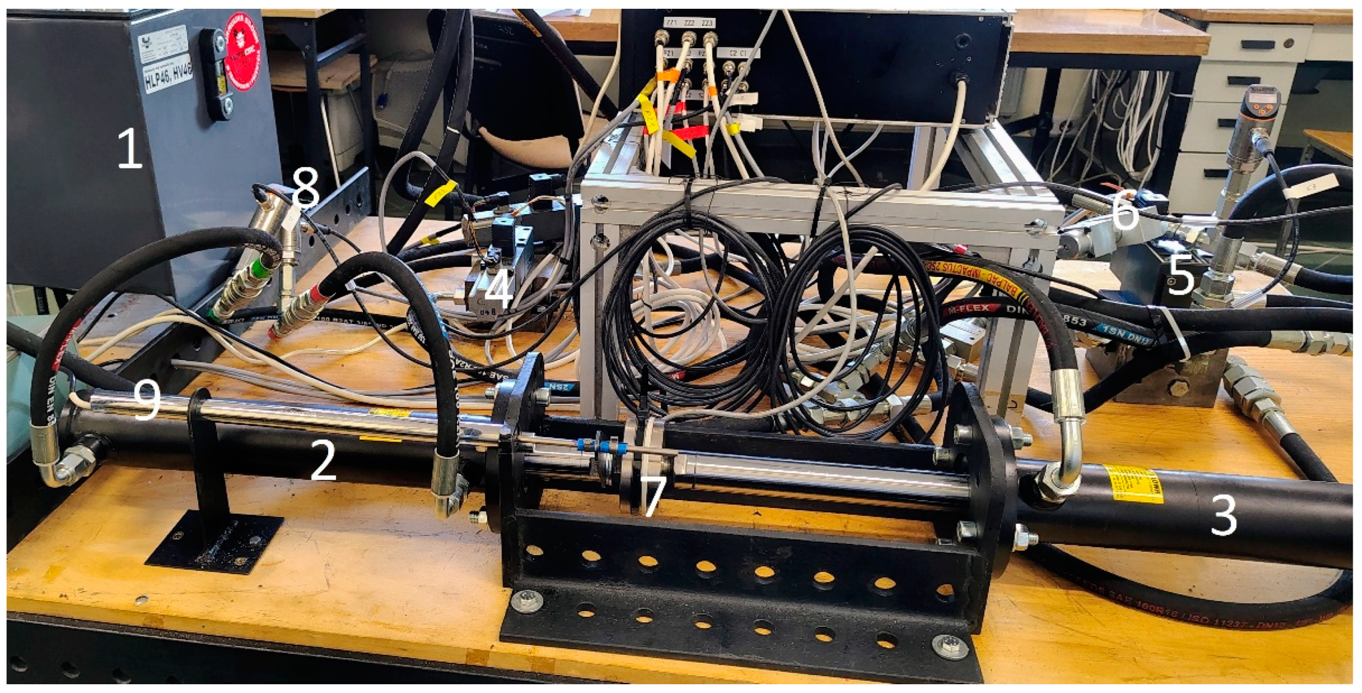
Figure 5.
Hydraulic system response and identified model for.
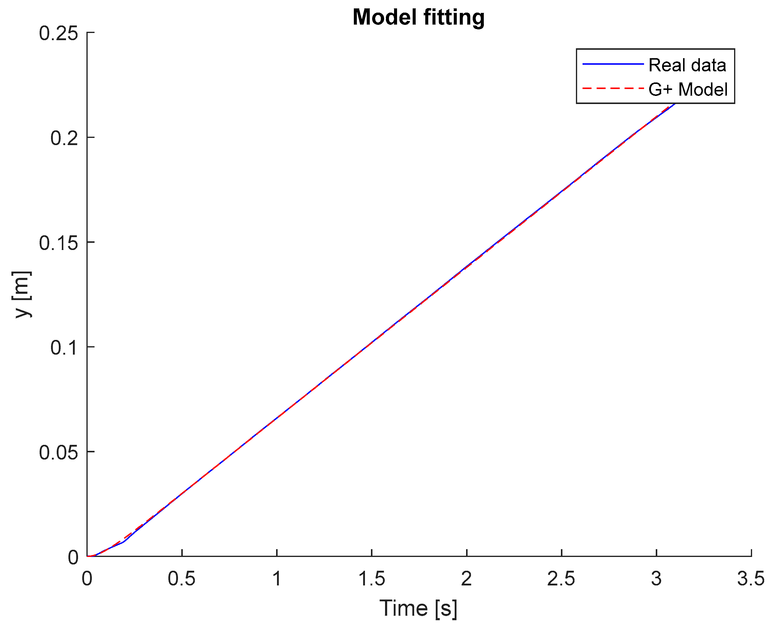
Figure 6.
Hydraulic system response and identified model for.
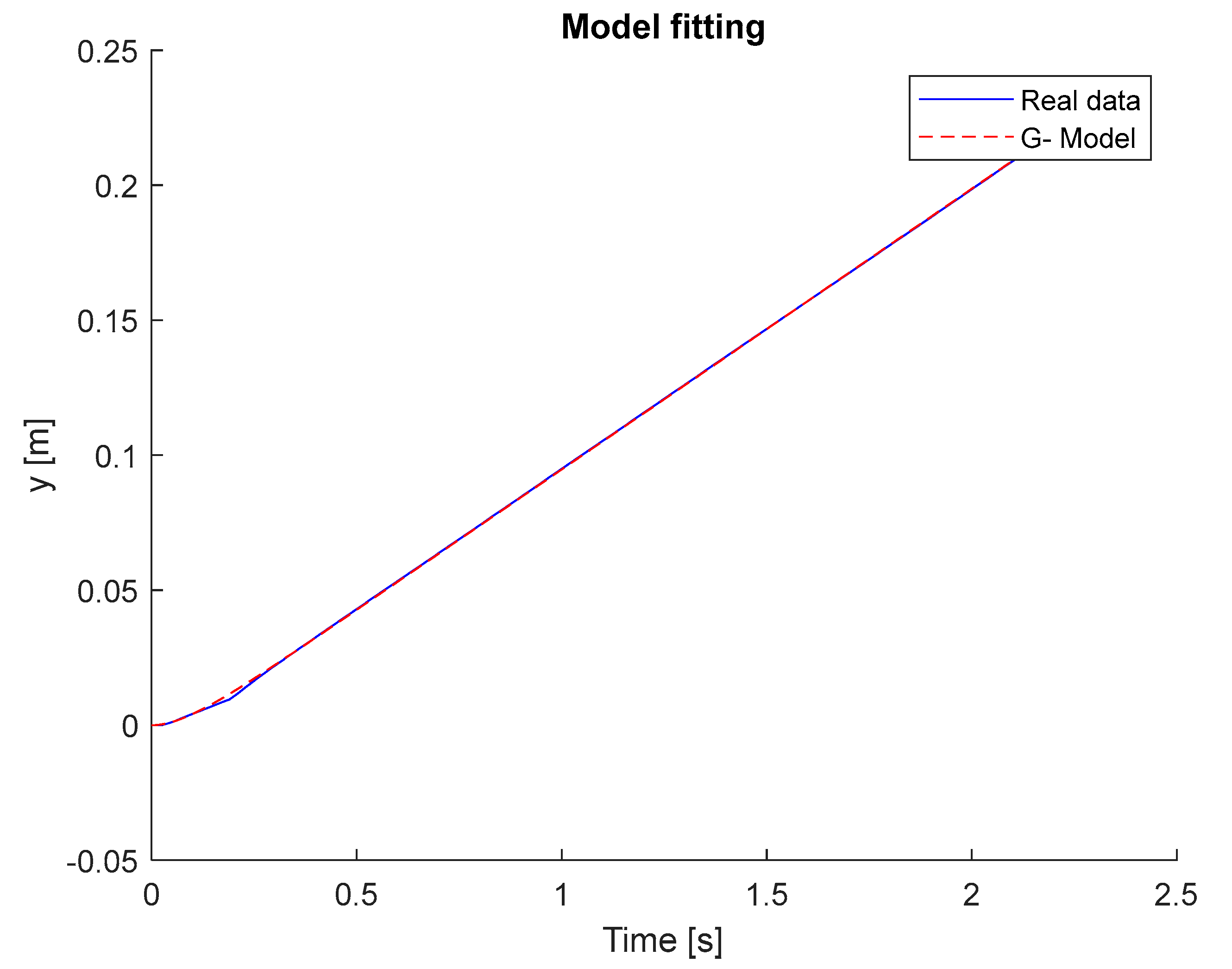
Figure 7.
System input signal.
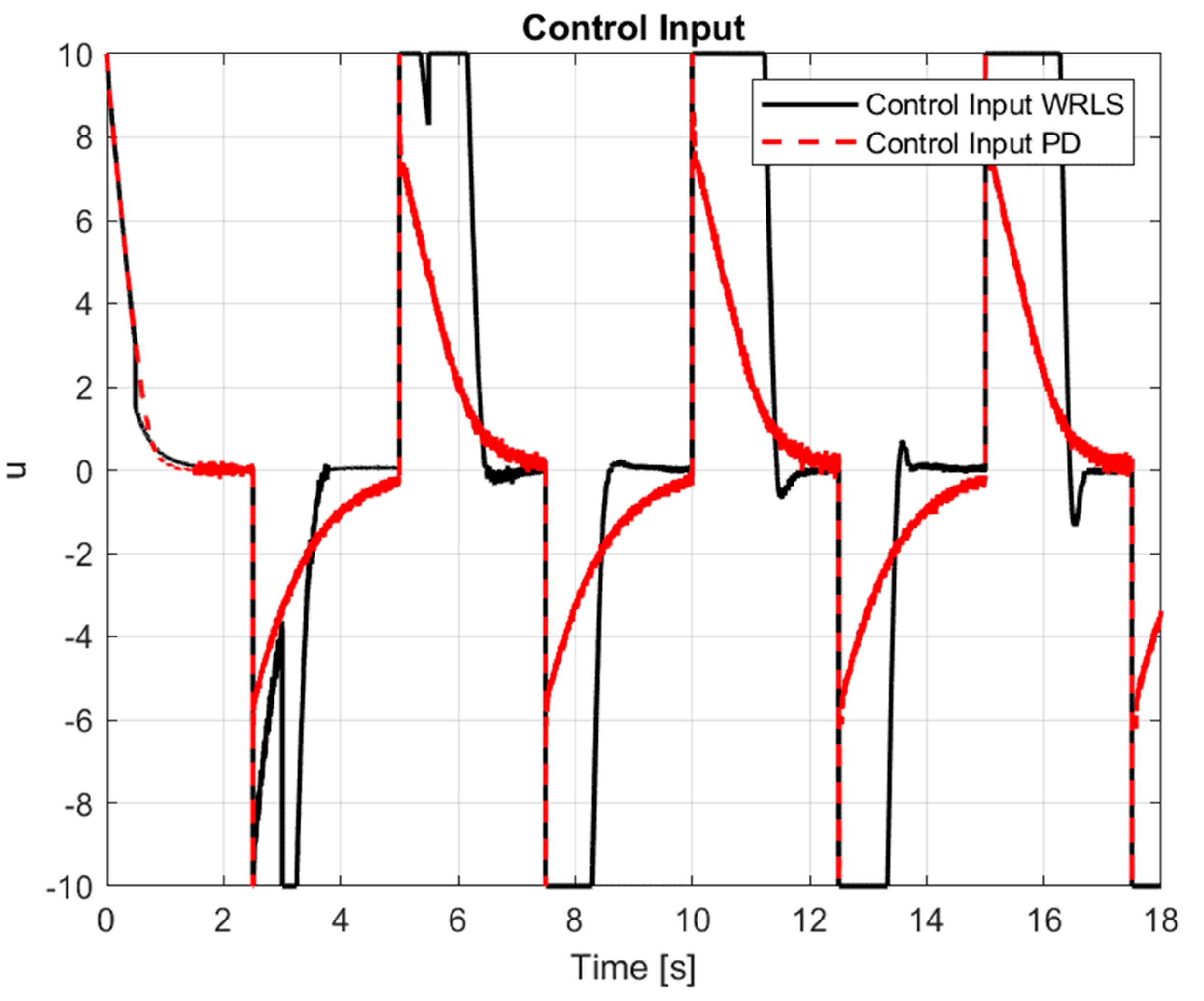
Figure 8.
System response and reference signal.

Figure 9.
Proportional gain .
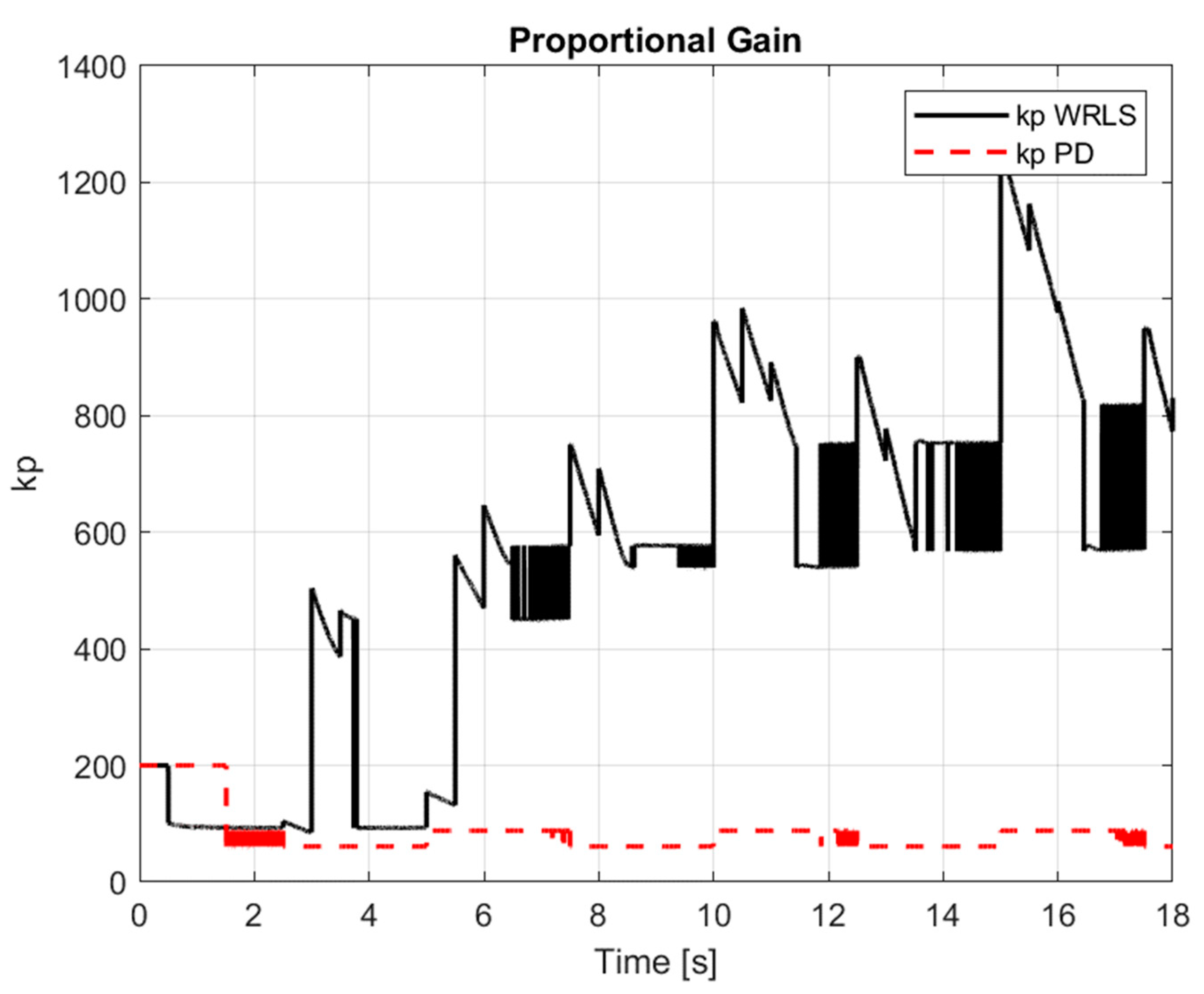
Figure 10.
Integral time constants, .
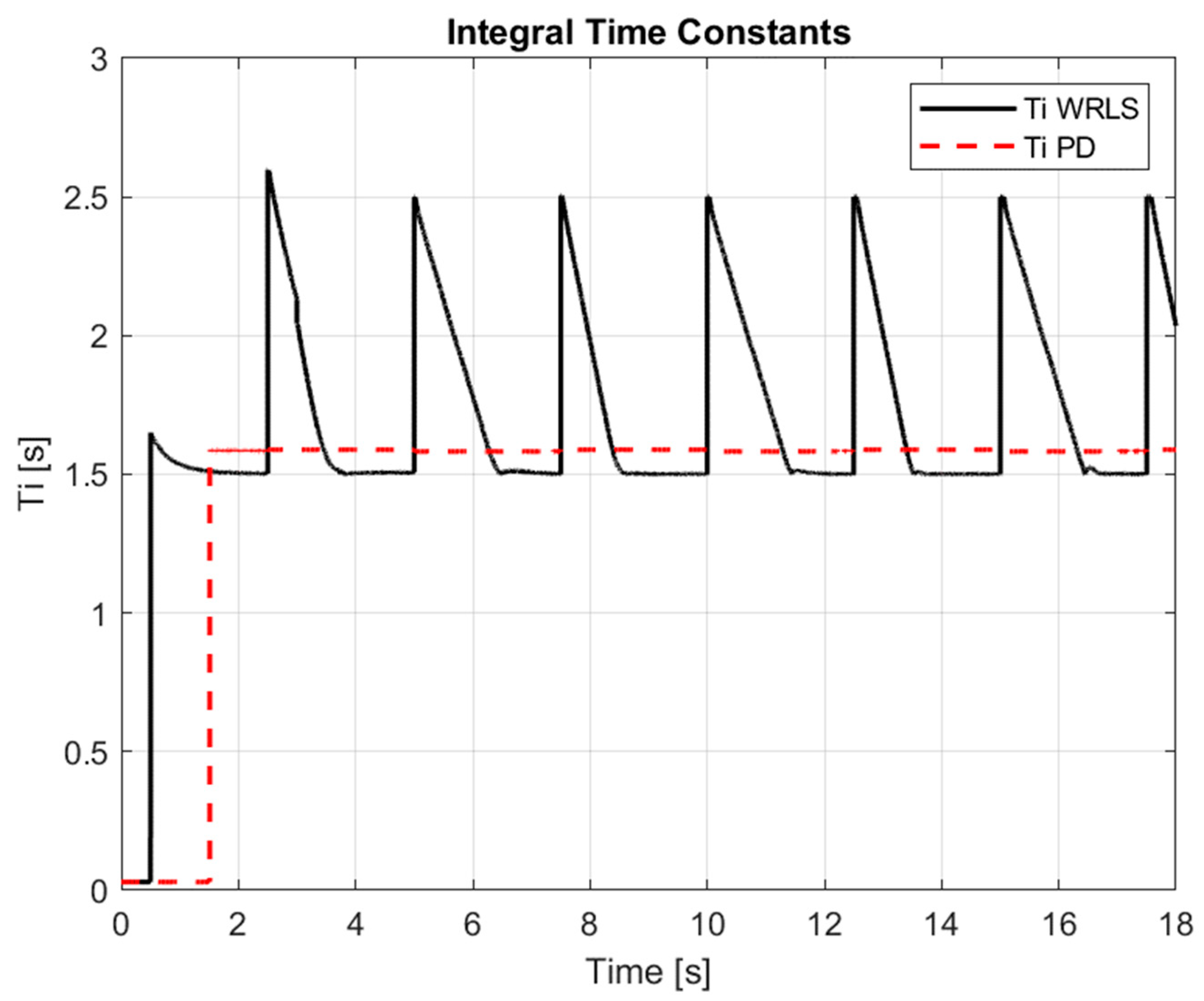
Figure 11.
Derivative time constants, .
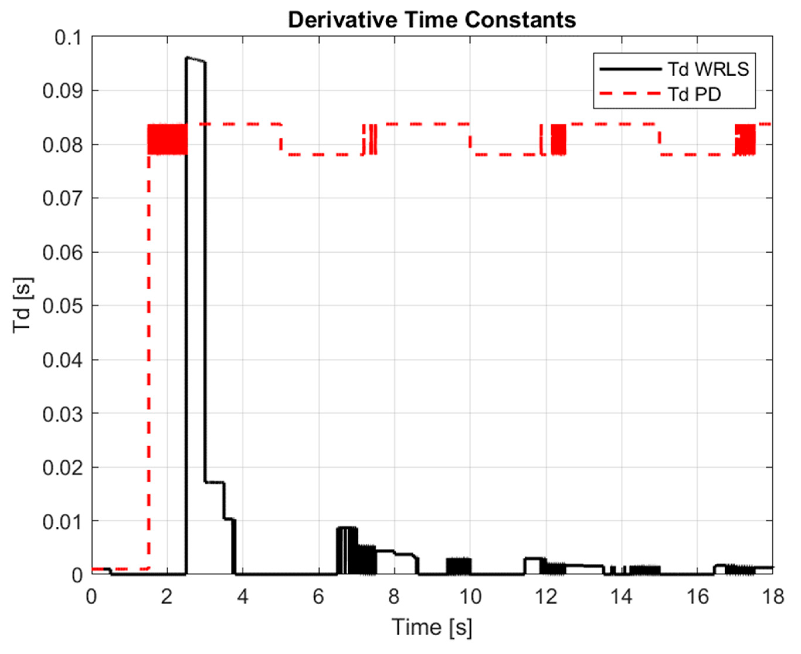
Figure 12.
Settling time, .
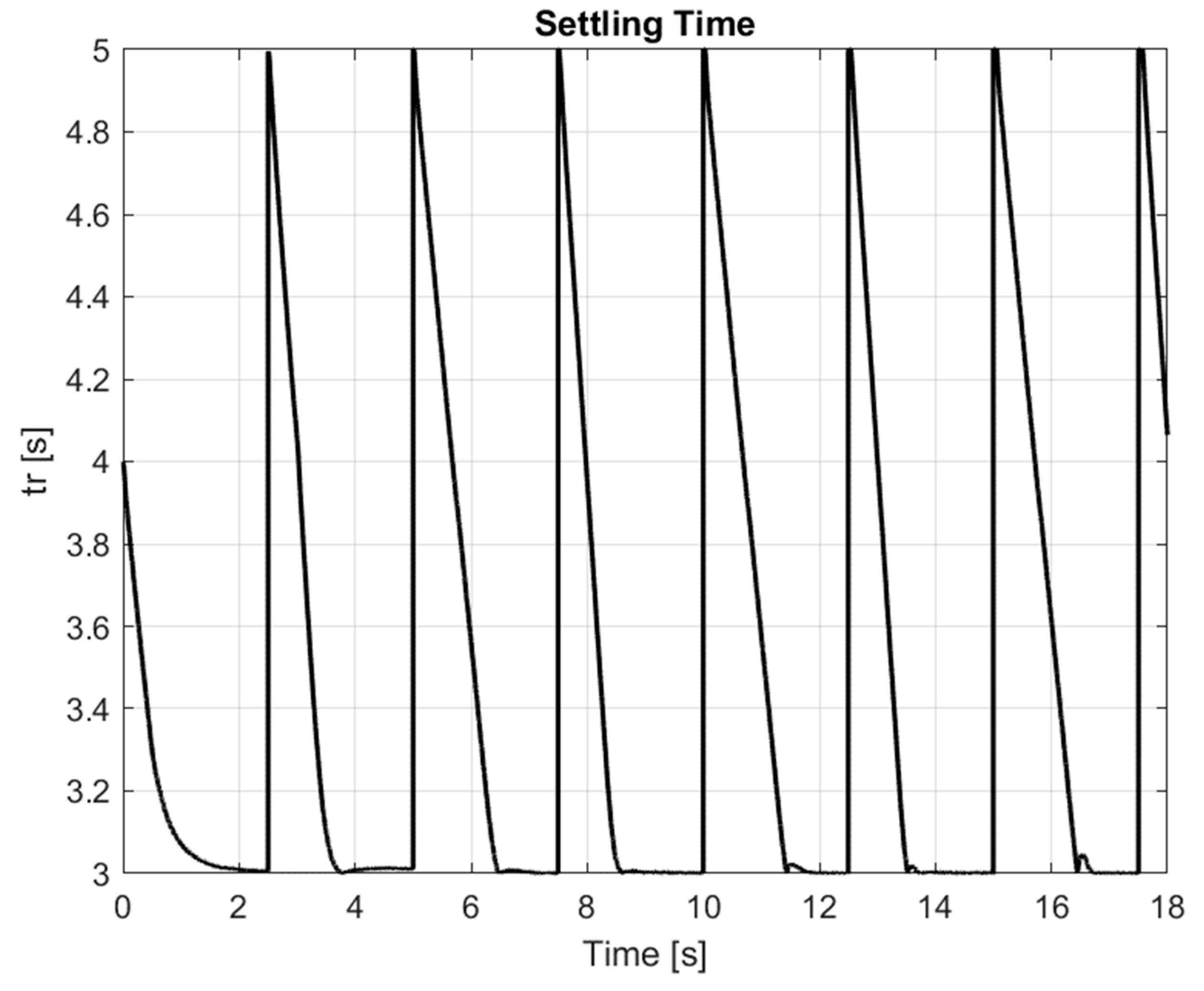
Figure 13.
Force, .
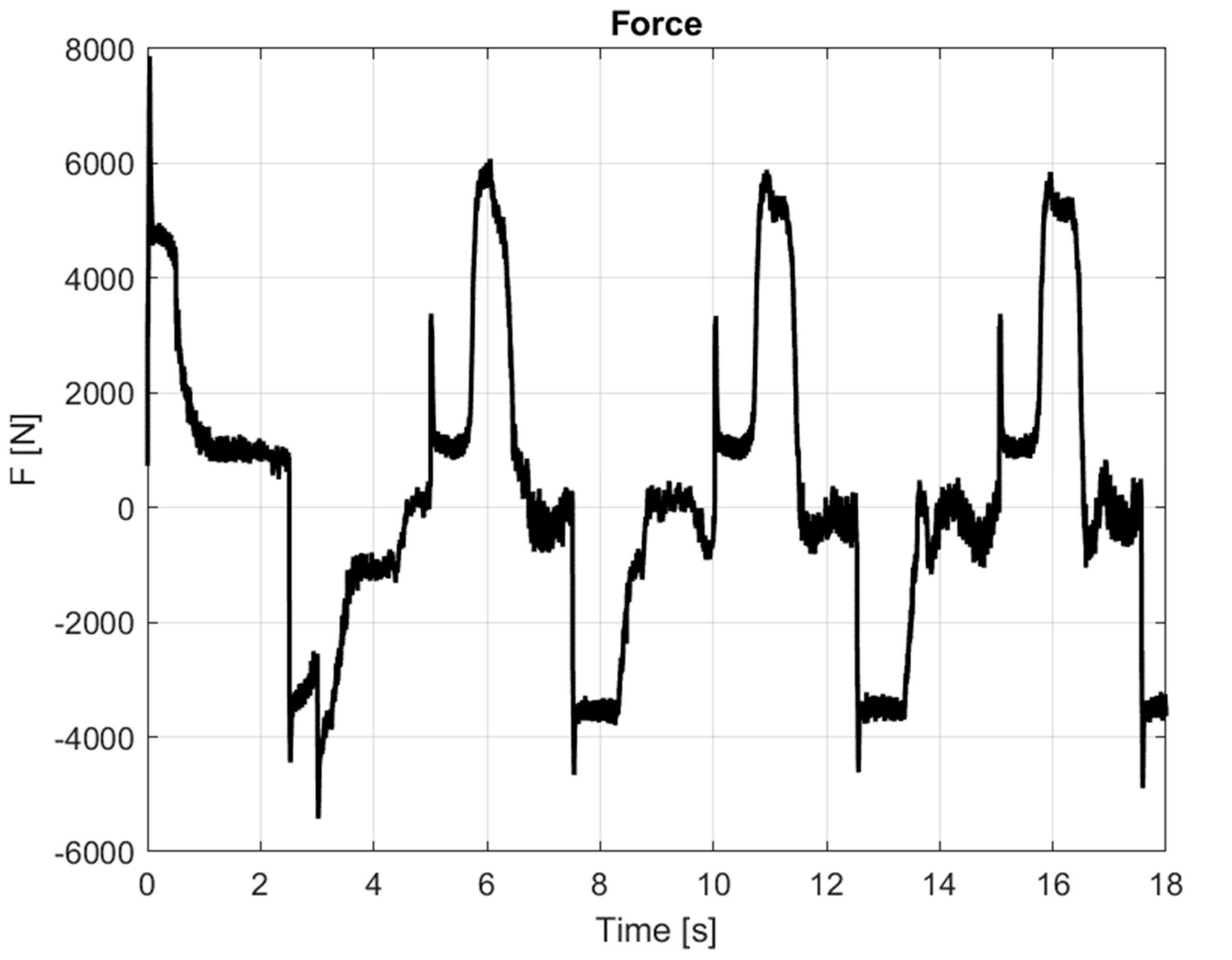
Table 1.
Comparison table of adaptive control methods.
| Method | Computational complexity | Stability | Performance in changing conditions | Ability to handle nonlinearity | Adaptation speed |
| MRAC | Medium | High | High for linear systems | Low | Medium |
| SMC | High | High | Excellent in disturbance conditions | Very good | Low |
| Fuzzy Control | Medium | Medium | Good in uncertain conditions | Medium | Medium |
| WRLS | Low-Medium | High | Very good in changing conditions | Medium | Very high |
| MPC | Very high | High | Excellent with an accurate model | High (if nonlinear MPC is used) | Medium |
Table 2.
Control results.
| Controller | [s] | Model | MAE [m] | Tracking error improvement[%] |
| PID | on-line | on-line | 0.0239288 | 18.8 |
| on-line | off-line | 0.0271719 | 7.8 | |
| 3 | off-line | 0.0294802 | 0.0 | |
| 3 | on-line | 0.0224433 | 23.8 | |
| PD | on-line | on-line | 0.0221932 | 24.4 |
| on-line | off-line | 0.0270030 | 8.0 | |
| 3 | off-line | 0.0293603 | 0.0 | |
| 3 | on-line | 0.0255266 | 13.0 | |
| P | on-line | on-line | 0.0238280 | 19.0 |
| on-line | off-line | 0.0269969 | 8.3 | |
| 3 | off-line | 0.0294408 | 0.0 | |
| 3 | on-line | 0.0223862 | 23.9 |
Table 3.
Table of control system performance metrics.
| Controller | [s] | Model | Overshoot [%] | Response time 95% [s] | Improvement in response time[%] |
| PID | on-line | on-line | 0.93 | 1.29 | 17.31 |
| on-line | off-line | -1.70 | 1.53 | 1.92 | |
| 3 | off-line | -1.91 | 1.56 | 0.00 | |
| 3 | on-line | 0.83 | 1.30 | 16.67 | |
| PD | on-line | on-line | 0.58 | 1.31 | 18.13 |
| on-line | off-line | -2.07 | 1.54 | 3.75 | |
| 3 | off-line | -2.39 | 1.60 | 0.00 | |
| 3 | on-line | 0.48 | 1.32 | 17.50 | |
| P | on-line | on-line | 0.71 | 1.30 | 15.03 |
| on-line | off-line | -1.39 | 1.49 | 2.61 | |
| 3 | off-line | -1.56 | 1.53 | 0.00 | |
| 3 | on-line | 0.53 | 1.32 | 13.73 |
Table 4.
Analysis of the statistical significance of control results.
| Controller | [s] | Model | ΔMAE [m] | p | 95% CI |
| PID | on-line | on-line | 0.00555 | 0.000000113 | [0.00482, 0.00628] |
| on-line | off-line | 0.00231 | 0.000083929 | [0.00158, 0.00304] | |
| 3 | on-line | 0.00704 | 0.000000018 | [0.00631, 0.00777] | |
| PD | on-line | on-line | 0.00717 | 0.000000015 | [0.00644, 0.00790] |
| on-line | off-line | 0.00236 | 0.000072339 | [0.00163, 0.00309] | |
| 3 | on-line | 0.00383 | 0.000001983 | [0.00310, 0.00456] | |
| P | on-line | on-line | 0.00561 | 0.000000104 | [0.00488, 0.00634] |
| on-line | off-line | 0.00244 | 0.000055952 | [0.00171, 0.00317] | |
| 3 | on-line | 0.00705 | 0.000000017 | [0.00633, 0.00778] |
Table 5.
Control results (N = 500).
| Controller | MAE [m] | |
| PD | 0.86 | 0.022864 |
| 0.88 | 0.022209 | |
| 0.89 | 0.022193 | |
| 0.90 | 0.022643 | |
| 0.91 | 0.022661 | |
| 0.95 | 0.022718 | |
| 0.97 | 0.022747 | |
| 0.99 | 0.022897 |
Table 6.
Control results (λ = 0.89).
| Controller | MAE [m] | |
| PD | 400 | 0.022261 |
| 500 | 0.021993 | |
| 600 | 0.022292 | |
| 700 | 0.022289 |
Table 7.
Statistical analysis of parameter estimation for different lambda values.
| Mean | CI | Mean | CI | Mean | CI | Mean | CI | |
| 0.86 | 0.024175 | 0.00037275 | 0.0024958 | 0.00021615 | 0.024314 | 0.00044089 | 0.016295 | 0.00048755 |
| 0.89 | 0.025087 | 0.00037400 | 0.0024956 | 0.00021615 | 0.024851 | 0.00043781 | 0.018499 | 0.00047666 |
| 0.90 | 0.024847 | 0.00036901 | 0.0024957 | 0.00021615 | 0.024600 | 0.00043925 | 0.015224 | 0.00049345 |
| 0.91 | 0.025134 | 0.00036966 | 0.0024955 | 0.00021615 | 0.024603 | 0.00043923 | 0.015287 | 0.00049309 |
| 0.95 | 0.026211 | 0.00036135 | 0.0024954 | 0.00021615 | 0.024832 | 0.00043792 | 0.015403 | 0.00049242 |
| 0.97 | 0.027001 | 0.00035555 | 0.0024954 | 0.00021615 | 0.024986 | 0.00043702 | 0.015614 | 0.00049121 |
| 0.99 | 0.027891 | 0.00034587 | 0.0024953 | 0.00021615 | 0.025176 | 0.00043593 | 0.016767 | 0.00048474 |
| σ | 0.001321 | 0.0000001 | 0.000284 | 0.001180 |
Disclaimer/Publisher’s Note: The statements, opinions and data contained in all publications are solely those of the individual author(s) and contributor(s) and not of MDPI and/or the editor(s). MDPI and/or the editor(s) disclaim responsibility for any injury to people or property resulting from any ideas, methods, instructions or products referred to in the content. |
© 2025 by the authors. Licensee MDPI, Basel, Switzerland. This article is an open access article distributed under the terms and conditions of the Creative Commons Attribution (CC BY) license (http://creativecommons.org/licenses/by/4.0/).
Copyright: This open access article is published under a Creative Commons CC BY 4.0 license, which permit the free download, distribution, and reuse, provided that the author and preprint are cited in any reuse.


