
Submitted:
06 May 2025
Posted:
06 May 2025
You are already at the latest version
Abstract
Aiming at the problems of excessive dependence on manual operations, unquantifiable parameters, low hoisting efficiency, and low level of automation and informatization in the lifting process of spacecraft, a novel cable-driven parallel automatic leveling robot with a two-stage adjustment function is proposed. It contains a cable-driven parallel mecha-nism and a counterweight compensation mechanism and has the advantages of high load-bearing capacity and better posture adjustment. Its kinematics and leveling perfor-mance are studied systematically. First, a geometric model of the robot is established, and the inverse position is derived. Second, the system's eccentric coordinates are solved based on the inclination angles of the moving platform. A theoretical model of the cable adjust-ment length is established according to the eccentric coordinates, and the cable adjust-ment scheme is analyzed and optimized. Third, according to the optimal cable adjust-ment scheme, the relationship between the inclination angles and the counterweight's adjustment displacement is established to better improve the leveling accuracy based on the force and torque balance principle. Finally, the kinematics and leveling performance are verified through MATLAB numerical calculations, ADAMS simulation and experi-mental study, proving that the robot could realize the hoisting and leveling task.
Keywords:
Cable-Driven Parallel Robot
; Counterweight Compensation Mechanism
; Kinematic Analysis
; Leveling Performance
1. Introduction
Hoisting equipment, especially the hoisting tools used for expensive or high-precision objects (such as satellites, aircraft, etc.), are indispensable auxiliary equipment in aerospace, weapons equipment, port transportation, and so on. They play an important role in leveling or adjusting posture during the hoisting process. Such objects generally have characteristics such as large structural weight, high requirements for smooth hoisting, an uncertain center of gravity, and high precision requirements for posture adjustment. At present, the hoisting equipment used in spacecraft generally has some problems, such as difficulty balancing operational performance and efficiency, over-reliance on manual experience, and a low degree of information and intelligence. [1]
In order to solve the above problems, it is necessary to research hoisting equipment that can achieve automatic adjustment. Currently, the equipment used for hoisting large objects is generally multiple mobile cranes, adopting a multi-point suspension mode, and adjusting the posture depending on the movement of the crane. For example, Zi Bin et al. [2] proposed a cable-driven parallel robot coordinated by four mobile cranes to solve complex tasks that a single crane is difficult to complete. The four-point collaborative leveling method is adopted for automatic leveling control for the CPRMCs platform with a PID controller. For conditions requiring single-point suspension, such as the indoor transfer or assembly of spacecraft, there are relatively few devices capable of automatic posture adjustment. According to the different leveling principles, automatic leveling robotic hoisting devices can be designed in various forms, such as main hoisting point mobile type [3], rope direct connection type [4,5], and counterweight compensation type [6,7]. The main hoisting point mobile type hoisting device achieves rapid adjustment of eccentricity through the movement of the main hoisting point, which can be realized using a two-dimensional sliding table structure [8] or a cable-driven parallel mechanism [9,10,11]. For instance, Tang et al. [3] developed an automatic leveling hoisting device that uses a two-dimensional sliding table to achieve the movement of the main hoisting point. An XY workbench is installed to adjust the hoisting point of the spreader, and an inclination sensor is used to measure the size and direction of the spreader’s inclination accurately. Although the measurement of the angle and the adjustment distance have been realized automatically, operations such as controlling the overhead crane and holding the spacecraft tightly still need to rely on manual labor. The operation process is complicated, requires high technical skills from the operators, and cannot achieve dynamic continuous adjustment.
Italian scholar Carlo Ferraresi et al. [12] designed a 9-rope 6-DOF cable-driven parallel mechanism, which can achieve 6-DOF posture adjustment of the motion platform. The spreader structure of the main hoisting point mobile type has the characteristics of a large adjustment range and quick posture adjustment. However, the movement of the main hoisting point requires the overhead crane to follow, which will bring a larger swing to the system and increase the operation difficulty. Rope direct connection type spreaders have the characteristic that the suspended object is directly connected with the adjusting ropes [13]. For example, the feed flexible cable support system of a 500-meter aperture spherical radio telescope (FAST) realizes the adjustments of position and posture of the end platform through a six-cable-driven parallel mechanism [14]. The RoboCrane, which is applied to the hoisting work of large component assembly, adjusts the posture of the suspended movable platform through six paired connected ropes [15]. This type of spreader has the characteristics of relatively simple structures, large load-bearing capacity, and high degrees of freedom, flexibility, and adaptability. which is suitable for applications requiring rapid response and extensive motion range. However, when lifting heavy loads, larger adjustment forces are needed, and the elasticity and swinging of the ropes may result in unstable lifting operations, so additional control and adjustments are required [16]. A counterweight-based spreader achieves posture adjustment through the movement of counterweights. For example, Zhang et al. [17] proposed a 3D crane leveling mechanism based on weight compensation technology, which is composed of a crane, ropes, a leveling box, and four ropes of the same length. The leveling box is divided into three parts, with all sensors, motors, and microcomputers installed in the middle control part and two compensation weights, along with two beams installed in the upper and lower execution parts, respectively. The adjustment of this type of spreader is safe and stable. However, with the increase in the weight of the suspended object, the compensation weight will significantly increase so that the self-weight and dimensions of the spreader will increase.
Therefore, for the designer, it is essential to consider the advantages and disadvantages comprehensively in practical applications and carry out reasonable design and selection. Aiming at the hoisting requirement of spacecraft with unknown center of mass, a rigid-flexible coupling cable-driven parallel robot spreader with a two-stage adjustment function combining the movement of the main hoisting point and counterweight is proposed in this paper. Its two-stage adjustment realizes through the cable-driven parallel mechanism and counterweight compensation mechanism. It has the characteristics of strong load-bearing capacity, large workspace, easy reconfiguration, and flexible scale. The length of cables or the displacement of counterweights can be adjusted automatically based on the inclination angles, and the desired posture requirements can be achieved. This design can solve the problem of insufficient automatic leveling ability of the existing automatic leveling robot.
Kinematic analysis of a mechanism is the premise of determining its workspace, studying its posture and pose, analyzing its motion performance, and optimizing its design and control. The kinematic and dynamic analysis of cable-driven parallel robots is always a hot and challenging problem in mechanism research. The principle of virtual work, based on the principles of work and energy conservation, provides an accurate relationship between posture and joint angles [18,19]. Wang et al. [20] proposed a cable-driven parallel mechanism with four sets of pulleys directly connected to the moving platform. The mapping matrix from the moving platform posture to cable lengths was derived by analyzing a single set of pulleys. Additionally, the velocity and acceleration formulas of the mechanism were solved according to the principle of virtual work. John et al. [21] proposed a spatial cable-driven two-degree-of-freedom joint with variable stiffness capability, and based on the screw theory, thoroughly analyzed the joint mobility and workspace. Palpacelli [22] enhanced the force controllability and static performance of industrial robots by introducing actuation redundancy to establish kinematic and static models. Jia et al. [23] presented a method for solving the coupled cable-driven serial-parallel robotic arm using iterative Jacobian pseudoinverse computation. Li [24] established the kinematic model and trajectory error of the end effector for parallel cable-driven robots using the closed vector method and the theory of differential kinematics. Chesser et al. [25] utilized a cable-driven parallel robot for concrete additive manufacturing, establishing a kinematic model via the vector closure method, ultimately obtaining the reachable workspace of the end-effector. Through the analysis of the above methods, it can be observed that the closed vector method has the advantages of simplicity and convenience when analyzing the kinematics of cable-driven parallel mechanisms. In this paper, the kinematic model of the mechanism is established based on the closed vector method, and the positional solution is obtained. Then, an innovative approach is introduced to solve the adjustment amounts through torque balance equations. The required adjustment amounts when the mechanism reaches the given positions are derived from the difference in the positions of the counterweights between the current position and the critical equilibrium states according to the balance assumption and steady-state approximation methods. The algorithm iterates according to the current inclination angles of the platform to eliminate the inevitable errors caused by flexible cables until the platform meets the predefined evaluation criteria.
The remaining sections of the article are outlined as follows: The second section mainly introduces the kinematic model of the mechanism. Firstly, the three-dimensional model and structural schematic of the cable-driven parallel automatic leveling robot are given, and the favorable position solution of the mechanism is derived using the closed vector method. Then, to ensure adjustment precision, an optimized adjustment scheme with the preferred selection of cables is proposed to ensure the stability of the spacecraft hoisting process. Finally, the adjustment amounts of the counterweights are solved based on force and torque balance equations, and the two-stage high-precision mechanism adjustment is completed. In the third section, MATLAB numerical calculation and ADAMS simulation are carried out on the automatic leveling robot model. In the fourth section, the experimental prototype has been built and experimental study has been carried out. The results validate the correctness of the leveling algorithm and the theoretical models.
2. Kinematic Modeling of Cable-Driven Parallel Automatic Leveling Robot
2.1. Structural Characteristics of Cable-Driven Parallel Automatic Leveling Robot
The three-dimensional model of the newly designed cable-driven parallel automatic leveling robot is illustrated in Figure 1. (a) depicts the overall three-dimensional structure of the robot, while (b) provides a detailed magnification of a single drive branch. The robot consists of a two-stage adjustment system, including the first-stage initial adjustment module with a cable-driven parallel mechanism and the second-stage accurate adjustment module with a counterweight compensation mechanism. It can achieve three degrees of freedom adjustments in pitch, yaw, and vertical displacement. Each of the three inclined tension cables has one end connected to the connection point of the screw-nut mechanism through a fixed pulley on the cable-driven platform, and the other end is connected to the main hoisting point. Each branch is driven by a servo motor to achieve changes in the cable length through the motion of the screw-nut mechanism. The counterweights are arranged in a cross-shaped pattern on the counterweight platform, with each direction being driven by a servo motor to propel two counterweights along guide rails bidirectionally. The four vertical suspension cables are connected with one end to the counterweight platform and the other end to the suspended object. The robot mechanism employs a modular design approach, which is easy to install, flexible to disassemble, and convenient to debug. An inclination sensor is positioned on the cable-driven platform to measure the inclination angles of the moving platform. Tension sensors are installed at the connections between the four vertical suspension cables and the moving platform to measure the tension of these cables in real time. The system can continuously monitor the inclination of the suspended object and make adjustment strategies according to the information of the inclination sensor and tension sensors.
During the first-stage initial adjustment process of the robot, the main hoisting point is moved by changing the cable length of the cable-driven parallel mechanism, and the projection position of the main hoisting point is adjusted to the eccentric position based on the inclination angles of the moving platform, so as to realize the levelness adjustment of the suspended object. Due to the need for the crane to follow the movement of the main hoisting point and considering the precision affected by crane operation accuracy, a second-stage accurate adjustment module with four counterweights is designed to further enhance the leveling precision of the mechanism. When the system detects that the platform inclination angles are less than the set threshold, the adjustment of the cable-driven parallel mechanism is halted, and the counterweights are driven to carry out the second-stage accurate adjustment until the specified evaluation criteria are met.
Figure 2 illustrates the structural configuration and force diagrams of the cable-driven automatic leveling robot. (a) represents the overall system structure and a simplified force diagram, (b) provides a schematic diagram of the counterweight structure, and (c) illustrates the pulley structure. The moving platform contains cable-driven platform m1 with center point o, and the counterweight platform m2 with center point o2. The centers of the pulleys connected to the three cable-driven branches are denoted as Bi(i=1,2,3), forming a symmetrical distribution along a circular path. The distance from point Bi to o is represented as R. A coordinate system {B}: o-xByBzB is attached on o with yB points to B1, xB vertical yB extends horizontally to the right, and zB is determined according to the right-hand screw rule. The coordinate system attached to the main hoisting point O is denoted as {A}: O-xAyAzA. Initially, {A} shares the same axis directions with {B}. The inclination angles of the moving platform are denoted as α for rotation around the X-axis and β for rotation around the Y-axis. The center points of each counterweight are denoted as Pi(i=1,2,3,4). The center point of the four counterweights' center plane is denoted as o1. The distances from Pi to o1 are represented as lpi (i=1,2,3,4). Initially, the distances from P1 and P3 to o1 are both lpx0, while the distances from P2 and P4 to o1 are both lpy0, and the height from o1 to o is hP. The height from the center point o2 to o is hc. A coordinate system attached to o2 is denoted as {D}: o2-xDyDzD. In this coordinate system, xD points to P3, yD points to P4, and zD is determined according to the right-hand screw rule. {D} and {B} coordinate axes are always in the same direction. The connection points of the vertical suspension cables to the counterweight platform are denoted as Di (i=1,2,3,4). The distance from Di to o2 is Rd, and these points are symmetrically distributed along a circular path. The distance from O to Bi is Li (i=1,2,3). The points where the cables intersect with the pulley are labeled as Ki (i=1,2,3). The distance from O to Ki is LKiO(i=1,2,3). The distance between o and O is LoO. The radius of the pulley is Rp. The acute angle between the line BiKi and the line Bio is θi (i=1,2,3).
2.2. Leveling Kinematics Analysis of Cable-Driven Parallel Mechanism
According to the adjustment principles of the designed mechanism, adjusting the length of cables can realize an initial adjustment in the horizontal orientation of the suspended load. The inverse kinematics of the cable-driven parallel mechanism is described as follows: given the position of the moving platform m1 in coordinate system {A} as o (Xo, Yo, Zo) and the orientation (α, β, γ), the task is to solve the lengths Li. {B} rotates α around X-axis and β around Y-axis with respect to {A}. Utilizing ZYX Euler angles, the rotational transformation matrix between the two coordinate systems is expressed as:
Coordinates of Bi, Di, o1 and o2 are represented in {B} and {A}, respectively, as follows:
In the equation, o represents the coordinates of o in {A}.
Based on the geometric relationships in Figure 2(c), the angles θi(i=1,2,3) at the pulley locations, distance LoO between o and O can be solved as:
Coordinates of Ki, position vectors LBiKi, LKiO and unit direction vectors of cables δLKi (i=1,2,3) are derived as:
According to the closed vector method, the length vector of the cable Li (i=1,2,3) and its length Li can be solved as:
Assuming the projection coordinates of the main hoisting point O on the moving platform m1 is BA=[m n 0]T, and the position vector from O to the projection point A is BlOA=[0 0 h]T, then, the position vector BlABi (i=1,2,3) from Bi to A can be expressed as follows:
According to the vector closed-loop relationship of the vertical line from O to the moving platform m1, the line connecting point A with Bi, and the cable length. The expression of the cable length in {B} BLi (i=1,2,3) is:
Hence, the lengths of the cables in different positional states can be solved based on relevant structural parameters and system state parameters.
To carry out the leveling operation, the cable adjustments amount can be solved based on the cable lengths before and after movement. The approach is to calculate the eccentric position PC based on the platform inclination angle, and determine the movement of the main hoisting point according to PC to calculate the new cable lengths, and then the cable adjustment amount can be derived based on the difference of cable lengths in the two cases.
When the cable lengths are known, the eccentric coordinates (m, n), the vertical height h and the coordinates of the eccentric position PC in {B} denoted as BPC can be solved as:
When adjust the eccentric position coordinates to the target, the projection point of the main hoisting point coincides with the eccentric position. At this point, the new adjusted cable lengths, denoted as BLiN (i=1,2,3), can be solved using the Formula (7):
Here, BlPBi and BlO´P represent the position vectors from PC to Bi, and from the main hoisting point to the projected point after moving to the target position in {B}, respectively. ∆h is the change in the height of the main hoisting point.
From this, the cable adjustment amount ∆Li (i=1,2,3) is derived as:
The variation in cable lengths leading to changes in the height of the main hoisting point, in order to ensure solution determinacy and guarantee adjustment precision, the adjustment process limits the changes to at most two cables each time. Therefore, optimization selection of the adjustment scheme is required. To ensure safety and minimize horizontal forces on the suspended load during the adjustment process, the cables far from the eccentric position will be adjusted preferentially. This will ensure the cables only extend without retract. Based on this, the optimal cable adjustment scheme is illustrated in Figure 3.
2.3. Leveling Kinematic Analysis of Counterweight Compensation Mechanism
To ensure the precision and stability of the adjustment process, a counterweight compensation mechanism is employed for accurate adjustment in small inclination angles. The current positions of the counterweights are solved based on the current inclination angles. The theoretical positions of the counterweights are calculated when the system adjusts the inclination angles to zero. The differences in counterweight positions between these two cases are the required adjustment distances.
(1) Current Positions Calculation of the Counterweights
The positions of the four counterweights are represented as:
In Equation (11), lpi(i=1,2,3,4) is the distance from the counterweight Pi to o1, and the following relationship holds:
Where lpis represents the current positions, ∆lpx and ∆lpy denote the changes in the counterweight's current positions compared to the initial positions. The coordinates of the counterweight positions in {A} are expressed as:
There exists the following force and torque equilibrium equations in this robot system:
Here, The above equations represent the corresponding relationship between the tension in inclined cables and the positions of counterweights. Additionally, considering the elasticity of cables, the following deformation coordination equations are derived:
In Equation (15), δL1, δL2, and δL3 represent the deformation of each inclined cable, and Fi represents the magnitude of the tension. Their expressions are: δLi=FiLi/(EA1), , where E is the elastic modulus of the cable, and A1 is the cross-sectional area of the cable.
Considering the moment equilibrium about the vertical line passing through O, we can derive:
By simultaneously solving Equations (13) to (16), the tension forces in the cables and the displacement of the counterweights can be derived.
(2) Theoretical Positions Calculation of Counterweights After Leveling
After leveling, assuming the tension in the vertical suspension cables is still FDi, the theoretical positions of the counterweights when the system is horizontal are solved as:
Where lpil represents the distance from the center point to the theoretical positions of the counterweights after leveling, and ∆lpx1, ∆lpy1 represents the changes in the theoretical positions of the counterweights after leveling compared to the initial positions.
At the horizontal position, where both α and β are zero, the tension in the cables and the positions of the counterweights can be solved by Equation (13)-(16).
(3) Solve of Counterweight Displacements
The purpose of moving counterweight is to achieve two-stage high-precision leveling. Ideally, the inclination angles of the moving platform are double 0°, and the counterweight positions are solved based on the torque balance condition. The solution processes are as follows:
1) Solve the current positions of the counterweights lpis, that is, the change amounts ∆lpx and ∆lpy are obtained;
2) Set the angular values α and β of the X and Y-axes to 0°, that is the angles when the robot system achieves the ideal leveling state;
3) Solve for the tension force Fi of the inclined cables and the unit vector δLKi of the cable based on mechanical analysis of the automatic leveling robot system;
4) According to the process of solving the current positions of the counterweights, the theoretical positions of the counterweights after leveling are solved. The distance from each counterweight position to the center o1 is lpil. The solution expression is shown in Equation (17), and ∆lpx1, ∆lpy1 represent the changes in the counterweight positions when it moves to the ideal balance state.
5) Adjust the counterweights by moving them based on the difference between the two changes;
6) Measure the X and Y-axis angles α and β again. If the specified angle threshold is not reached, record the current positions of the counterweights and proceed with steps (1)-(6) iteratively until the desired angles are met.
3. Simulation Analysis of Cable-Driven Parallel Automatic Leveling Robot
To validate the effectiveness, feasibility, and correctness of the leveling algorithm, simulation analysis during the leveling process of the cable-driven parallel mechanism and counterweight compensation mechanism is conducted. For specific instances, MATLAB numerical calculations and ADAMS simulations are carried out. The structural parameters, mass parameters, and working loads applied on the four vertical suspension cables are shown in Table 1. The simulation model of the robot is established using ADAMS software, as shown in Figure 4(a). To simulate the posture after completely lifting the spacecraft, loads of magnitude FD1=FD4 =20KN and FD2=FD3=50KN are added to the end of the four vertical suspension cables. The loads are applied in the vertically downward direction. The two-stage adjustment conversion threshold is set to 1°. After applying external forces, the moving platform inclines with angles α=4.817° and β=4.819°, as shown in Fig 4(b). The position and posture of the platform and the lengths of the inclined cables are measured and substituted into equation (5) for calculation.
Based on the cable adjustment algorithm, the cable adjustment values are calculated in MATLAB, and the results are: ∆L1=191.38mm, ∆L2=143.86, and ∆L3=0mm. According to this, by controlling the motion of the robot using these adjustments to the cables, the position and posture of the platform after the first adjustment of the inclined cables are shown in Figure 4(c). The simulated measurement results are obtained in ADAMS by setting corresponding parameters for the simulation. The curves depicting the changes in inclination angles, cable lengths, and cable forces are shown in Figure 5. During the external force loading process, the variation of cable forces and the relative errors between analytical solutions and simulation solutions are shown in Figure 6(a),(b), respectively, with a maximum relative error of less than 0.87%. After the first adjustment of the cable-driven parallel mechanism, the calculated inclination angles of the moving platform become α=1.423° and β=1.339°, with a significant reduction. The platform posture is depicted in Figure 4(c).
At the end of one iteration of the cable adjustment, the system detects that the platform inclination has not reached the threshold of 1°, the rope adjustment algorithm continues work. The current posture information is recorded, and based on the iterative calculation of the cable adjustment algorithm, the adjustment amounts for the cables are solved to be ∆L1=62.122mm, ∆L2=47.135, ∆L3=0mm. The adjusted platform posture is shown in Figure 4(d). At this time, the inclination angles are α=0.658°, and β=0.032°, which are below the set threshold. The system will exit the cable control loop and begin the counterweight adjustment algorithm. Based on the current posture, the adjustment amounts for the counterweights are calculated as ∆lx=-25mm and ∆ly=512.7mm. The positions of the counterweights before and after adjustment are shown in Table 2. After the counterweight adjustment, the inclination angles are α=0.103°, β=0.022°, and the platform posture is shown in Figure 4(e). This satisfies the horizontal accuracy required for the spacecraft hoisting. The counterweight adjustment is completed, and the system exits the loop. The postures of the moving platform during the two-stage adjustment are shown in Table 3.
Based on the analyzed results, it is evident that the changes in cable lengths, platform angles, and cable forces during the adjustment process are in accordance with reality. The analytical values and simulated values of cable forces are in good agreement, and the curves are smooth. The maximum relative error is less than 0.87%. This proves the correctness of the theoretical model and computational results. Also, it proves the feasibility of the proposed two-stage adjustment method.
4. Simulation Analysis of Cable-Driven Parallel Automatic Leveling Robot
4.1. Initial Adjustment Experiment of Cable-Driven Parallel Mechanism
To further verify the practical application effect, the experimental prototype has been built. The prototype of initial adjustment cable-driven parallel mechanism is shown in Figure 7. Its moving platform is made of aluminum alloy. There are three linear modules driven by servo motors arranged at 120° on the moving platform and an inclination sensor arranged on the center. The posture of the suspended object is considered as the same with the moving platform, so the angles measured by the sensor represent the posture of the suspended object. Each steel cable can be driven by the corresponding module and the main lifting point can be changed by a winch. A PLC controller is used for the motion control. The module displacement is precisely measured by receiving A/B phase pulses from the feedback of the servo motor, so as to determine the cable length.
To verify the actual leveling performance of the designed robot, a dynamic hoisting and posture adjustment experiment has been conducted using a PID controller. During the experiment, set eccentricity randomly, then lift the device upward slowly. In this process, values of inclination sensor are read and recorded in real time and posture of moving platform is adjusted through the designed control system when the inclination angles exceed ±1°. The adjustment will be finished until the platform fully off the ground and the inclination angles remain within the target range.
Here, two sets of experiments are conducted shown as situations a and b.
Situation a. The eccentric position PC (x, y) satisfies: ,and.
The experimental model is shown in Figure 8(a),(b). In this situation, according to the adjustment algorithm, ΔL1 is set to 0, lengths of L2 and L3 should be adjusted. During the adjustment, the angle values of the inclination sensor before and after filtering are shown in Figure 9(a),(b), cable lengths are shown in Figure 9(c). After adjustment, values of inclination sensor are stable within ±1°, which is consistent with the reality.
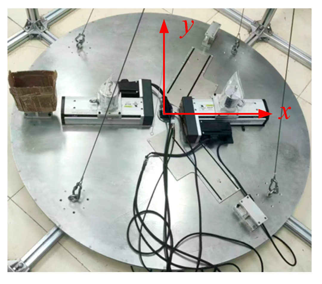
Situation b. The eccentric position PC (x, y) satisfies:, .
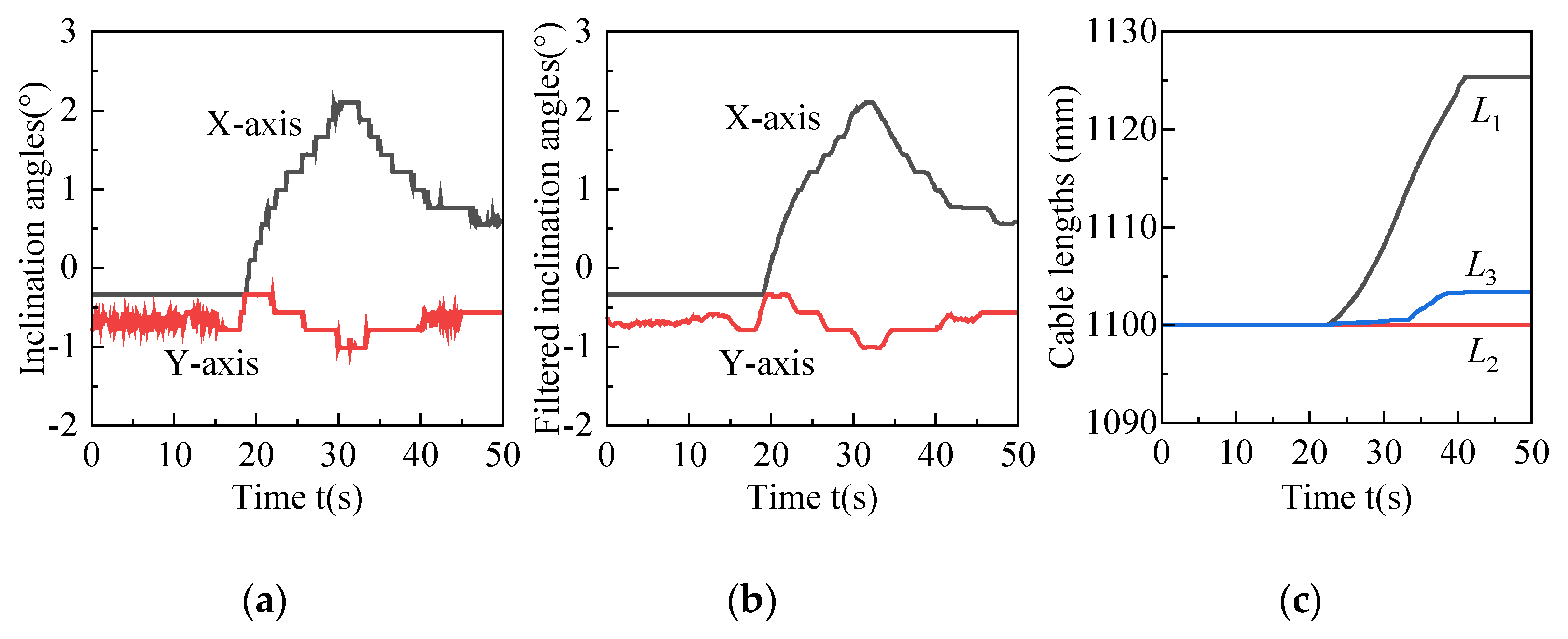
The experimental model is shown in Fig. 10(a) and 10(b). In this situation, ΔL2 is set to 0, lengths of L1 and L2 should be adjusted. During the adjustment, the angle values of the inclination sensor before and after filtering are shown in Fig. 11(a) and 11(b), cable lengths are shown in Fig. 11(c). After adjustment, values of inclination sensor are stable within ±1° too.
From the results we can know that: For situation a, the angles of X-axis changed from maximum -2.79° to the stable -0.56° and angles of Y-axis changed from maximum 1.44° to the stable -0.12°. During this process, the length of cable L1 remained constant, length of cable L2 increased from 1100 mm to 1152.11 mm, and length of cable L3 increased from 1100 mm to 1110.96 mm. For situation b, the angles of X-axis changed from maximum 2.10° to the stable -0.59° and angles of Y-axis changed from maximum -1.01° to the stable -0.56°. During this process, the length of cable L3 remained constant, the length of cable L1 increased from 1100 mm to 1125.38 mm, and the length of cable L2 increased from 1100 mm to 1103.37 mm. The experimental results are in accordance with the reality.
Figure 11.
Experimental result (a) The angle values of the inclination sensor before filtering; (b) The angle values of the inclination sensor after filtering; (c) Cable lengths.
Figure 11.
Experimental result (a) The angle values of the inclination sensor before filtering; (b) The angle values of the inclination sensor after filtering; (c) Cable lengths.
4.2. Accurate Adjustment Experiment of Counterweight Compensation Mechanism
To verify the actual leveling performance of counterweight compensation mechanism, this study further conducts dynamic adjustment experiments on the counterweight compensation prototype using a PID controller. The experiment prototype model is shown in Figure 16.
Figure 12.
Prototype model of the counterweight compensation mechanism.
Because of the symmetry and independence of X-axis and Y-axis in adjustment algorithm, there are only two linear modules arranged in X direction to save costs. Actually, it does can verify the feasibility. There are four fixed cable lengths connect the main hoisting point and moving platform. One counterweight with 2kg is arranged on each linear module. When the linear module moves, the counterweight moves with it. Based on the counterweight adjustment algorithm, a PLC program is written to control the movement of the linear modules. The adjustment is considered to be finished when inclination angles are stable within 0.11°. Initial position of each counterweight is 50mm away from the bottom of the corresponding module. Two modules move synchronously.
In order to better observe the leveling effect, the moving platform is lifted in a fully suspended status. Here, two sets of experiments are conducted with two different situations. One is an initial inclination angle of 0.55° in X direction. The other is an initial inclination angle of -0.34° in X direction. During the experiment, the angle values of the inclination sensor before and after filtering of the two situations are shown in Figure 13a,b and Figure 14a,b, respectively. The counterweight positions are shown in Figure 13c and Figure 14c.
In the first situation, inclination angles vary from 0.55° to 0.11°, counterweight position has changed from 50mm to 81.16mm. In the second situation, inclination angles vary from -0.34° to -0.11°, counterweight position has changed from 50mm to 34.89mm. Both positive and negative inclinations in X direction can realize the requirement adjustment. The threshold judgment prevents overshooting and oscillations. Although there exists noise and delay in the PLC signal acquisition, the angle values after moving average filtering can be used for smooth adjustment.
5. Conclusions
A new configuration of a cable-driven parallel automatic leveling robot was proposed, which can achieve 3-DOF adjustments in pitch, yaw, and vertical movement. This design meets the requirements for automatic leveling operations during the hoisting process of the spacecraft. Based on the closed vector method and the principle of force equilibrium, the kinematic models of the cable-driven parallel mechanism and counterweight compensation mechanism were established, and the corresponding relationships between the posture of the moving platform and the adjustments of cable lengths and counterweight movements were derived. Kinematic simulation analysis of the leveling process was conducted by using ADAMS software. The leveling performance further verified through experiments. The results showed that the proposed two-stage adjustment algorithms can achieve the desired leveling goals. The leveling accuracy is less than ±0.11° after adjustment, meeting the accuracy requirements. Results validate the correctness of the established theoretical model, and provides a theoretical basis and reference for the optimization design and precise control of the robot in the future.
Author Contributions
Zhuohong Dai and Ran Chen conceived and designed the study. Zhuohong Dai, Nan Liu and Tengfei Huang performed kinematic analysis. Tengfei Huang and Weikang Lv conducted reference review. Nan Liu, Xiangfu Meng and Tengfei Huang performed simulation analysis. Nan Liu and Xiangfu Meng performed experimental study. Zhuohong Dai, Nan Liu, Tengfei Huang and Weikang Lv wrote the article.
Funding
This work was supported by the Open Foundation of Tianjin Key Laboratory of Microgravity and Hypogravity Environment Simulation Technology (Grant No. WDZL-2021-04).
Data Availability Statement
The data presented in this study are available on request from the corresponding author. The data are not publicly available due to privacy.
Conflicts of Interest
The authors declare no conflicts of interest.
References
- Wang, P.; Zhang, X.; Xing, T.; Liu, C.; Zhang, S. Development and application of lifting and leveling system for space station. J. Phys. Conf. Ser. 2019, 1314, 012092. [Google Scholar]
- Zi, B.; Lin, J.; Qian, S. Localization, obstacle avoidance planning and control of a cooperative cable parallel robot for multiple mobile cranes. Robot. Comput. Integr. Manuf. 2015, 34, 105–123. [Google Scholar] [CrossRef]
- Tang, L.; Liu, Z.; Zou, L.; Zheng, P.; Liu, F. Simulation analysis of spacecraft automatic leveling and equalizing hoist device based on hanging point adjustment. IOP Conf. Ser. Mater. Sci. Eng. 2018, 392, 062042. [Google Scholar] [CrossRef]
- Khadem, M.; Inel, F.; Carbone, G.; Tich, A.S.T. A novel pyramidal cable-driven robot for exercising and rehabilitation of writing tasks. Robotica. 2023, 41, 3463–3484. [Google Scholar] [CrossRef]
- Cai, Q.; Chen, D.; Yang, N.; Li, W. A Novel Semi-Spar Floating Wind Turbine Platform Applied for Intermediate Water Depth. Sustainability 2024, 16, 1663. [Google Scholar] [CrossRef]
- Imanberdiyev, N.; Sood, S.; Kircali, D.; Kayacan, E. Design, development and experimental validation of a lightweight dual-arm aerial manipulator with a COG balancing mechanism. Mechatronics. 2022, 82, 102719. [Google Scholar] [CrossRef]
- Zhang, Y.; Guo, D.; Yang, Y. Design and Experimental Validation of a Micro-Newton Torsional Thrust Balance for Ionic Liquid Electrospray Thruster. Aerospace 2022, 9, 545. [Google Scholar] [CrossRef]
- Zivanovic, S.; Tabakovic, S.; Zeljkovic, M.; Dimic, Z. Modelling and analysis of machine tool with parallel–serial kinematics based on O-X glide mechanism. J. Braz. Soc. Mech. Sci. Eng. 2021, 43, 456. [Google Scholar] [CrossRef]
- Qian, S.; Zhao, Z.; Qian, P.; Wang, Z.; Zi, B. Research on workspace visual-based continuous switching sliding mode control for cable-driven parallel robots. Robotica. 2024, 42, 1–20. [Google Scholar] [CrossRef]
- Ghrairi, K.; Lamine, H.; Bennour, S.; Chaker, A. Camera-based control system of a planar cable-driven parallel robot intended for functional rehabilitation. Robotica. 2024, 1–20. [Google Scholar] [CrossRef]
- Wang, R.; Li, Y. Analysis and multi-objective optimal design of a planar differentially driven cable parallel robot. Robotica. 2021, 39, 1–17. [Google Scholar] [CrossRef]
- Ferraresi, C.; De Benedictis, C.; Pescarmona, F. Development of a haptic device with wire-driven parallel structure. Int. J. Automot. Technol. 2017, 11, 385–395. [Google Scholar] [CrossRef]
- Rasheed, T.; Long, P.; Caro, S. Wrench-feasible workspace of mobile cable-driven parallel robots. AMSE J. Mech. Robot. 2020, 12, 031009. [Google Scholar] [CrossRef]
- Tang, X.; Yao, R. Dimensional design on the six-cable driven parallel manipulator of FAST. AMSE J. Mech. Des. 2011, 133, 111012. [Google Scholar] [CrossRef]
- Lytle, A.M.; Saidi, K.S.; Bostelman, R.V.; Stone, W.C.; Scott, N.A. Adapting a teleoperated device for autonomous control using three-dimensional positioning sensors: Experiences with the NIST RoboCrane. Autom. Constr. 2004, 13, 101–118. [Google Scholar] [CrossRef]
- Cao, X.; Meng, C.; Zhou, Y.; Zhu, M. An improved negative zero vibration anti-swing control strategy for grab ship unloader based on elastic wire rope model. Mech. Ind. 2021, 22, 45. [Google Scholar] [CrossRef]
- Zhang, X.; Yi, J.; Zhao, D.; Yang, G. Modelling and control of a self-leveling crane. ICMA 2007, Harbin, China, Aug 5–8 2007, 2922–2927.
- Zhang, X.; Wang, H.; Rong, J.; Niu, J.; Tian, J.; Li, S. Dynamic modeling of a class of parallel-serial mechanisms by the principle of virtual work. Meccanica. 2023, 58, 303–316. [Google Scholar] [CrossRef]
- Chen, M.; Zhang, Q.; Ge, Y.; Qin, X.; Sun, Y. Dynamic analysis of an over-constrained parallel mechanism with the principle of virtual work. Math. Comput. Model. Dyn. Syst. 2021, 27, 347–372. [Google Scholar] [CrossRef]
- Wang, H.; Kinugawa, J.; Kosuge, K. Exact kinematic modeling and identification of reconfigurable cable-driven robots with dual-pulley cable guiding mechanisms. IEEE/ASME Trans. Mechatron. 2019, 24, 774–784. [Google Scholar] [CrossRef]
- John, I.; Mohan, S.; Wenger, P. Kinetostatic analysis of a spatial cable-actuated variable stiffness joint. ASME J. Mech. Robot. 2024, 16, 091003. [Google Scholar] [CrossRef]
- Palpacelli, M. Static performance improvement of an industrial robot by means of a cable-driven redundantly actuated system. Robot. Comput. Integr. Manuf. 2016, 38, 1–8. [Google Scholar] [CrossRef]
- Jia, L.; Zhang, L.; Mu, Z.; Gao, M.; Zhang, N.; Song, R. A kinematic-decouple model for cable-driven manipulators with series-parallel coupling relationship. Mech. Solids. 2023, 58, 912–921. [Google Scholar] [CrossRef]
- Li, Y.; Xue, Y.; Yang, F.; Cai, H.; Li, C. Comprehensive compensation method for motion trajectory error of end-effector of cable-driven parallel mechanism. Machines. 2023, 11, 520. [Google Scholar] [CrossRef]
- Chesser, P.C.; Wang, P.L.; Vaughan, J.E.; Lind, R.F.; Post, B.K. Kinematics of a cable-driven robotic platform for large-scale additive manufacturing. AMSE J. Mech. Robot. 2022, 14, 021010. [Google Scholar] [CrossRef]
Figure 1.
Two-stage adjustment automatic leveling robot. (a) 3D model of the mechanism; (b) Drive branch of the cable.
Figure 1.
Two-stage adjustment automatic leveling robot. (a) 3D model of the mechanism; (b) Drive branch of the cable.
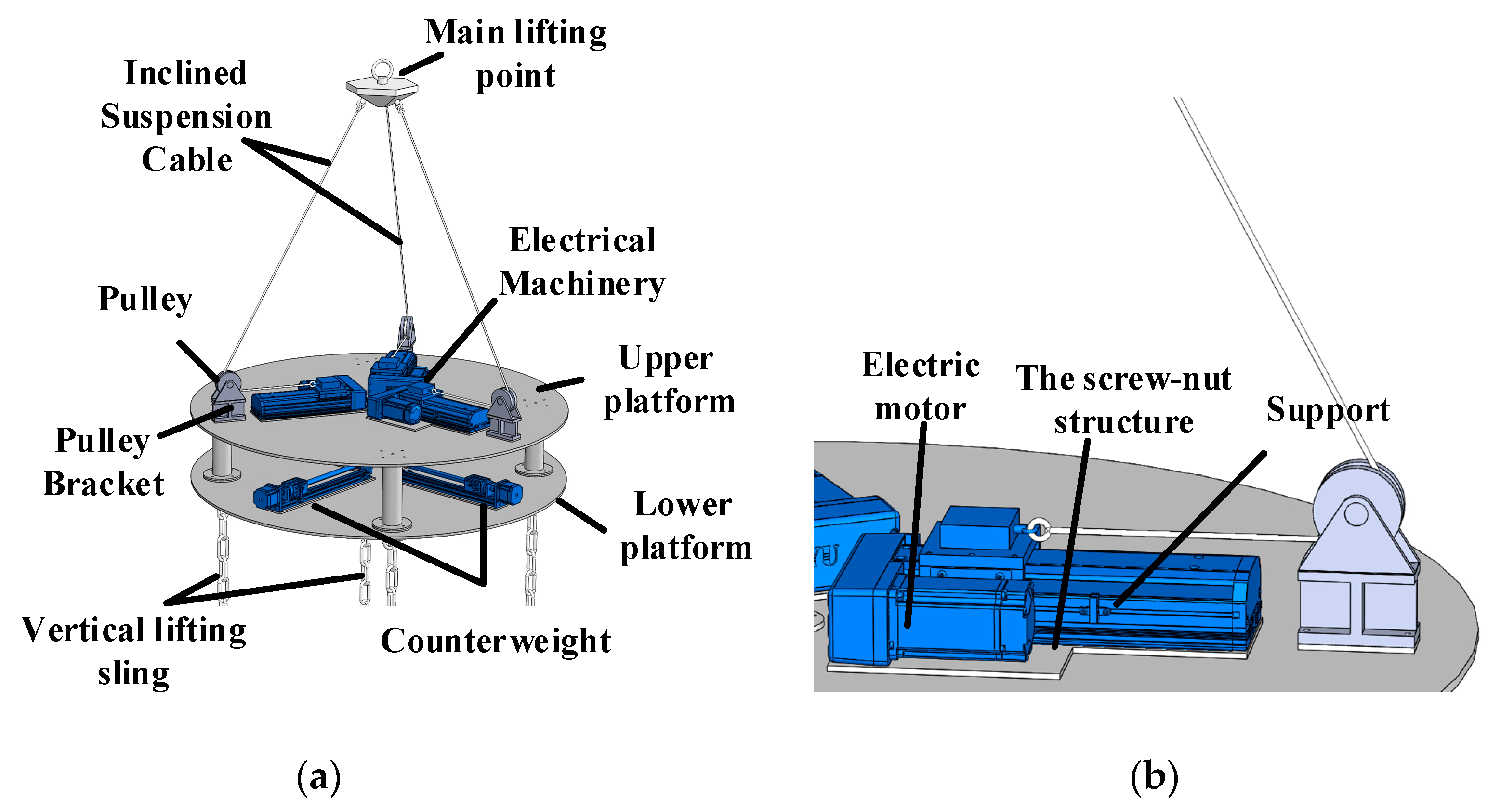
Figure 2.
Structure and force schematic of the automatic leveling robot. (a) Automatic leveling robot - structure schematic; (b) Counterweight structure schematic; (c) Schematic representation of the pulley structure; (d) Elevation schematic.
Figure 2.
Structure and force schematic of the automatic leveling robot. (a) Automatic leveling robot - structure schematic; (b) Counterweight structure schematic; (c) Schematic representation of the pulley structure; (d) Elevation schematic.
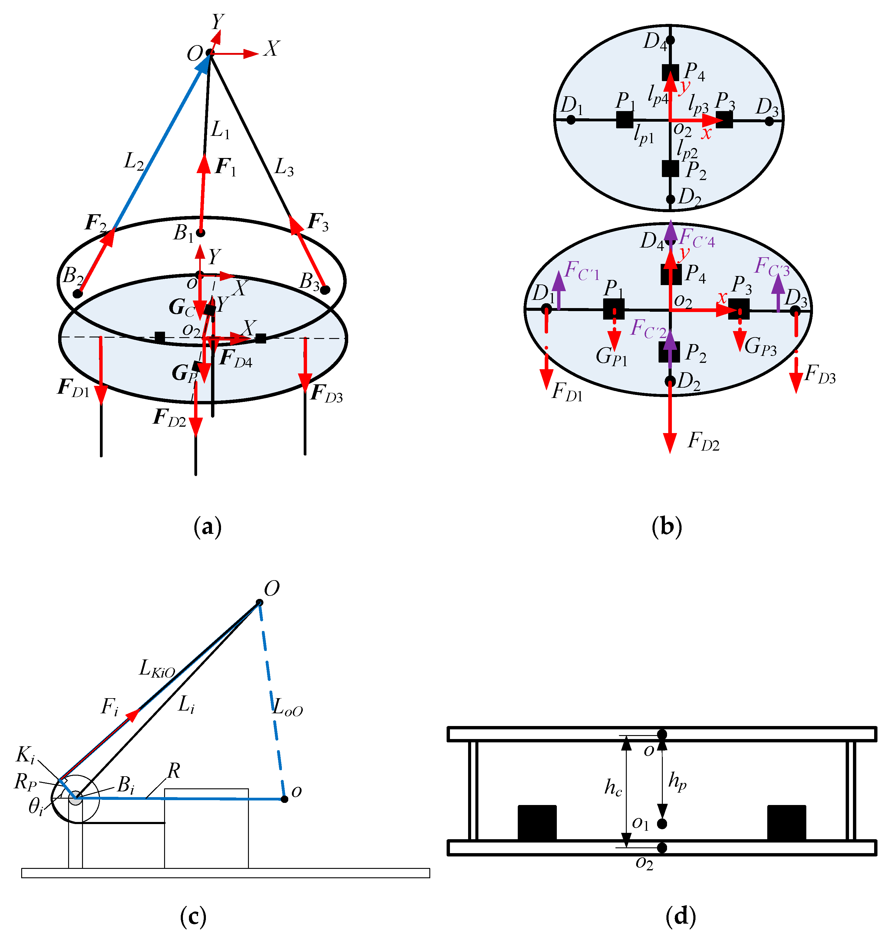
Figure 3.
Optimal cable adjustment scheme. (a) Adjusting L1, L2; (b) Adjusting L1, L3; (c) Adjusting L2, L3; (d) Adjusting L1; (e) Adjusting L2; (f) Adjusting L3.
Figure 3.
Optimal cable adjustment scheme. (a) Adjusting L1, L2; (b) Adjusting L1, L3; (c) Adjusting L2, L3; (d) Adjusting L1; (e) Adjusting L2; (f) Adjusting L3.
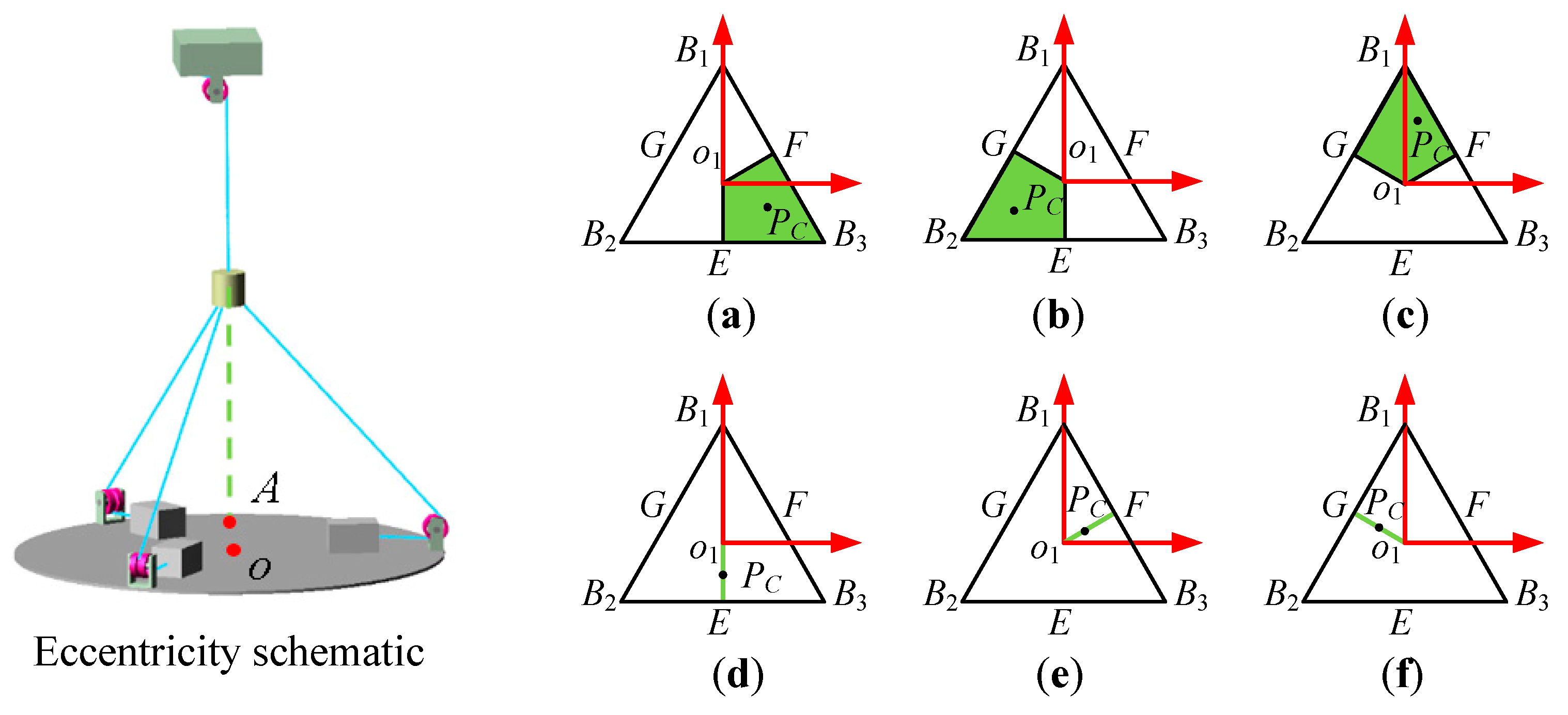
Figure 4.
Cable leveling state diagram. (a) Before starting; (b) Hoisting; (c) First leveling; (d) Second leveling; (e) Counterweight leveling.
Figure 4.
Cable leveling state diagram. (a) Before starting; (b) Hoisting; (c) First leveling; (d) Second leveling; (e) Counterweight leveling.
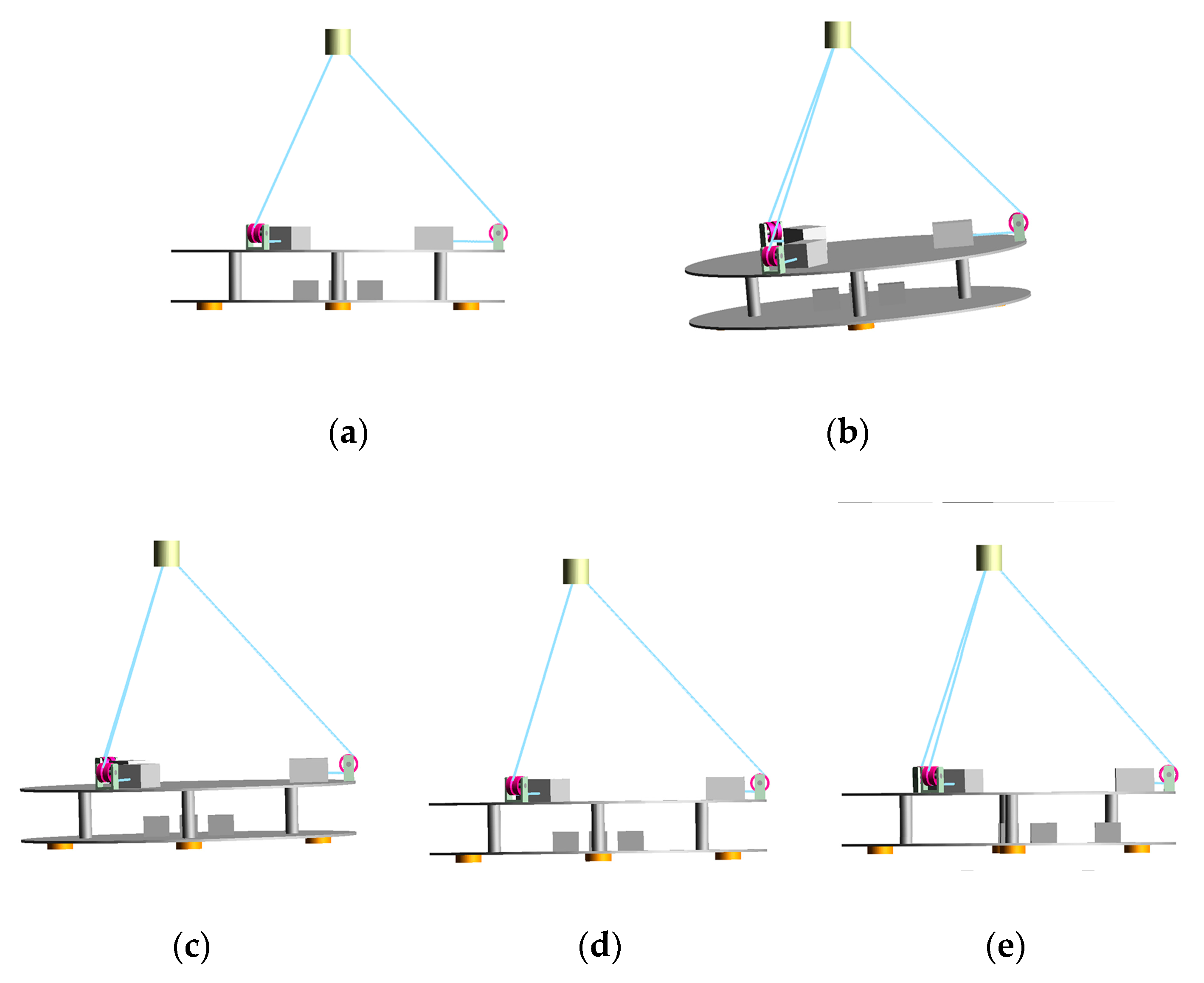
Figure 5.
Simulation results. (a) Inclination angles; (b) Cable lengths Li; (c) Cable forces Fi.
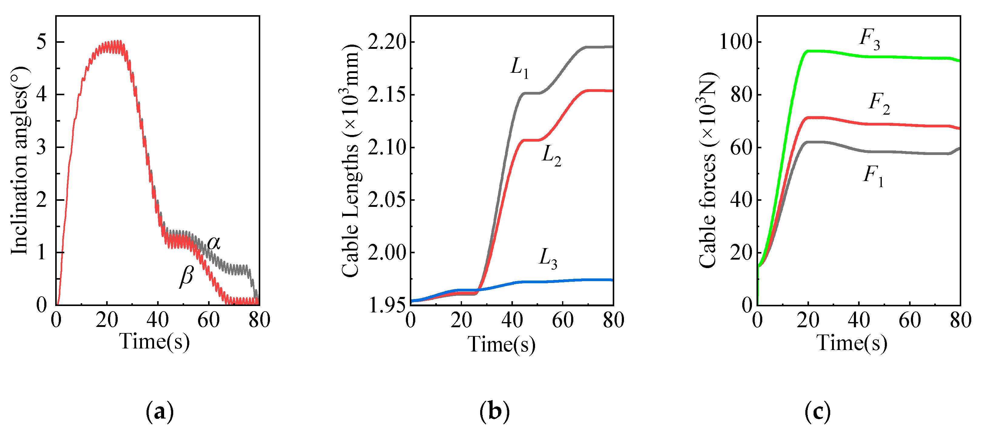
Figure 6.
Force and relative error during the external force loading process. (a) the variation of cable forces; (b) the relative errors between analytical solutions and simulation solutions.
Figure 6.
Force and relative error during the external force loading process. (a) the variation of cable forces; (b) the relative errors between analytical solutions and simulation solutions.
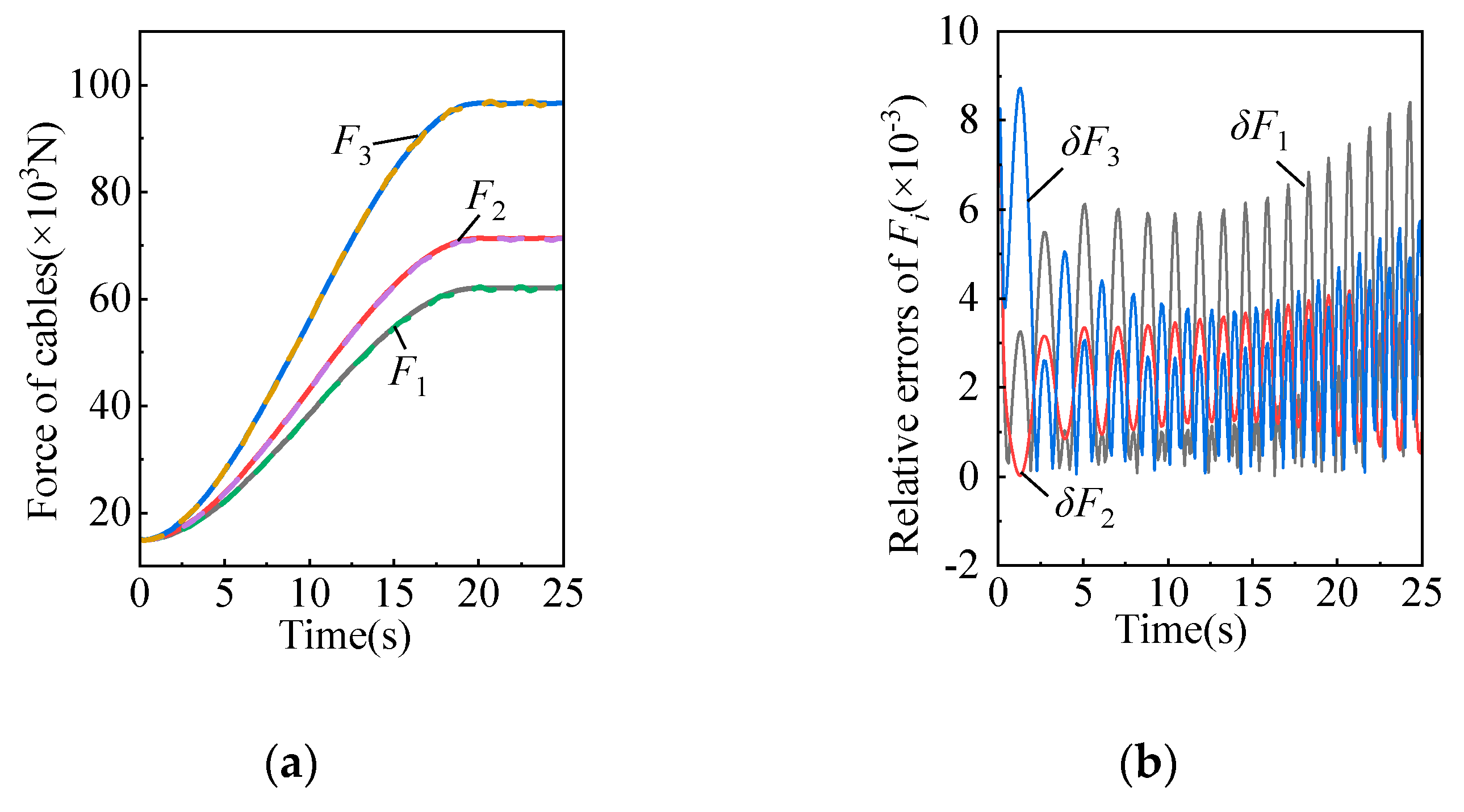
Figure 7.
Cable-driven parallel mechanism prototype model.
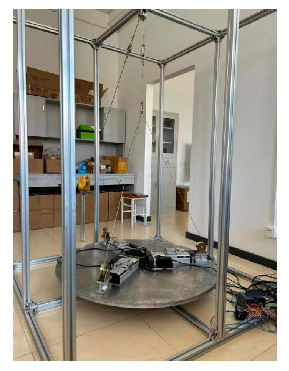
Figure 8.
Experimental model (a) Experimental model of situation a; (b) Posture of the moving platform after adjustment.
Figure 8.
Experimental model (a) Experimental model of situation a; (b) Posture of the moving platform after adjustment.
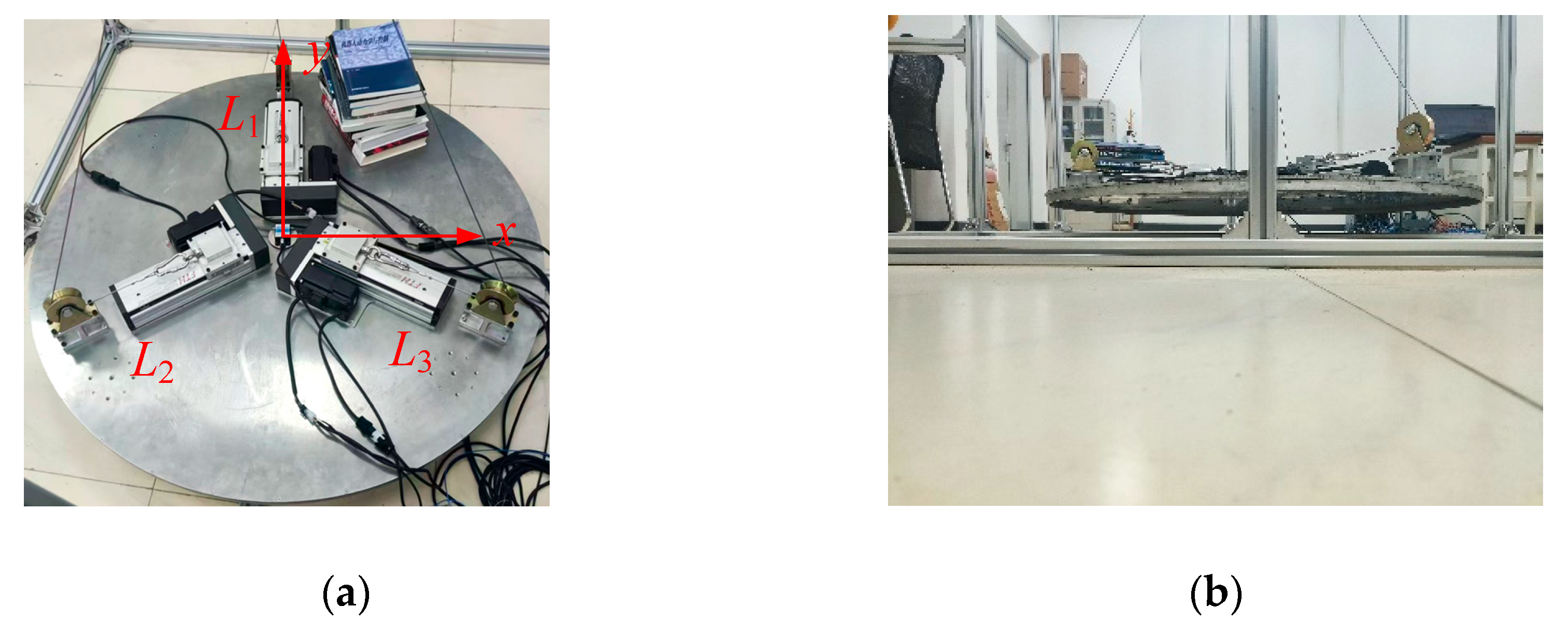
Figure 9.
Experimental result (a) The angle values of the inclination sensor before filtering; (b) The angle values of the inclination sensor after filtering; (c) Cable lengths.
Figure 9.
Experimental result (a) The angle values of the inclination sensor before filtering; (b) The angle values of the inclination sensor after filtering; (c) Cable lengths.
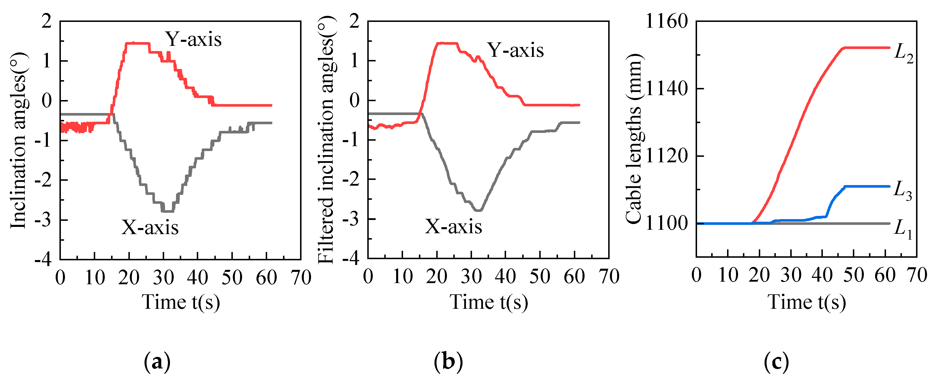
Figure 10.
Experimental model (a) Experimental model of situation b; (b) Posture of the moving platform after adjustment.
Figure 10.
Experimental model (a) Experimental model of situation b; (b) Posture of the moving platform after adjustment.
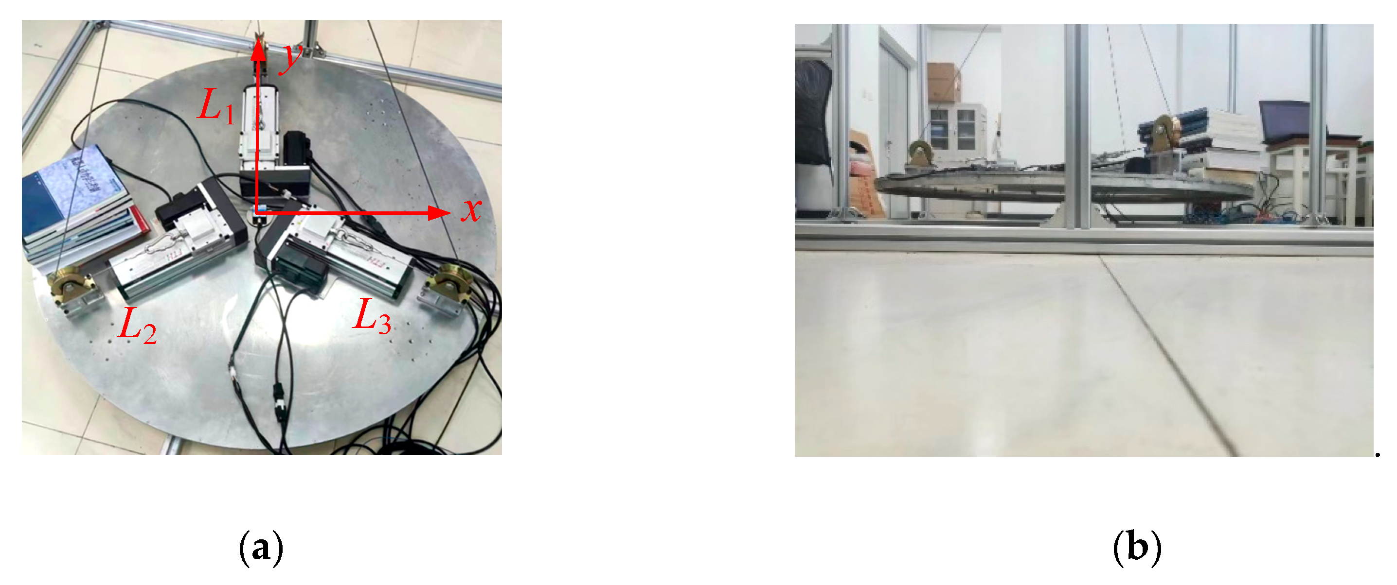
Figure 13.
Experimental result (a) The inclination angles before filtering; (b) The inclination angles after filtering; (c) Position of the counterweight.
Figure 13.
Experimental result (a) The inclination angles before filtering; (b) The inclination angles after filtering; (c) Position of the counterweight.
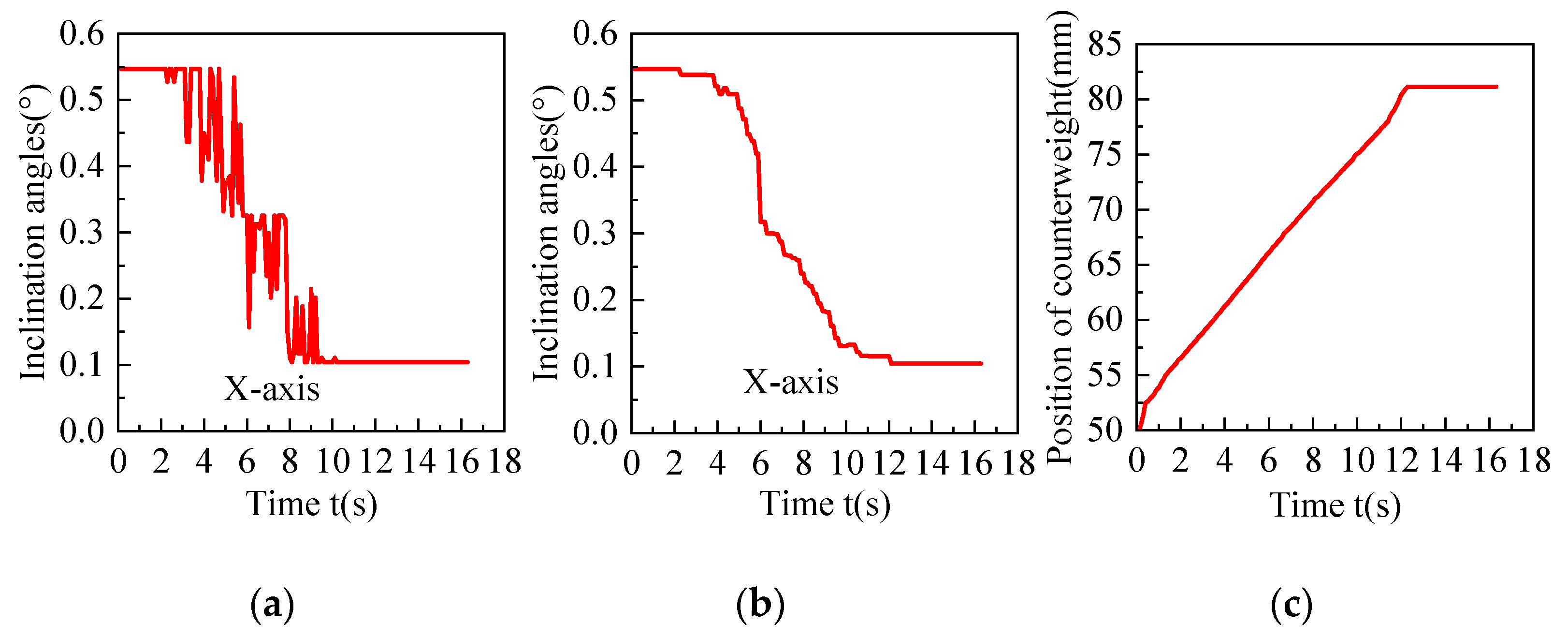
Figure 14.
Experimental result (a) The inclination angles before filtering; (b) The inclination angles after filtering; (c) Position of the counterweight.
Figure 14.
Experimental result (a) The inclination angles before filtering; (b) The inclination angles after filtering; (c) Position of the counterweight.
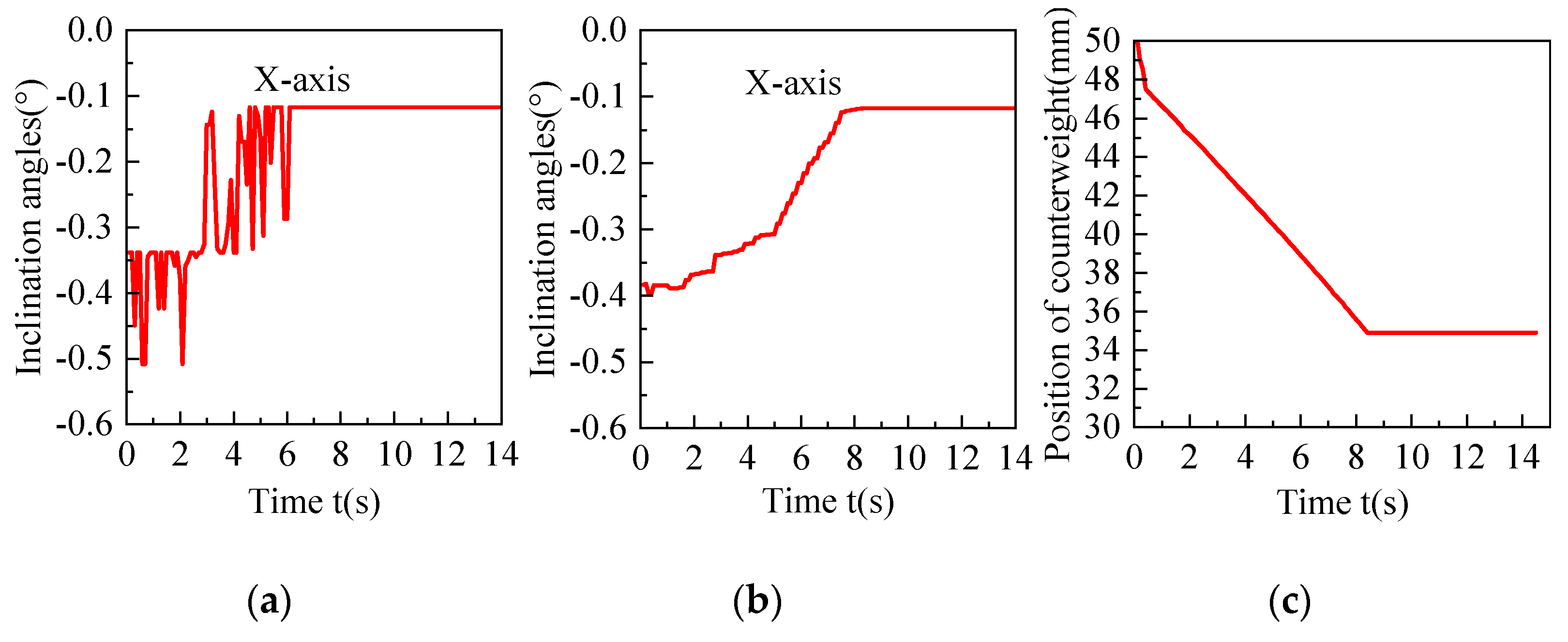

Table 1.
Given structural parameters and working load.
| Symbols | Value,Units | Symbols | Value, Units |
|---|---|---|---|
| lBio(R) | 1250 mm | FD1, FD4 | 20 KN |
| Rd | 1000 mm | FD2, FD3 | 50 KN |
| Rp | 68 mm | m1 | 831.5 kg |
| hc | 573.24 mm | m2 | 926.95 kg |
| hp | 428.9 mm | Mp | 400 kg |
| lpx0, lpy0 | 250 mm | Cable Initial Length L10, L20, L30 |
1956.4 mm |
Table 2.
Position of counterweight.
| Counterweight initial position /mm | Counterweight adjusted position /mm | Actual Adjustment Value /mm | |
|---|---|---|---|
| lp1、lp3 | -10.8 | -35.8 | -25 |
| lp2、lp4 | 9.3 | 522 | 512.7 |
Table 3.
The posture of the moving platform during adjustment.
| Counterweight initial position /mm | Counterweight adjusted position /mm | Actual Adjustment Value /mm | |
|---|---|---|---|
| lp1、lp3 | -10.8 | -35.8 | -25 |
| lp2、lp4 | 9.3 | 522 | 512.7 |
Disclaimer/Publisher’s Note: The statements, opinions and data contained in all publications are solely those of the individual author(s) and contributor(s) and not of MDPI and/or the editor(s). MDPI and/or the editor(s) disclaim responsibility for any injury to people or property resulting from any ideas, methods, instructions or products referred to in the content. |
© 2025 by the authors. Licensee MDPI, Basel, Switzerland. This article is an open access article distributed under the terms and conditions of the Creative Commons Attribution (CC BY) license (http://creativecommons.org/licenses/by/4.0/).
Copyright: This open access article is published under a Creative Commons CC BY 4.0 license, which permit the free download, distribution, and reuse, provided that the author and preprint are cited in any reuse.


