Submitted:
05 May 2025
Posted:
05 May 2025
You are already at the latest version
Abstract
Electric vehicles are transforming urban and metropolitan transportation, providing significant benefits to both the environment and society. However, the integration of electric vehicles necessitates a well-planned infrastructure, including a sufficient number of charging stations distributed at the local level, policies that encourage the purchase and operation of electric vehicles, and active participation of local governments and the automotive industry. Investments in improved car technologies, as well as renewable energy sources, will be critical in the shift to more sustainable metropolitan regions that have reduced pollution. Computer simulation based on virtual models performs an important role in the optimization of urban and metropolitan traffic by allowing rapid prototyping of real vehicle models, as well as the implementation of a wide range of test scenarios in real time. Assisted driving functions are critical in adjusting optimal driving behaviors to each of the particular scenarios of urban and metropolitan traffic. The situations discussed in the study were derived from real-world traffic and implemented and simulated on virtual models in the IPG CarMaker application. To calibrate electricity consumption in each of the metropolitan area's sectors, driving cycles have been embedded in the virtual model. These were allocated to component sectors based on the average travel speed and its variation.
Keywords:
electric vehicle
; real traffic
; virtual vehicle model
; computer simulation
; sustainability
; driving cycles
1. Introduction
Electric vehicles are an innovative and environmentally friendly alternative for urban and metropolitan transportation, contributing to the reduction of pollution, noise, maintenance and operating expenses while enhancing energy efficiency.
Electric vehicles are becoming increasingly prevalent in urban and metropolitan traffic because of their ecological, economic, and technological advantages, providing considerable benefits to congested urban areas while also posing issues that necessitate careful planning and management.
- Reduced atmospheric pollution because electric vehicles do not generate polluting contaminants: carbon monoxide (CO), nitrogen oxides (NOx), particulate matter (PM), respectively greenhouse gases (GHG);
- Noise pollution is reduced as a result of the quietness of electric motors and systems used in electric vehicles;
- Operating costs are reduced due to the excellent energy efficiency of the electric motors that equip electric vehicles, and respectively due to the low price of electricity (particularly energy from renewable sources) compared to the price of fossil fuels;
- Maintenance costs are lowered since the systems that equip electric vehicles are less complex;
- Access to restricted areas in historic urban centers, free parking, and public and/or private charging stations with preferential pricing for power;
- Reductions on taxes and assessments, as well as financial incentives to buy new electric vehicles.
- Infrastructural development in the majority of major cities, reduced number of public and private charging stations that may be insufficient to serve all electric vehicles;
- Increase in electricity consumption in national grids (at certain times of the day) as the number of electric vehicles grows;
- In comparison to vehicles equipped with conventional propulsion systems (internal combustion engines and hybrid propulsion systems), autonomy is limited;
- In comparison to vehicles powered by conventional or hydrogen fuel, there is a higher rate of refueling, which may be expensive for users;
- The initial cost was higher than conventional vehicles in similar categories;
- Environmental issues arising from the recycling of batteries, as well as the management of waste batteries.
The future of electric vehicles in urban and metropolitan traffic is dependent on the adoption and implementation of favorable government policies based on subsidies and fiscal incentives for the purchase of these vehicles, as well as restrictions and prohibitions imposed on polluting vehicles in metropolitan areas.
In addition, advanced and innovative technologies used in the automotive industry, such as battery production technologies, fuel cell systems, and so on, will have a significant impact on the transition from conventional to electric vehicles.
Adopting electric vehicles in urban and metropolitan traffic represents a critical step toward the development of sustainable metropolises, which require a mobility solution that, in addition to the benefits of environmentally friendly transportation with zero local emissions (ZLE), provides the possibility of traffic decongestion through the integration of mobility services such as car-sharing and/or ride-hailing.
The implementation of Artificial Intelligence AI-based algorithms, such as the Tabu Search Algorithm, which employs Particle Swarm Optimization [6,7], has resulted in the efficient optimization of urban and metropolitan routes for electric vehicles, as demonstrated in real-world logistical scenarios.
Ran et al. [8] introduced an automated type of clustering algorithm K-means that incorporates the noise algorithm, Genetic Algorithm (GA), an Adaptive Fuzzy System (AFS), and the Ant Colony Optimization (ACO) algorithm, in addition to the algorithm for tracking global GPS (Global Positioning System) positions and optimizing urban vehicle traffic. The primary goal of the K-means algorithm is to identify economically feasible and spatially homogenous metropolitan areas for traffic routing. The optimal routes for vehicle movement are obtained by controlling traffic based on GPS location information of a maximum number of vehicles in traffic, or by managing traffic in intersections [9].
Mirjalili et al. [10] proposed the metaheuristic Grey Wolf Optimizer (GWO) algorithm based on a dynamic mobility scenario inspired by nature, with floating options classified at the hierarchical level in making decisions about the fixed route, in order to provide quick and precise solutions to various traffic scenarios. GWO is a hybrid optimization algorithm that uses Machine Learning (ML) methods based on the implementation of an Artificial Neuronal Network (ANN) [11], which uses information provided and shared by all participants in the traffic [12].
The Fast Firefly Algorithm (FFA) was introduced to address the difficult problem of solving Nondeterministic Polynomial (NP) time hardness using non-convex functions with equality and inequality constraints [13]. The algorithm employs a search based on a large number of solutions that provide base information, allowing the algorithm's mechanism to facilitate a good learning for training the parameters required to make decisions in a distributed way to balance exploration and exploitation. Bazi et al. [14] proposed a fast FFA for reducing search space by randomly selecting a significant group of subjects in motion to cover the whole search space under consideration.
Artificial Bee Colony (ABC) [15] is an algorithm based on a solution to an optimization issue in identifying resources where the number of subjects considered is equal to the number of solutions. Each topic under consideration is involved in the search process and ranks the best resources discovered. At the end of the search process, subjects share information on the position of memorated resources. In the field of mobility, the proposed algorithm provides routes that combine reduced travel time with the selection of optimal travel distances, while managing participant interference through continuous communication [16].
In their work, the authors implemented the results of their studies based on some of the algorithms presented earlier in the virtual model developed in CarMaker using command and control tools such as IPGRoad, IPGDriver, Traffic, Environment etc.
2. Materials and Methods
2.1. Simulation Platform
Computer simulation is used to simulate real-world studies in a virtual environment, using a theoretical model that represents a digital image of an existing physical model, and the process of computer simulation is used to develop and improve the quality of this model. The complexity of the virtual model must correspond to the reality of the evaluated model, as complicated as necessary but as simple as possible, so that the results obtained from computer simulations can be validated by experimental results [17].
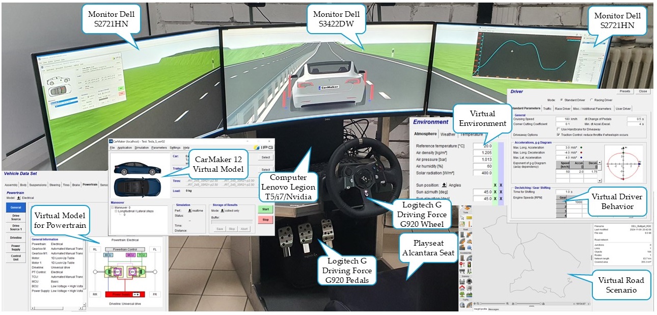
CarMaker (https://www.ipg-automotive.com/) is a simulation platform used by a large number of automotive companies to create, test, and optimize virtual vehicle models in various architectural designs [18,19]. There are virtual vehicle models in the application library that contain predefined parameters of the real vehicle, such as dimensions, mass, aerodynamics, steering and suspension systems, engine characteristics, and driver assistance functions ADAS (Advanced Driver-Assistance System) (Figure 1).
According to [20], CarMaker is a versatile platform that allows the development and real-time simulation of electric vehicles integrated into a virtual environment capable of simulating a variety of external factors such as meteorological conditions, various traffic scenarios, different driving behaviors for the virtual driver, the ability to define any type of vehicle, and the digitization of any sector of Google Earth/Map etc. [21].
Realistic scenarios that may be defined in CarMaker allow for the assisted driving of virtual models using ADAS systems, which are connected via V2X (Vehicle-to-Everything) systems between vehicles and the intelligent environment.
Toth et al. [22] used measurements taken from real-world vehicle movements to create a simulation model that ensures compatibility with the real-world model for each driving scenario chosen.
Another advantage of CarMaker's virtual models is that they allow for real-time testing of sophisticated HiL (Hardware-in-the-Loop) systems [23], as well as the selection of simulated CAN parameters.
CarMaker platform has obtained ISO 26262 certification from TÜV Nord [24] for developing complex simulation solutions and validating virtual vehicle models, which is an important factor in the credibility of scientific research results based on simulation scenarios.
2.2. Selection of the Initial Data
2.2.1. Electric Vehicle Characteristics and Performance
A Tesla Model 3 was used to perform tests and collect data on electric energy consumption and recovery in the metropolitan area in consideration. This vehicle model was used to create a virtual model, which is utilized in computer simulations.
2.3. Virtual Model Development
2.3.1. Virtual Model for Electric Vehicle
The virtual model for the electric vehicle Tesla Model 3 was created in CarMaker (Figure 2) [29] using data extracted from the real model's structural characteristics in addition to experimental determinations performed with the vehicle.
Computer simulations allow for high-precision results at a low cost, provided that the virtual model is validated through experimental determinations [30,31,32].
The torque/power characteristic (Figure 3) [33] indicates that the electric motors of the Tesla Model 3 operate at a constant torque, where the active power increases linearly as the torque increases, and at a constant power, where the torque changes in opposite relation to the torque of the motor. Power and moment characteristics of electric motors that will be determined in the development of a virtual vehicle model are constant torque, which indicates the maximum motor speed limited by the maximum current admissible, constant power, which indicates the maximum motor speed, and the maximum motor power, which decrease due to mechanical limitations [34].
The motor torque MEM is calculated using the following equation:
where MMax(ω) is the maximum motor torque for the electric motor/generator, and LoadEM is the electric motor's load characteristic.
The power of an electric motor in the motor mode PElecMot and in the generator mode PElecGen is calculated using the following equations:
where ηMot represents motor efficiency and ηGen represents generator efficiency.
The battery modelled in CarMaker represents the vehicle's power supply PS and is part of the powertrain group. Batteries contain all low voltage LV and high voltage HV electric components (HV1 for the construction variant with one electric motor and HV1+HV2 for the construction variation with two electric motors) as well as the corresponding electrical circuits (Figure 4).
The command and control of the powertrain group is performed by the PTControl module, which manages the characteristics of each electronic control unit (ECU), which manages the vehicle's operating regime (Figure 5), as follows [35]:
- Stabilizing the vehicle's operational status by activating the start/stop button;
- Interpretation of load pedal position for determining desired torque for an electric motor;
- Mechanical energy management based on strategy mode selection;
- Electric energy management for controlling battery State-of-Charge (SoC) and Depth-of-Discharge (DoD);
- Estimate the maximum torque of the electric generator at each rotation;
- Calculate the maximum quantity of energy used to power HV electric motors and other LV electric consumers in the vehicle's system.
The electric energy flux from batteries to electric consumers is modelled using power consumption equations, which are generated by high-tension consumers PHV and low-tension consumers PLV [35].
where PAuxHV and PAuxLV represent the power consumed by electric auxiliary devices, PMotorHV and PMotorLV represent the power generated by each electric motor in the vehicle's architecture, PHVtoLV represents the power consumed by the DC-DC converter, and ηDC-DC represents the DC-DC converter's voltage.
2.3.2. Virtual Model for Simulation Cycle
Considering driving cycles that were selected for computer simulations were implemented and validated in the CarMaker application developed by the company IPG Automotive [36]. These are part of the manufacturer's validated element library (IPG Automotive) and are available to licensed users.
- The WLTC (Worldwide harmonized Light vehicle Test Cycles) are part of global testing procedures for light automobiles. The WLTP (Worldwide harmonized Light vehicle Test Procedure) has provisions specifically for testing electric vehicles classified as class 3 [37];
- The FTP-75 (Federal Test Procedure) is part of the EPA-UDDS (Environmental Protection Agency urban dynamometer driving schedule) testing procedures. In the United States, FTP is used to evaluate the performance of light-duty cars [38];
- The HWFET (Highway Fuel Economy Test) is part of the EPA testing procedures and is used to assess the performance of light vehicles on high-speed roads, specifically highways [39];
- The ARTEMIS urban cycle is part of the European ARTEMIS project (Assessment and Reliability of Transport Emission Models and Inventory Systems), which is based on statistical analysis of a database of real-world traffic models [40];
- The JC08 (Japanese Cycle) is one of the Japanese procedures for testing the performance of light vehicles in urban traffic, which includes periods of stoppage, frequent acceleration and deceleration [41];
- The NYCC (New York City Cycle) is one of the EPA's procedures for testing the performance of light vehicles in heavy traffic environments in urban and metropolitan areas [42].
2.3.3. Virtual Road for Metropolitan Area
The selected route to perform computer simulations was created in CarMaker/IPGRoad (Figure 7), starting with the route used for experimental determinations with the Tesla Model 3. This route covers the metropolitan area of Cluj, Romania, on one of the most heavily trafficked sections of the main road, including the center area on the west axis and the ring road for accessing the industrial zone from the north to the south via the Transylvania Highway [44].
Similar to the case presented, Magosi et al. in [45] developed virtual models for roads used in computer simulations, with an infrastructure consisting of the following elements: traffic lights, traffic lines, road markings, borders, barriers, traffic signs, public lighting, and more.
2.3.4. Virtual Environment
The detailed description of the environment allows for the smallest possible difference between the real scene and the virtual reality. Thorat et al. used the virtual environment model in [46], which was developed based on a virtual road model, an infrastructure model, and a weather model. The model in discussion is based on real-world road maps that have been digitized using geographic coordinates from Google Maps. For a photorealistic visualization of 3D scenes, the authors used CarMaker/Movie NX. This equipment uses physical rendering through 3D processing to ensure a combination of realistic illumination and meteorological effects appropriate for each simulation scenario [47].
Meteorological conditions were established in the CarMaker/Virtual Environment utility for computer simulations using data from the Raspisaniye Pogodi meteorological station (https://rp5.ru/) [48], which provides real-time data, including a meteorological archive with complete data records from recent years. The extra time interval (date/time) from the meteorological archive was corresponding to the displacement in real traffic conditions with the Tesla Model 3 on the road considered for the acquisition of experimental data.
The mathematical model for the environment is defined based on equations that specify air temperature, air pressure, air density, and sound speed [35]. The air temperature in the ambient environment is calculated using the following equation:
where T0 is the temperature for height above mean sea level zero, Telev is the temperature compensation factor based on elevation, TsRoad is the temperature compensation factor based on road coordinates, and Ttime is the temperature compensation factor based on time of day.
The temperature of the air as a function of elevation is calculated using the equation:
where Δh is the difference in height above mean sea level, and Celev is the temperature decrease coefficient.
The ambient air pressure is calculated using the following equation:
where p0 is the pressure for height above mean sea level zero.
The density of air in the ambient environment is calculated using the following equation:
where Rs is the specific gas constant.
The speed of sound in the air is calculated using the following equation:
where, k is the air's heat capacity ratio.
2.3.5. Virtual Driver Behavior
The ideal virtual driver behavior for computer simulations is based on Tesla's Autopilot features [29].
The evaluated Tesla Model 3 is equipped with Autopilot hardware [25], which assists the driver and provides intuitive access to travel information, with the driver in charge of controlling the vehicle's movement. According to SAE J3016™ [49], Tesla's Autopilot system is classified as LEVEL 2TM (partial automation) [50], with the driver's role being to assist with dynamic driving tasks (DDT) during critical situations. Driving is continuously monitored, with the driver's gaze fixed on the road (eyes on), and the driver's hands can be temporarily removed from the wheel of the vehicle (hands temp off) [51].
The Autopilot system, based on the information provided by the video camera set, which is equipped with a real-world vehicle model and radar sensors to match up with the virtual vehicle model, provides the following ADAS driving assistance functions [52]:
- Traffic-Aware Cruise Control is a function that allows for adaptive cruise control in response to vehicles in front of it;
- Autosteer is a function that allows for the maintaining of traffic lanes and the direction of movement while steering;
- Auto Lane Change - a function that allows for the automatic change of a vehicle's lane using a direction indicator (on turn signal);
- Navigate on Autopilot - a feature that allows the following of a predetermined route based on GPS coordinates;
- Autopark - function that allows parking parallel or perpendicular to the roadside;
- Actually Smart Summon is a function that allows the vehicle to be moved from its parking spot to the location where the driver has summoned it by a maximum of 6 meters.
All these functions were defined and configured throughout the virtual model's development using the CarMaker/IPGDriver application [36].
Endsley [52] determined that after traveling over 4300 kilometers during a six-month period in a Tesla vehicle with the mentioned assistance functions, at least one of these functions was activated in 84% of the trips.
Simulating command and control actions of a real-world driver in IPGDriver is accomplished by providing input parameter values, calculating a response based on the virtual model's operating algorithm, and transmitting output parameter values to the virtual propulsion and direction system (Figure 8) [36].
Camera sensors that incorporate both the virtual and real models for the Tesla Model 3 are positioned to provide a circular image of the surrounding environment and belong under the category of Hi-Fi virtual sensors. Camera sensors filter sent information and add data about physical effects that occur in the real world, particularly in terms of object detection and classification. Camera sensor characteristics include the ability to detect visible objects for the sensor, estimate distances to visible objects, and calculate the height of objects (occlusion calculation) [35].
The detection of objects in close proximity is dependent on the environment parameters RainRate and VisRangeInFog. The visibility αEnv camera sensor is calculated using the following equation:
Where RainRatemax and VisRangemax are maximum values for environmental parameters.
Distance estimation DistEst to visible objects is calculated using the following equation:
where Dist is the actual distance to the object, f is the camera's focal length, b is the baseline, and DistErr is the disparity error.
The radar sensor that is equiped on the virtual model for the Tesla Model 3 corresponds to the RSI (raw signal interface) sensor category, which provides raw information and functions similarly to real sensors. The CarMaker simulation application collects, filters, and interprets information transmitted by RSI Radar sensors, which complements the virtual model.
Radar sensor detection characteristics are based on the signal-to-noise ratio (SNR), taking into account the following: detection threshold, antenna gain characteristics, transverse radar cross sections of detected objects RCS (radar cross section), propagation characteristics in relation to atmospheric conditions, and object occlusion [35].
The minimum detection threshold (SNRmin) is calculated using the equation:
Where PFA represents the probability of a false alarm, whereas PDmin is the least probability of detection.
The intensity of the received signal SS is calculated using the following equation:
where, PRadar is transmitted power, GAnt is antenna gain, λ is wavelength, RCS is radar cross section, r is the distance between the radar sensor and the monitored object, LA are extra system losses, and LAtm are atmospheric losses.
The antenna gain is calculated based on the antenna direction (x, y, z) and the elevation θ and azimuth φ parameters, according to the equation:
where parameters a and b represent the primary lobe of the aperture dimensions.
Transversal RCS thresholds for objects within close proximity are determined by radar sensor resolution, object size, direction of incidence, object occlusion, and object merging (Figure 9).
The Autopilot functions that equip the Tesla Model 3 have been implemented in the virtual model via the Vehicle Control module, where there are two models of autonomous driving functions: GLxC (generic longitudinal control) for vehicle movement (Table 4), and GLyC (generic lateral control) for vehicle direction (Table 5).
Trajectory planner (TP) for virtual model movement has been implemented based on a set of established rules for planned routes with well-defined boundaries. The rule set can determine whether the vehicle remains on the current travel lane or should the vehicle's changing lanes. A travel scenario assumes that the virtual vehicle model is placed in the middle of the right-hand lane. If a slower vehicle moves in front of the virtual model, preventing it from reaching stable cruising speed, and the lane on the left is free, a Bézier curve is planned to change the lane of circulation [53].
2.3.6. Virtual Traffic Model
The virtual traffic model includes a set of maneuvers to move traffic-related movable objects. Each maneuver consists of a longitudinal and a lateral component [29].
To simulate a random/stochastic traffic model for urban and metropolitan areas, the following scenarios were generated: static vehicles, slow-driving vehicles, fast-driving vehicles, vehicles that abruptly change lanes, vehicles that coincide at a crossing, bicycle riders, and pedestrians crossing the road [20].
Noei et al. [54] used CarMaker simulation tools to evaluate vehicle tracking behaviors, change driving lane, and adapt movement for simulation of driving scenarios in a generated traffic environment. As a result, the virtual traffic model includes ten different types of drivers (from conservative to aggressive), ten different vehicle models, various driving scenarios, potentially dangerous interventions from other traffic participants, and other unknown situations.
The virtual traffic model was considered for governing computer-generated road simulations implemented in CarMaker/Road. In the computer simulations for which the cycles of movement described in section 2.3.2 "Virtual model for simulation cycle" were implemented, the virtual traffic model was not used, instead being replaced by procedures for controlling the driving cycles (acceleration/deceleration).
2.4. Driver-in-the-Loop Simulator
2.4.1. Simulator Development
Driving simulators based on virtual vehicle models have been used in studies and by other research groups. As a result, Kwon et al. [55] used a compact driving simulator that included real-world vehicle components to assess driving behaviors for different drivers in laboratory conditions.
Aparow et al. [56] used a driver-in-the-simulation platform to verify and validate the simulation model developed in Matlab Simulink and IPG CarMaker based on various test scenarios, defined with real traffic data.
The virtual scenarios described in previous chapters have been implemented in a simulator built on the Driver-in-the-Loop simulator concept (Figure 10) [57,58,59], which is used to run computerized simulations based on real-world scenarios traveled by the Tesla Model 3 on the selected road.
CarMaker/CockpitPackage extension permits controlling the movement of a virtual vehicle using an external control device, which in our case is a Logitech G Driving Force G920 Wheel [20].
The CockpitPackage software architecture is based on a multiplatform development library called SDL2 (simple direct-media layer), and simulator input signals are divided into two categories:
- Axis Events indicate the evolution of movement on coordinate axis, which are analogic values generated by the steering wheel and/or pedal actions.;
- Button Events are actions that correspond to "true" or "false" values for certain predetermined selections, like light blocks, signalization, and sound alerts.
2.4.2. Simulation Task
Using the virtual Tesla Model 3 model, computer simulations were run for the following tasks under similar environmental and traffic conditions to those used for experimental data collection in the considered metropolitan area:
- In CarMaker with the plug-in Cockpit Package Standard, a human driver used a virtual Tesla Model 3 to simulate real-world driving conditions using a Driver-in-the-Loop simulator. The following parameters were monitored and recorded using CarMaker/IPGControl: Car.Distance (m), Speed (km/h), consumption, respective recovery of electric energy PT.BattHV.Energy (kWh), and the key parameters of SoC battery charging PT.BCU.BattHV.SOC (%).
- ADAS functions (according to Level 2 SAE 3016TM) [60] ran computer simulations using a virtual Tesla Model 3 model similar to real driving conditions, ensuring movement control through the CarMaker/IPGDriver utility in standard driver mode in accordance with the values of the parameters corresponding to the behavioral profile of the virtual driver presented in Table 6, respectively in extended driver mode in accordance with the values of the parameters corresponding to the behavioral profile of the virtual driver presented in Table 7.
The integration of real-world driving scenarios into a digital world of computer simulations is a critical step in the research and development of modern vehicles. To implement these scenarios as accurately as possible, various vehicle driving cycles have been used, which reflect the behavior of a driver in a variety of driving situations, such as variable traffic, urban, and extra-urban [61].
3. Results
3.1. Experimental Results
The route selected for a journey with a Tesla Model 3 in the Cluj metropolitan area, has been divided into sections based on the city of Cluj-Napoca's zonal boundaries. The route is divided into five main segments, with each sector considered in the order in which for the vehicle was driven for the experimental data collection.
The experimental results were derived from real-world consumption graphs of the Tesla Model 3 and include information on the length of the road, the average speed of movement in each sector, the amount of energy consumed by the vehicle, and the amount of energy recovered through energy recovery (Table 8).
The experimental results obtained after completing a selected real-world route in the metropolitan area have been utilized as a reference value in validating computer simulations with a virtual model for Tesla Model 3.
CarMaker/Environment and CarMaker/Load utilities were used to configure the medium and load parameters of the virtual model to make them similar to real-world conditions.
3.2. Simulation Results
All experimental data collected after completing the selected route in the Cluj metropolitan area was compared to the results obtained with the virtual Tesla Model 3 after running simulations in CarMaker on the Driver-in-the-Loop simulator for the metropolitan route (Table 9), respectively for selected and implemented driving cycles on the corresponding sectors based on driving cycles characteristics (Table 10).
The average speed (km/h) was calculated based on the distance traveled on each road sector and the time it needed to complete these sectors.
The energy consumption (kWh/km) in each sector is influenced by travel speed, the structure of the road, and traffic conditions. Because real traffic could not be implemented identically in the simulating process, in the initial conditions for defining simulating tasks, speed was maintained constantly for each sector and was considered to be the medium speed required to complete the sector.
The recovered energy (km/h) from regenerative braking was determined from the graphic recorded in the ECU unit of the Tesla Model 3 and was taken into consideration in computerized simulations of each road sector by defining some braking actions in the CarMaker/Maneuver tool.
As mentioned in section 2.3.6 "Virtual traffic model," for each of the sectors considered, one of the driving cycles available in the CarMaker library was chosen and implemented. The association of selected driving cycles to road sectors was accomplished by considering the vehicle's operational model and travel regime in relation to traffic characteristics, and by considering the respective speed limits for the sectors under consideration.
For urban zones (urban center, urban peripheral 1, urban peripheral 2), driving cycles like JC08, NYCC, and ARTEMIS were considered, which assume a low average travel speed with frequent acceleration and deceleration.
On routes from urban metropolitan zones (urban metropolitan, extra-urban metropolitan 1, and extra-urban metropolitan 2), which are generally located adjacent to major urban agglomerations and are crossed by national road with speed restrictions, universal driving cycles WLTC and FTP-75 have been selected.
The highway driving cycle (HWFET) has been chosen for sections of the metropolitan ring where traffic moves at a high speed in a relatively steady flow of vehicles.
To cover all types of driver behavior, computer simulations for each sector were evaluated with core sets in CarMaker/Driver for three characteristics of the driver behavior: normal driver behavior, aggressive driver behavior, and defensive driver behavior (Table 10).
Figure 11(a-f) displays the graphs for energy consumed and energy recovered for each of the driving cycles selected for the sectors under consideration.
The operating conditions for driving cycles (see Table 3) involve frequent and significant acceleration, which determines the consumption of additional electric energy from the electric motor to generate the necessary power for motion. The energy balance for total electric energy consumption E includes the quantity of energy consumed C during acceleration and the quantity of energy recovered R during deceleration.
where x represents the driving cycles , n represents the number of accelerations that determine the energy consumption, and m represents the number of decelerations that determine the energy recovery.
The recovery of energy in the graphs in Figure 11 is highlighted by a constant level, which can represent a growing trend in the evolution of energy consumption in the graph sections that follow a significant deceleration.
In circumstances in which the deceleration is excessive, mechanical braking is activated without the recovery of energy. Similarly, excessive acceleration increases the instantaneous power demand of the electric motor, resulting in a significant increase in electric energy consumption and a decrease in autonomy. Similarly, strong braking sequences reduces energy recovery efficiency, resulting in increased energy consumption and decreased autonomy [62].
4. Discussions
To evaluate electric energy consumption in driving scenarios considered in metropolitan areas, evaluations have been implemented in a virtual model simulating the six variants of driving cycles assimilate to sectors that have travel conditions similar to these driving cycles' characteristics (Figure 12).
Extra-urban metropolitan 1 (17.49% of total route) and extra-urban metropolitan 2 (10.41% of total travel) have been integrated into the WLTC driving cycle, which tests the performance of vehicles in circulation under all conditions. The total amount of energy consumption in this area was 3.008 kWh (32.27% of total energy consumption) for normal driving behavior, 3.216 kWh (29.50% of total energy consumption) for aggressive driving behavior, and 2.768 kWh (30.47% of total energy consumption) for defensive driving behavior. The total quantity of energy recovered in this area was 0.64 kWh (50.29% of total recovered energy) for normal driving behavior, 0 kWh (0% of total recovered energy) for aggressive driving behavior, and 0.08 kWh (15.26% of total recovered energy) for defensive driving behavior.
The metropolitan ring (34.91% of the total route) provides rapid transportation on the ring road with a medium to high speed (up to 80 km/h) has been integrated into the HWFET driving cycle, which tests the performance of vehicles on the highway driving conditions. The total quantity of energy consumed in this area was 3.32 kWh (35.62% of total energy consumption) for normal driving behavior, 3.46 kWh (31.77% of total energy consumption) for aggressive driving behavior, and 3.10 kWh (34.16% of total energy consumption) for defensive driving behavior. The total quantity of energy recovered in this area was 0.46 kWh (36.18% of total recovered energy) for normal driving behavior, 0 kWh (0% of total recovered energy) for aggressive driving behavior, and 0.36 kWh (68.77% of total recovered energy) for defensive driving behavior.
The FTP-75 cycle, which tests the performance of vehicles in circulation in all conditions of travel in the United States, has been incorporated into the urban metropolitan (17.85% of the total route), which ensures constant travel at a medium speed of up to 42 km/h. By implementing this driving cycle in an area near a extra-urban metropolitan area, a comparison of WLTC and FTP-75 results was performed. The total amount of energy consumed in this area was 1.65 kWh (17.79% of total energy consumption) for normal driving behavior, 1.73 kWh (15.87% of total energy consumption) for aggressive driving behavior, and 1.53 kWh (16.90% of total energy consumption) for defensive driving behavior. The total quantity of recovered energy in this area was 0.143 kWh (11.28% of total recovered energy) for normal driving behavior, 0 kWh (0% of total recovered energy) for aggressive driving behavior, and 0.06 kWh (11.72% of total recovered energy) for defensive driving behavior.
Urban peripheral 1 (5.83% of the total route) allows travel in variable traffic conditions to the periphery of the main city with a travel speed of up to 18 km/h. The ARTEMIS driving cycle, which tests the performance of vehicles in urban traffic, has been integrated. The total quantity of energy consumed in this area was 0.40 kWh (4.39% of total energy consumption) for normal driving behavior, 0.85 kWh (7.82% of total energy consumption) for aggressive driving behavior, and 0.54 kWh (5.97% of total energy consumption) for defensive driving behavior. The total quantity of energy recovered in this area was 0.009 kWh (0.78% of total recovered energy) for normal driving behavior, 0 kWh (0% of total recovered energy) for aggressive driving behavior, and 0.006 kWh (1.27% of total recovered energy) for defensive driving behavior.
Urban central (5.73% of total route) provides urban mobility in the central areas of the settlement with a medium speed of up to 15 km/h. The NYCC driving cycle has been simulated, which tests the performance of vehicles in heavy traffic from urban agglomerations. The total quantity of energy consumed in this area was 0.14 kWh (1.55% of total energy consumption) for normal driving behavior, 0.78 kWh (7.09% of total energy consumption) for aggressive driving behavior, and 0.48 kWh (5.36% of total energy consumption) for defensive driving behavior. The total amount of energy recovered in this area was 0.009 kWh (0.77% of total recovered energy) for normal driving behavior, 0 kWh (0% of total recovered energy) for aggressive driving behavior, and 0.006 kWh (1.25% of total recovered energy) for defensive driving behavior.
Urban peripheral 2 (7.78% of the total route) allows for variable traffic conditions at the local perimeter with a maximum travel speed of 21 km/h. The JC08 driving cycle is used to evaluate the performance of vehicles in urban traffic. During the implementation of this driving cycle in a nearby urban peripheral zone, a comparison of results obtained with ARTEMIS and JC08 was performed. The total quantity of energy consumed in this area was 0.77 kWh (8.32% of total energy consumption) for normal driving behavior, 0.86 kWh (7.95% of total energy consumption) for aggressive driving behavior, and 0.64 kWh (7.14% of total energy consumption) for defensive driving behavior. The total amount of electric energy recovered in this area was 0.008 kWh (0.7% of total recovered energy) for normal driving behavior, 0 kWh (0% of total recovered energy) for aggressive driving behavior, and 0.008 kWh (1.73% of total recovered energy) for defensive driving behavior.
5. Conclusions
The use of computer-based simulation instruments, particularly those integrated into Driver-in-the-Loop simulators that emulate real-world driving situations, is an efficient method for evaluating vehicle energy efficiency. This method is particularly useful in determining the operational range/autonomy of electric vehicles.
Environmental factors, virtual routes, driver behavior, and traffic scenarios were all considered when developing and validating virtual models for electric vehicles. These parameters reflect the technical and empirical distinctions that exist in real-world settings. Simulations were carried out utilizing the CarMaker platform, which implemented a variety of driving scenarios. Results from the simulations were extensively analyzed, and iterative optimization of the virtual models was performed out until the simulation results exceeded those obtained from the experiments.
The final validated virtual model contributed in the certification of energy efficiency indicators by incorporating real-world driving data and behavior parameters. The model was specifically calibrated for the Tesla Model 3 electric vehicle throughout a variety of urban and metropolitan traffic scenarios. These simulations were run under environmental and traffic circumstances similar to those discovered during empirical data collecting in the selected metropolitan area.
The merging of real-world driving scenarios into virtual simulation settings represents a significant step forward in the research and development of modern vehicles. To ensure the accuracy of these simulations, a number of standardized driving cycles were used. These cycles are intended to simulate driver behavior in a variety of settings, including varied traffic density and both urban and extra-urban driving conditions.
Author Contributions
Conceptualization, C.I.; methodology, C.I..; software, A.I.; validation, C.M. and E.V.; formal analysis, C.I.; resources, B.J.; data curation, C.I.; writing—original draft preparation, A.I.; writing—review and editing, C.I.; visualization, C.I., B.J., C.M., E.V. and A.I.; supervision, C.I. All authors have read and agreed to the published version of the manuscript.
Funding
This research received no external funding.
Data Availability Statement
Access to the data is available upon request. Access to the data can be requested via e-mail to the corresponding author.
Acknowledgments
The simulations presented in the paper were done using the software CarMaker supported by IPG Automotive GmbH, Karlsruhe, Germany.
Conflicts of Interest
The authors declare no conflicts of interest.
Abbreviations
The following abbreviations are used in this manuscript:
| ABC | Artificial Bee Colony |
| ACO | Ant Colony Optimization |
| ADAS | Advanced Driver-Assistance System |
| AFS | Adaptive Fuzzy System |
| AI | artificial intelligence |
| ANN | Artificial Neuronal Network |
| ARTEMIS | Assessment and Reliability of Transport Emission Models and Inventory Systems |
| AWD | all-wheel drive |
| CAN | controller area network |
| DDT | dynamic driving task |
| DoD | Depth of Discharge |
| ECU | electronic control unit |
| EPA | Environmental Protection Agency |
| FFA | Fast Firefly Algorithm |
| FTP | Federal Test Procedure |
| GA | Genetic Algorithm |
| GHG | greenhouse gas |
| GLyC | generic lateral control |
| GLxC | generic longitudinal control |
| GPS | Global Positioning System |
| GWO | Grey Wolf Optimizer |
| Hi-Fi | high fidelity |
| HiL | Hardware-in-the-Loop |
| HWFET | Highway Fuel Economy Test |
| HV | high voltage |
| JC | Japanese Cycle |
| LV | low voltage |
| ML | Machine Learning |
| NP | Nondeterministic Polynomial |
| NYCC | New York City Cycle |
| PS | power supply |
| RCS | radar cross section |
| RSI | raw signal interface |
| SDL2 | simple direct-media layer |
| SNR | signal-to-noise ratio |
| SoC | State-of-Charge |
| TP | trajectory planner |
| V2X | Vehicle-to-everything |
| WLTC | Worldwide harmonized Light vehicles Test Cycles |
| WLTP | Worldwide harmonized Light vehicles Test Procedure |
| ZLE | zero local emissions |
References
- Alanazi, F.; Electric Vehicles: Benefits, Challenges, and Potential Solutions for Widespread Adaptation. Applied Sciences 2023, vol. 13, no. 10. [CrossRef]
- Tsoi, K. H.; Loo, B. P.; Li, X.; Zhang, K. The co-benefits of electric mobility in reducing traffic noise and chemical air pollution: Insights from a transit-oriented city. Environment International 2023, vol. 178, pp. 108-116. [CrossRef]
- The Role of Electric Mobility for Low Carbon and Sustainable Cities. Available online: https://unhabitat.org/sites/default/files/2022/05/the_role_of_electric_mobility_for_low-carbon_and_sustainable_cities_1.pdf (accessed on 11 12 2024).
- García-Vázquez, C.; Llorens-Iborra, F.; Fernández-Ramírez, L.; Sánchez-Sainz, H.; Jurado, F. Comparative study of dynamic wireless charging of electric vehicles in motorway, highway and urban stretches. Energy 2017, vol. 137, pp. 42-57. [CrossRef]
- Muñoz-Villamizar, A.; Montoya-Torres J. R.; Faulin, J. Impact of the use of electric vehicles in collaborative urban transport networks: A case study. Transportation Research Part D: Transport and Environment 2017, vol. 50, pp. 40-54. [CrossRef]
- Daouda, A.S.M.; Atila, Ü. A Hybrid Particle Swarm Optimization with Tabu Search for Optimizing Aid Distribution Route. Artificial Intelligence Studies (AIS) 2024, vol. 7, no. 1. [CrossRef]
- Aldossary, M.; Enhancing Urban Electric Vehicle (EV) Fleet Management Efficiency in Smart Cities: A Predictive Hybrid Deep Learning Framework. Smart Cities 2024, vol. 7, no. 6. [CrossRef]
- Ran, X.; Suyaroj, N.; Tepsan, W.; Ma, J.; Zhou, X.; Deng, W. A hybrid genetic-fuzzy ant colony optimization algorithm for automatic K-means clustering in urban global positioning system. Engineering Applications of Artificial Intelligence 2024, vol. 137. [CrossRef]
- Nguyen, T.H.; Jung, J.J. Ant colony optimization-based traffic routing with intersection negotiation for connected vehicles. Applied Soft Computing 2021, vol. 112. [CrossRef]
- Mirjalili, S.; Mirjalili, S.M.; Lewis, A. Grey Wolf Optimizer. Advances in Engineering Software 2014, vol. 69. [CrossRef]
- Astarita, V.; Haghshenas, S.S.; Guido, G.; Vitale, A. Developing new hybrid grey wolf optimization-based artificial neural network for predicting road crash severity. Transportation Engineering 2023, vol. 12. [CrossRef]
- Nadimi-Shahraki, M.H.; Taghian, S.; Mirjalili, S. An improved grey wolf optimizer for solving engineering problems. Expert Systems with Applications 2021, vol. 166. [CrossRef]
- Kar, A.K. Bio inspired computing - A review of algorithms and scope of applications. Expert Systems with Applications 2024, vol. 59. [CrossRef]
- Bazi, S.; Benzid, R.; Bazi, Y.; Al Rahhal, M.M. A Fast Firefly Algorithm for Function Optimization: Application to the Control of BLDC Motor. Sensors 2021, vol. 21, no. 16. [CrossRef]
- Alshammari, N.F.; Samy, M.M. Barakat, S. Comprehensive Analysis of Multi-Objective Optimization Algorithms for Sustainable Hybrid Electric Vehicle Charging Systems. Mathematics 2023, vol. 11, no. 7. [CrossRef]
- Forcael, E.; Carriel, I.; Opazo-Vega, A.; Moreno, F.; Orozco, F.; Romo, R.; Agdas, D. Artificial Bee Colony Algorithm to Optimize the Safety Distance of Workers in Construction Projects. Mathematics 2024, vol. 12, no. 13. [CrossRef]
- Iclodean, C.; Varga, B.O.; Cordos, N. Virtual Model. In Autonomous Vehicles for Public Transportation; Publisher: Springer Cham, 2022; pp. 195–335. [Google Scholar] [CrossRef]
- Release 14.0 CarMaker product family. Feature highlights. Available online: https://www.ipg-automotive.com/en/products-solutions/software/highlights-carmaker-product-family (accessed on 17 12 2024).
- Ricciardi, V.; Ivanov, V; Dhaens, M.; Vandersmissen, V; Geraerts, M.; Savitski, D.; Augsburg, K. Ride Blending Control for Electric Vehicles. World Electric Vehicle Journal 2019, vol. 10, no. 2. [CrossRef]
- IPG Automotive. User’s Guide Version 12.0.3 CarMaker. Solutions for Virtual Test Driving. IPG Automotive Group 2024.
- IPG Automotive. InfoFile Description Version 12.0.3 IPGRoad. Solutions for Virtual Test Driving. IPG Automotive Group 2024.
- Toth, B.; Szalay, Z. Development and Functional Validation Method of the Scenario-in-the-Loop Simulation Control Model Using Co-Simulation Techniques. Machines 2023, vol. 11, no. 11. [CrossRef]
- Jiang, B.; Sharma, N.; Liu, Y.; Li, C.; Huang, X. Real-Time FPGA/CPU-Based Simulation of a Full-Electric Vehicle Integrated with a High-Fidelity Electric Drive Model. Energies 2022, vol. 15, no. 5. [CrossRef]
- ISO 26262 Tool Certification for CarMaker. Available online: https://www.ipg-automotive.com/en/press/iso-26262-tool-certification-for-carmaker/ (accessed on 19 12 2024).
- Tesla Model S Owner’s Manual 2021+. Software version 2024.38. Available online: https://www.tesla.com/ownersmanual/models/en_cn/ (accessed on 19 12 2024).
- Electric Vehicle Database - All Vehicles - Tesla Model 3 Long Range RWD (2024-2025). Available online: https://ev-database.org/car/3034/Tesla-Model-3-Long-Range-RWD (accessed on 18 03 2025).
- U.S. EPA EV Range Testing. Available online: https://www.epa.gov/greenvehicles/fuel-economy-and-ev-range-testing (accessed on 19 12 2024).
- Tesla Model 3 (Electricity) WLTP fuel consumption and noise level guide. Available online: https://www.wltpinfo.com/model/tesla/model_3/Electricity.html (accessed on 18 03 2025).
- Iclodean, C. Introducere în sistemele autovehiculelor; Publisher: Editura Risoprint, Colecția Scientia, Cluj-Napoca, România, 2023. [Google Scholar]
- Iqbal, M.; Han, J.C.; Zhou, Z.Q.; Towey, D.; Chen, T.Y. Metamorphic testing of Advanced Driver-Assistance System (ADAS) simulation platforms: Lane Keeping Assist System (LKAS) case studies., Information and Software Technology 2023, vol. 155. [CrossRef]
- Indu, K.; Kumar, M.A. Design and performance analysis of braking system in an electric vehicle using adaptive neural networks. Sustainable Energy 2023, vol. 36. [CrossRef]
- Šabanovic, E.; Kojis, P.; Šukevicius, Š.; Shyrokau, B.; Ivanov, V.; Dhaens, M.; Skrickij, V. Feasibility of a Neural Network-Based Virtual Sensor for Vehicle Unsprung Mass Relative Velocity Estimation. Sensors 2021, vol. 21, no. 21. [CrossRef]
- Sieklucki, G. Optimization of Powertrain in EV. Energies 2021, vol. 14. [CrossRef]
- de Carvalho Pinheiro, H. PerfECT Design Tool: Electric Vehicle Modelling and Experimental Validation. World Electric Vehicle Journal 2023, vol. 14, no. 12. [CrossRef]
- IPG Automotive. Reference Manual Version 12.0.3 CarMaker. Solutions for Virtual Test Driving. IPG Automotive Group 2024.
- IPG Automotive. User Manual Version 12.0.3 IPGDriver Solutions for Virtual Test Driving., IPG Automotive Group 2024.
- Worldwide Harmonized Light Vehicles Test Cycle (WLTC). Available online: https://dieselnet.com/standards/cycles/wltp.php (accessed on 01 04 2025).
- FTP-75. Available online: https://dieselnet.com/standards/cycles/ftp75.php (accessed on 01 04 2025).
- EPA Highway Fuel Economy Test Cycle (HWFET). Available online: https://dieselnet.com/standards/cycles/hwfet.php (accessed on 01 04 2025).
- Common Artemis Driving Cycles (CADC). Available online: https://dieselnet.com/standards/cycles/artemis.php (accessed on 01 04 2025).
- Japanese JC08 Cycle. Available online: https://dieselnet.com/standards/cycles/jp_jc08.php (accessed on 01 04 2025).
- EPA New York City Cycle (NYCC). Available online: https://dieselnet.com/standards/cycles/nycc.php (accessed on 01 04 2025).
- Cimerdean, D.; Burnete, N.; Iclodean, C. Assessment of Life Cycle Cost for a Plug-in Hybrid Electric Vehicle. Proceedings of the 4th International Congress of Automotive and Transport Engineering (AMMA 2018) 2018, Cluj-Napoca, Romania. [CrossRef]
- Intercommunity Development Association Cluj Metropolitan Area. Available online: https://www.clujmet.ro/about-cluj-metropolitan-area-association (accessed on 20 12 2024).
- Magosi, Z.F.; Wellershaus, C.; Tihanyi, V.R.; Luley, P.; Eichberger, A. Evaluation Methodology for Physical Radar Perception Sensor Models Based on On-Road Measurements for the Testing and Validation of Automated Driving. Energies 2022, vol. 15, no. 7. [CrossRef]
- Thorat, S.; Pawase, R.; Agarkar, B. Modelling and Simulation-based Design Approach to Assisted and Automated Driving Systems Development. International Conference on Emerging Smart Computing and Informatics (ESCI) 2024, Pune, India. [CrossRef]
- Movie NX. Real physics. Strong graphics. IPG Automotive GmbH. Available online: https://www.ipg-automotive.com/en/products-solutions/software/movienx (accessed on 26 12 2024).
- Reliable Prognosis Weather for 241 countries of the world. Available online: https://rp5.ru/Weather_in_Cluj-Napoca (accessed on 20 12 2024).
- Taxonomy and Definitions for Terms Related to Driving Automation Systems for On-Road Motor Vehicles. SAE International. Available online: https://www.sae.org/standards/content/j3016_202104/ (accessed on 28 12 2024).
- Uluğhan, E. One of the First Fatalities of a Self-Driving Car: Root Cause Analysis of the 2016 Tesla Model S 70D Crash. Journal of Traffic and Transportation Research 2022, vol. 5, no. 1, pp. 83-97. [CrossRef]
- Iclodean, C.; Varga, B.O.; Cordos, N. Autonomous Driving Technical Characteristics. In Autonomous Vehicles for Public Transportation. Publisher: Springer Cham, Switzerland, 2022, pp. 15-68. [CrossRef]
- Endsley, M.R. Autonomous Driving Systems: A Preliminary Naturalistic Study of the Tesla Model S. Journal of Cognitive Engineering and Decision Making 2017, vol. 11, no. 3. [CrossRef]
- Rudigier, M.; Nestlinger, G.; Tong, K.; Solmaz, S. Development and Verification of Infrastructure-Assisted Automated Driving Functions. Electronics 2021, vol. 10, no. 17. [CrossRef]
- Noei, S.; Parvizimosaed, M.; Noei, M. Longitudinal Control for Connected and Automated Vehicles in Contested Environments. Electronics 2021, vol. 10, no. 16. [CrossRef]
- Kwon, S.K.; Seo, J.H.; Yun, J.Y.; Kim, K.D. Driving Behavior Classification and Sharing System Using CNN-LSTM Approaches and V2X Communication. Applied Sciences 2021, vol. 11, no. 21. [CrossRef]
- Aparow, V.R.; Hong, C.J.; Onn, L.K.; Jawi, Z.M.; Jamaluddin, H. Scenario-Based Simulation Testing of Autonomous Vehicle using Driver-in-the-loop Simulation: Verification and Validation Framework. International Conference on Vehicular Technology and Transportation Systems (ICVTTS) 2024, Singapore. [CrossRef]
- Driver-in-the-Loop. IPG Automotive. Available online: https://www.ipg-automotive.com/en/products-solutions/test-systems/driver-in-the-loop/ (accessed on 30 03 2025).
- Covaci, C. SiL/HiL Testbed for Electric Vehicles. Dissertation Thesis. Technical University of Cluj-Napoca, Cluj-Napoca, Romania, 2023.
- Hong, C.J.; Aparow, V.R. System configuration of Human-in-the-loop Simulation for Level 3 Autonomous Vehicle using IPG CarMaker. IEEE International Conference on Internet of Things and Intelligence Systems (IoTaIS) 2021. [CrossRef]
- Taxonomy and Definitions for Terms Related to Driving Automation Systems for On-Road Motor Vehicles. Available online: https://www.sae.org/standards/content/j3016_202104/https://www.sae.org/standards/content/j3016_202104/ (accessed on 30 03 2025).
- Lee, S.; Eom, I.; Lee, B.; Won, J. Driving Characteristics Analysis Method Based on Real-World Driving Data. Energies 2024, vol. 17, no. 1. [CrossRef]
- Cheng, R.; Zhang, W.; Yang, J.; Wang, S.; Li, L. Analysis of the Effects of Different Driving Cycles on the Driving Range and Energy Consumption of BEVs. World Electric Vehicle Journal 2025, vol. 16, no. 3. [CrossRef]
Figure 1.
Block diagram of CarMaker simulation platform.
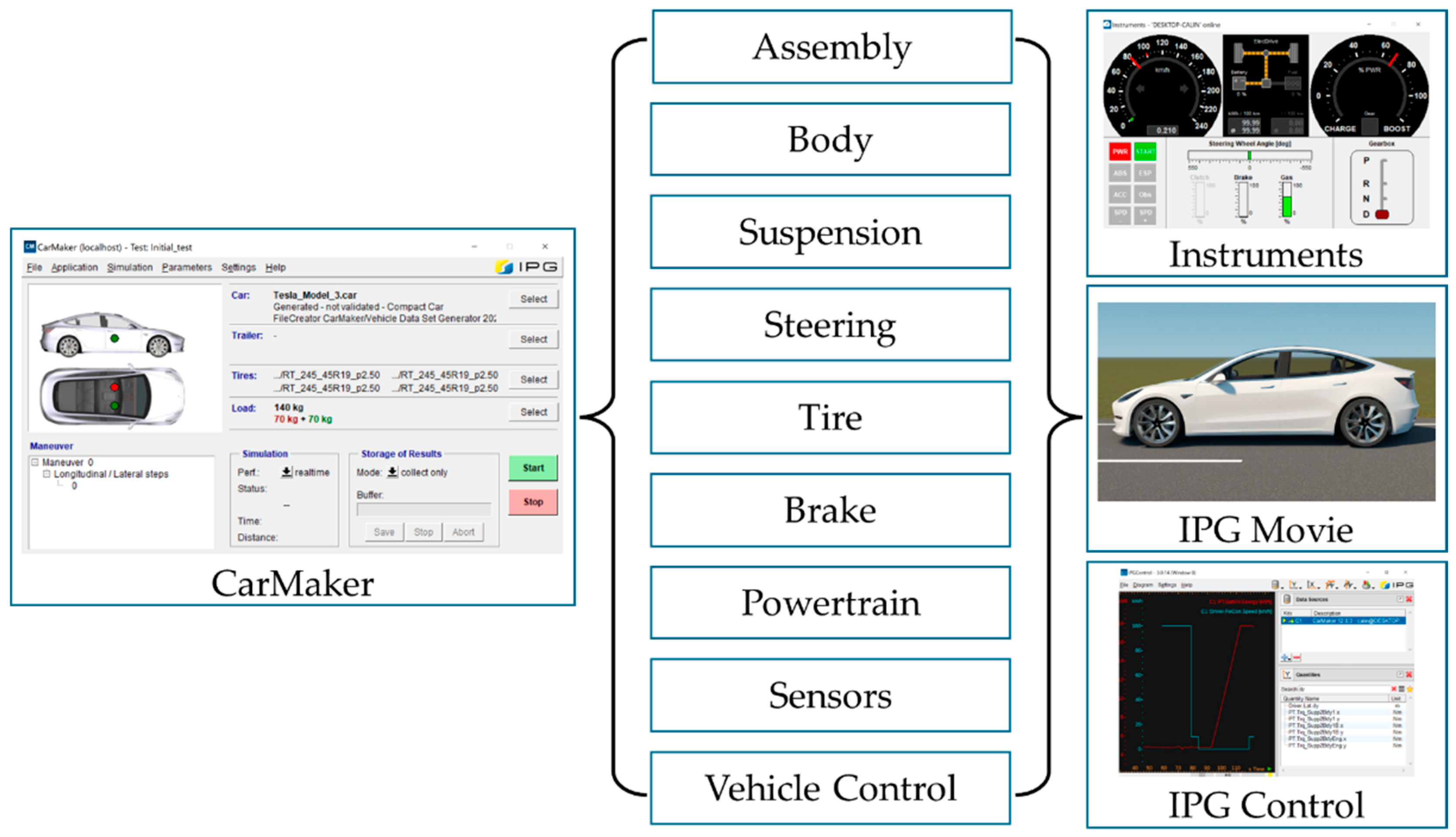
Figure 2.
Virtual vs. real vehicle model for Tesla Model 3.
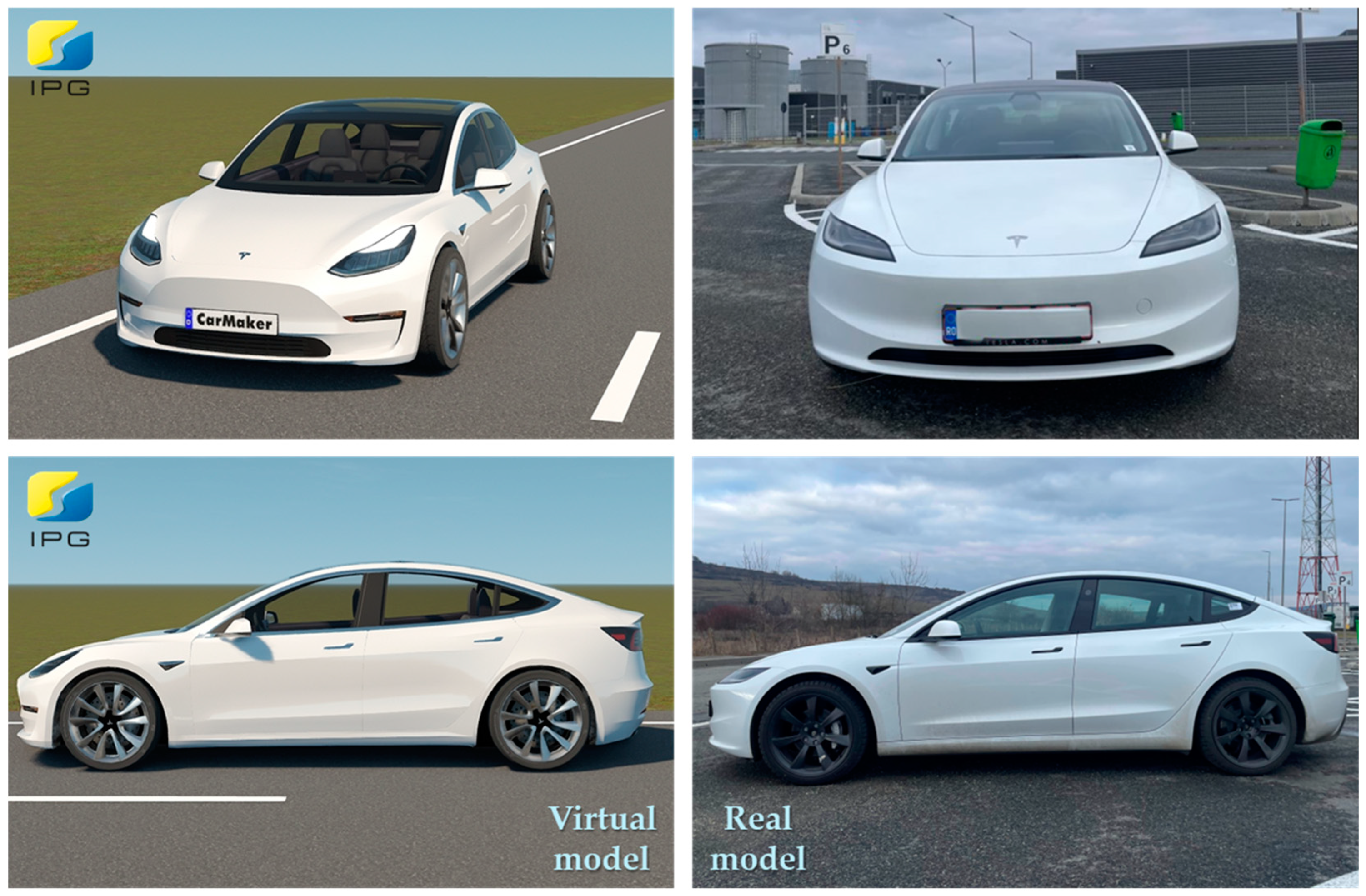
Figure 3.
Torque/Power characteristics for electric motors of Tesla Model 3.
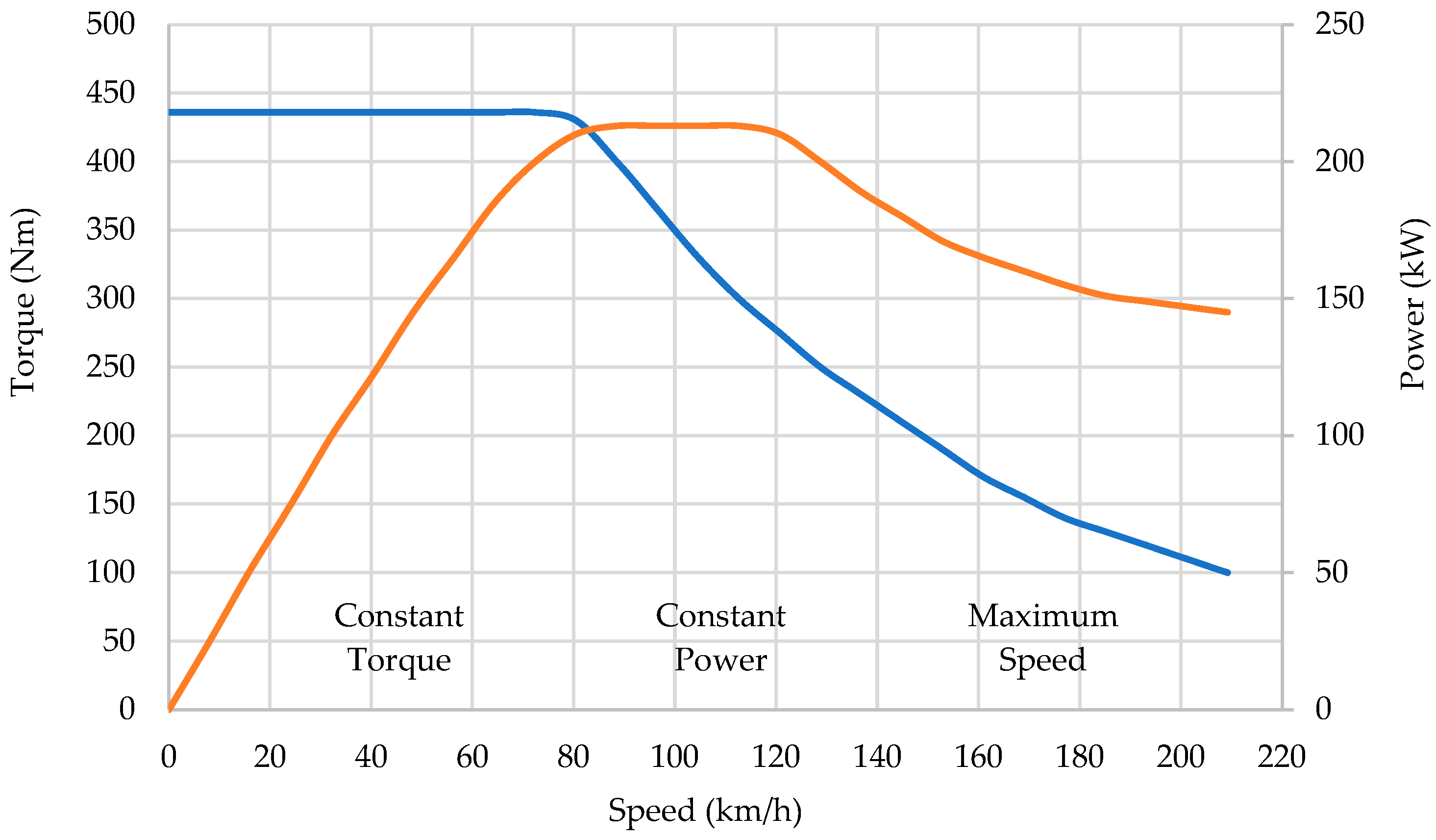
Figure 4.
Power supply model (LV; LV+HV1; LV+HV1+HV2).
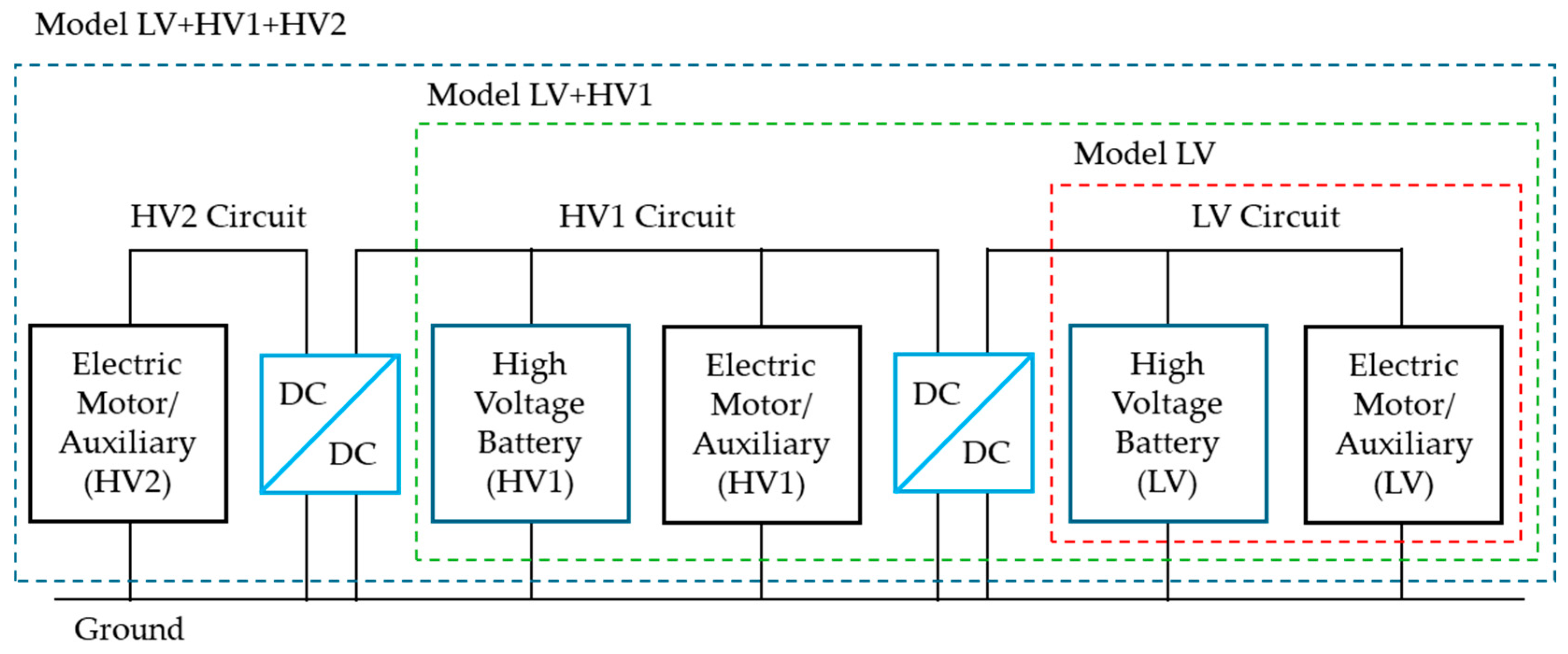
Figure 5.
Structure of PTControl module.
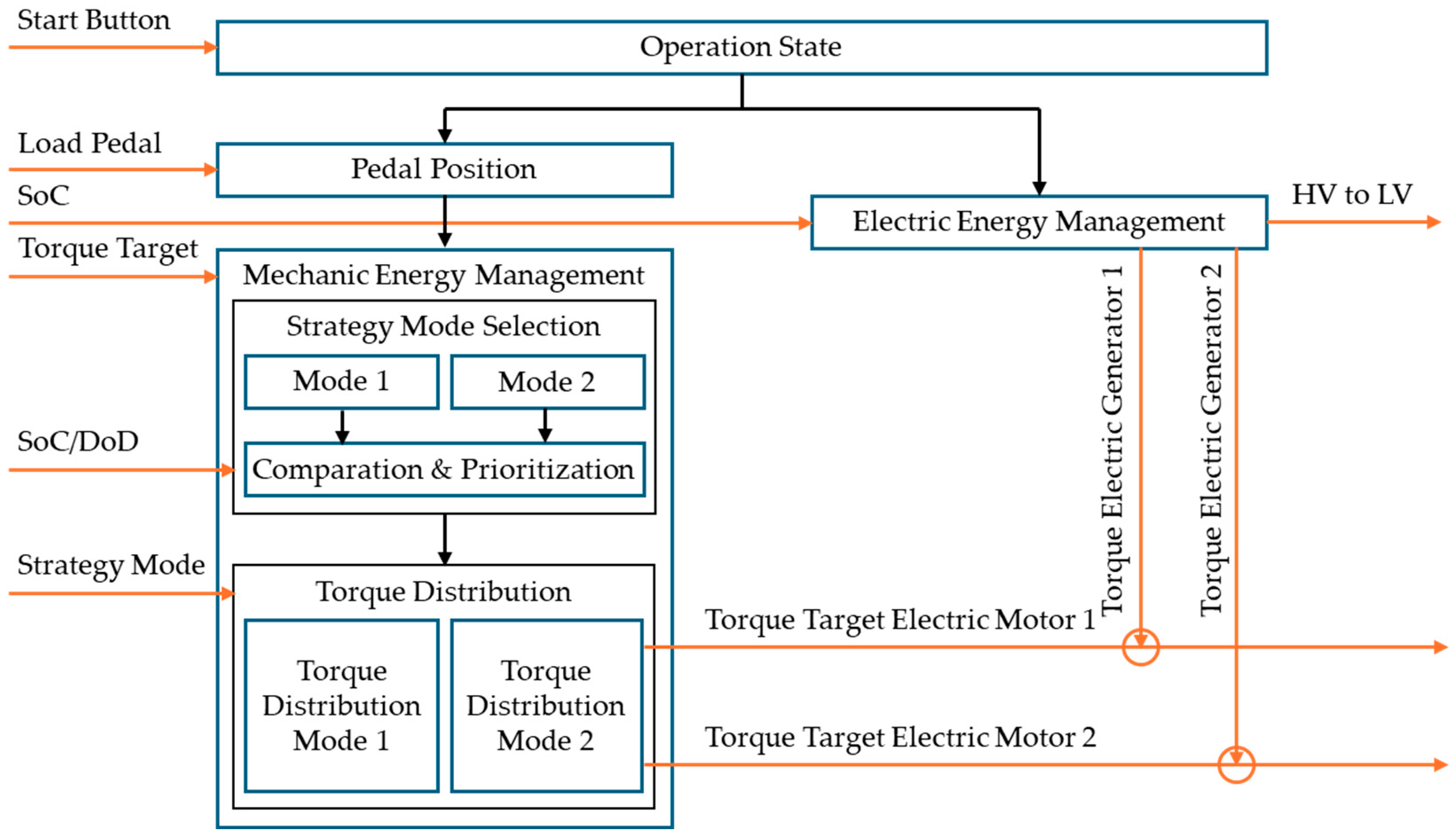
Figure 6.
Virtual road for simulation cycle: (a) WLTC (Worldwide harmonized Light vehicles Test Cycles); (b) FTP-75 (Federal Test Procedure); (c) HWFET (Highway Fuel Economy Test); (d) ARTEMIS (Assessment and Reliability of Transport Emission Models and Inventory Systems) urban; (e) JC08 (Japanese Cycle); (f) NYCC (New York City Cycle).
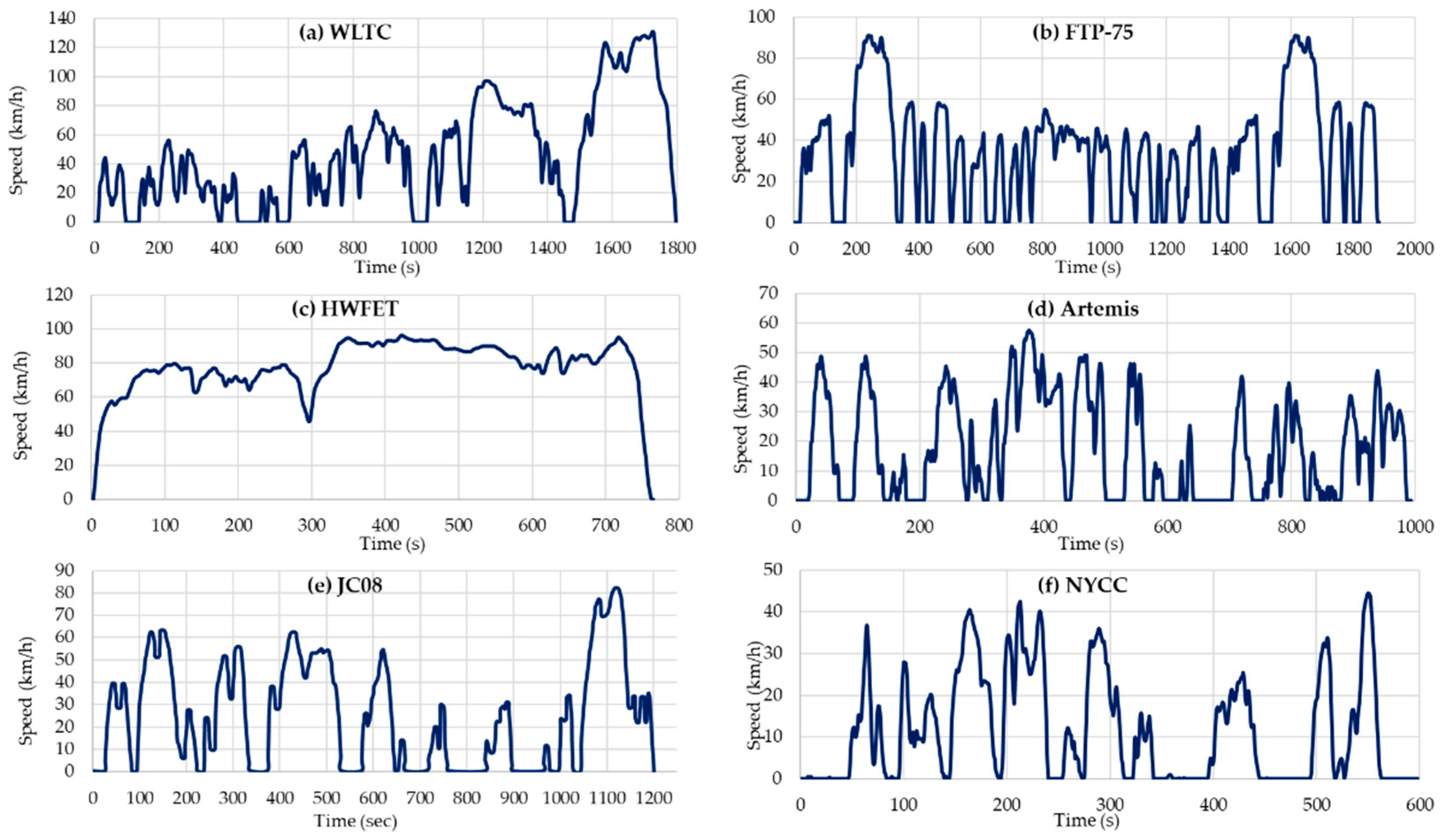
Figure 7.
Virtual road for metropolitan area in IPGRoad: (1) Extra-urban metropolitan area 1; (2) Metropolitan ring; (3) Extra-urban metropolitan area 2; (4) Urban metropolitan area; (5) Urban peripheral area 1; (6) Urban central area; (7) Urban peripheral area 2.
Figure 7.
Virtual road for metropolitan area in IPGRoad: (1) Extra-urban metropolitan area 1; (2) Metropolitan ring; (3) Extra-urban metropolitan area 2; (4) Urban metropolitan area; (5) Urban peripheral area 1; (6) Urban central area; (7) Urban peripheral area 2.
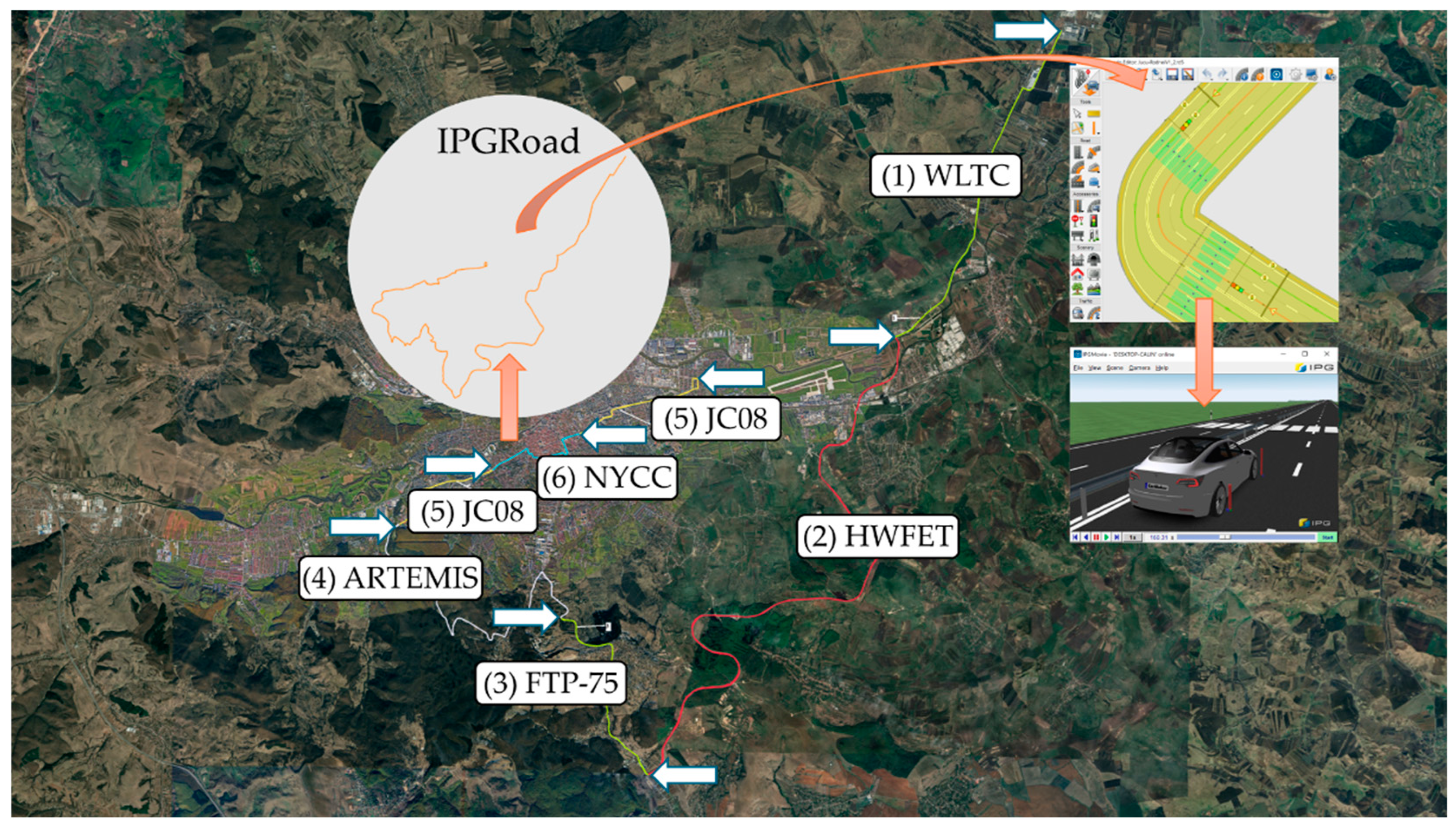
Figure 8.
IPGDriver input and output parameters.
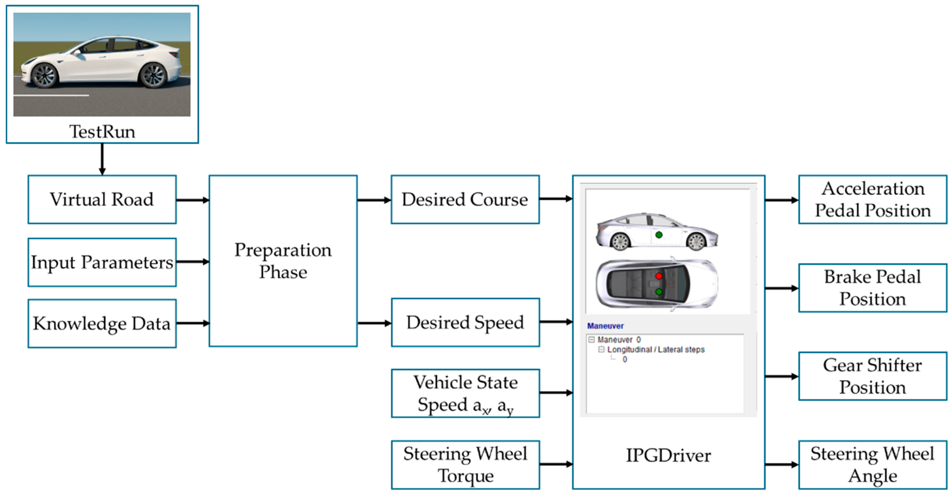
Figure 9.
Radar cross section of the various objects (vehicle, truck, pedestrian).
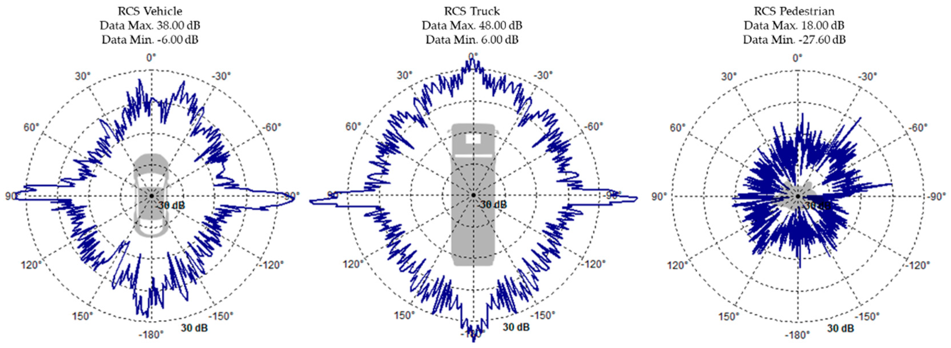
Figure 10.
Driver-in-the-Loop Simulator with Tesla Model 3 Virtual Model in CarMaker.
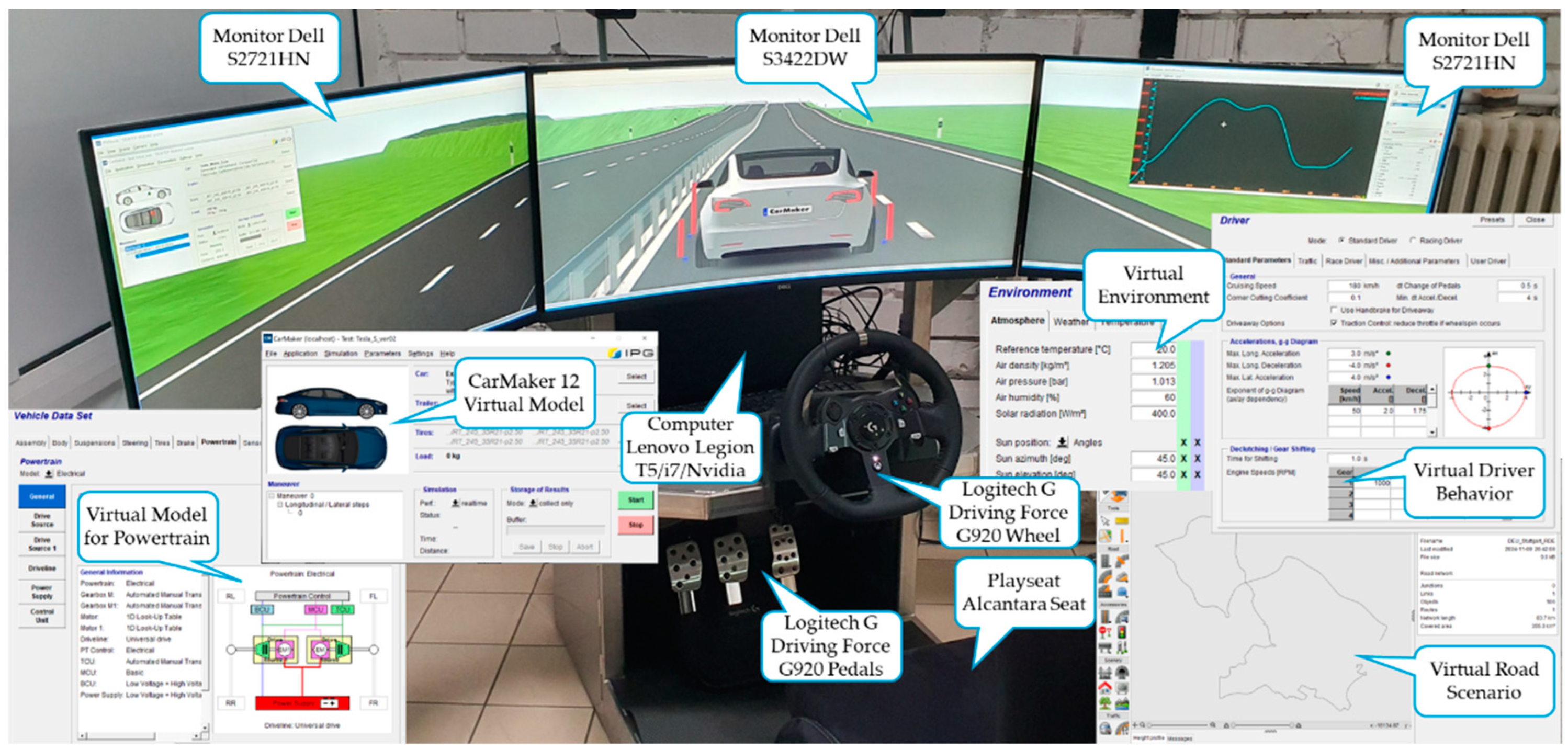
Figure 11.
Energy consumption for the considered driving cycles: (a) WLTC (Worldwide harmonized Light vehicles Test Cycles); (b) HWFET (Highway Fuel Economy Test); (c) FTP-75 (Federal Test Procedure); (d) ARTEMIS Urban; (e) JC08 (Japanese Cycle); (f) NYCC (New York City Cycle).
Figure 11.
Energy consumption for the considered driving cycles: (a) WLTC (Worldwide harmonized Light vehicles Test Cycles); (b) HWFET (Highway Fuel Economy Test); (c) FTP-75 (Federal Test Procedure); (d) ARTEMIS Urban; (e) JC08 (Japanese Cycle); (f) NYCC (New York City Cycle).
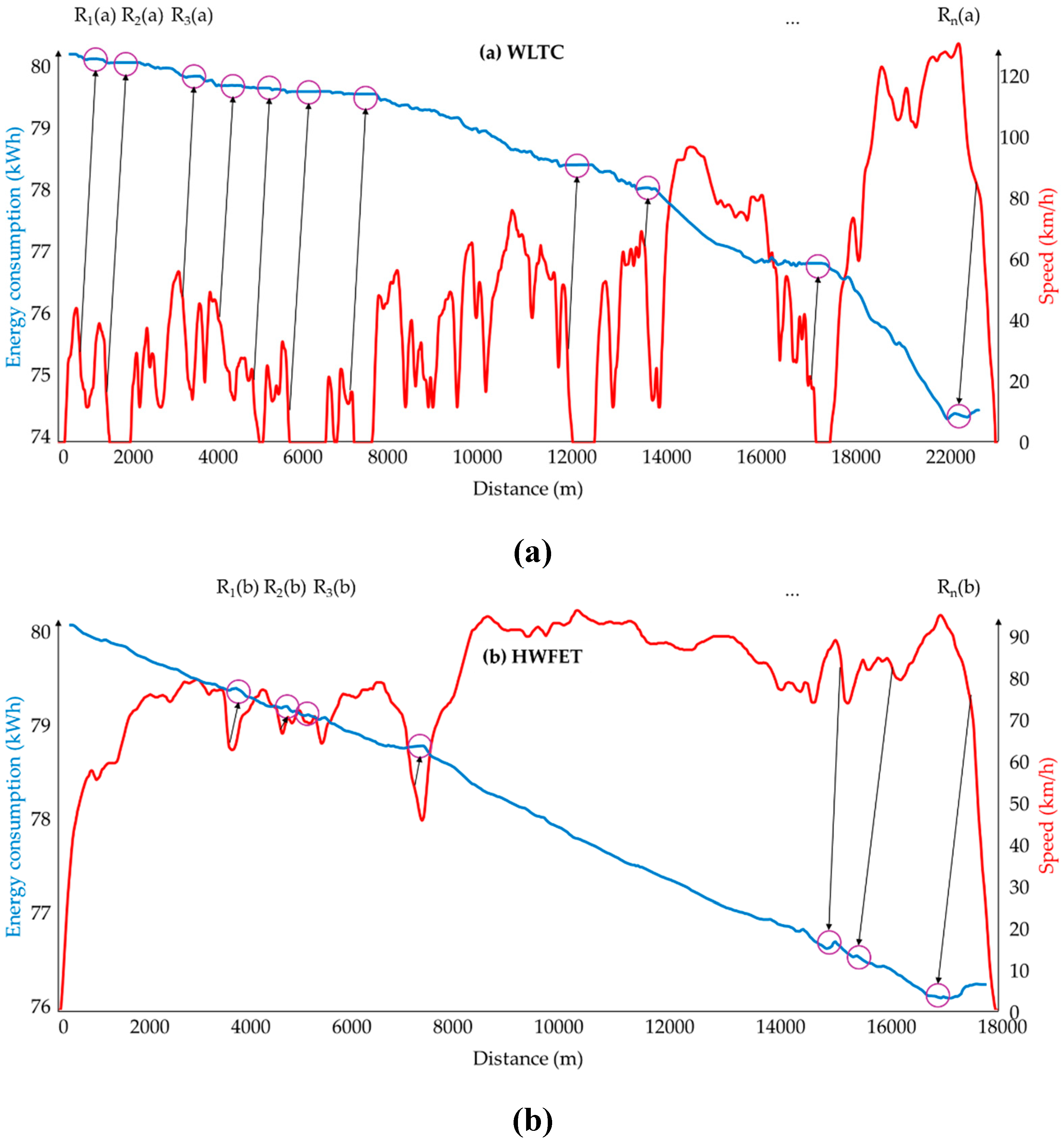
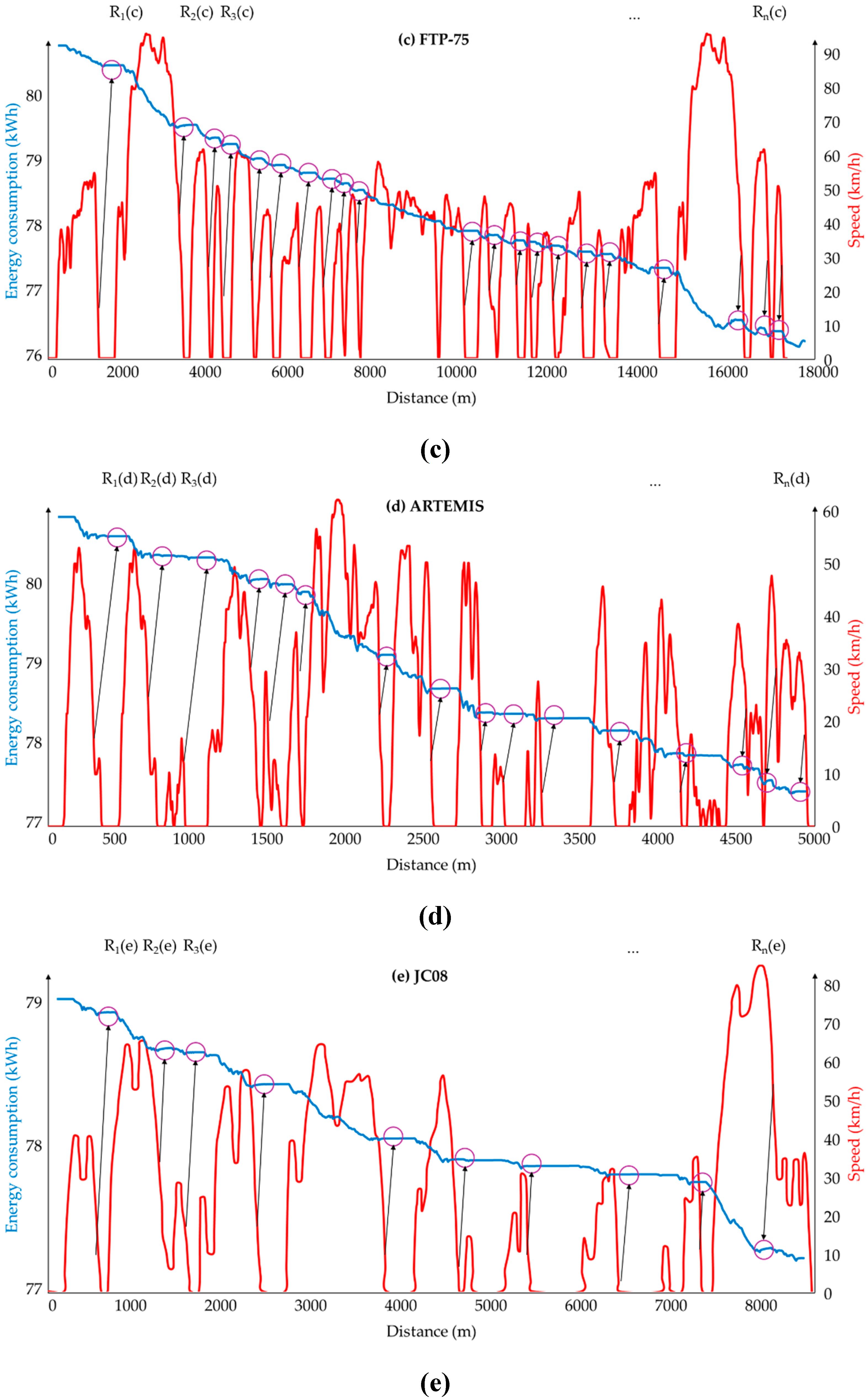
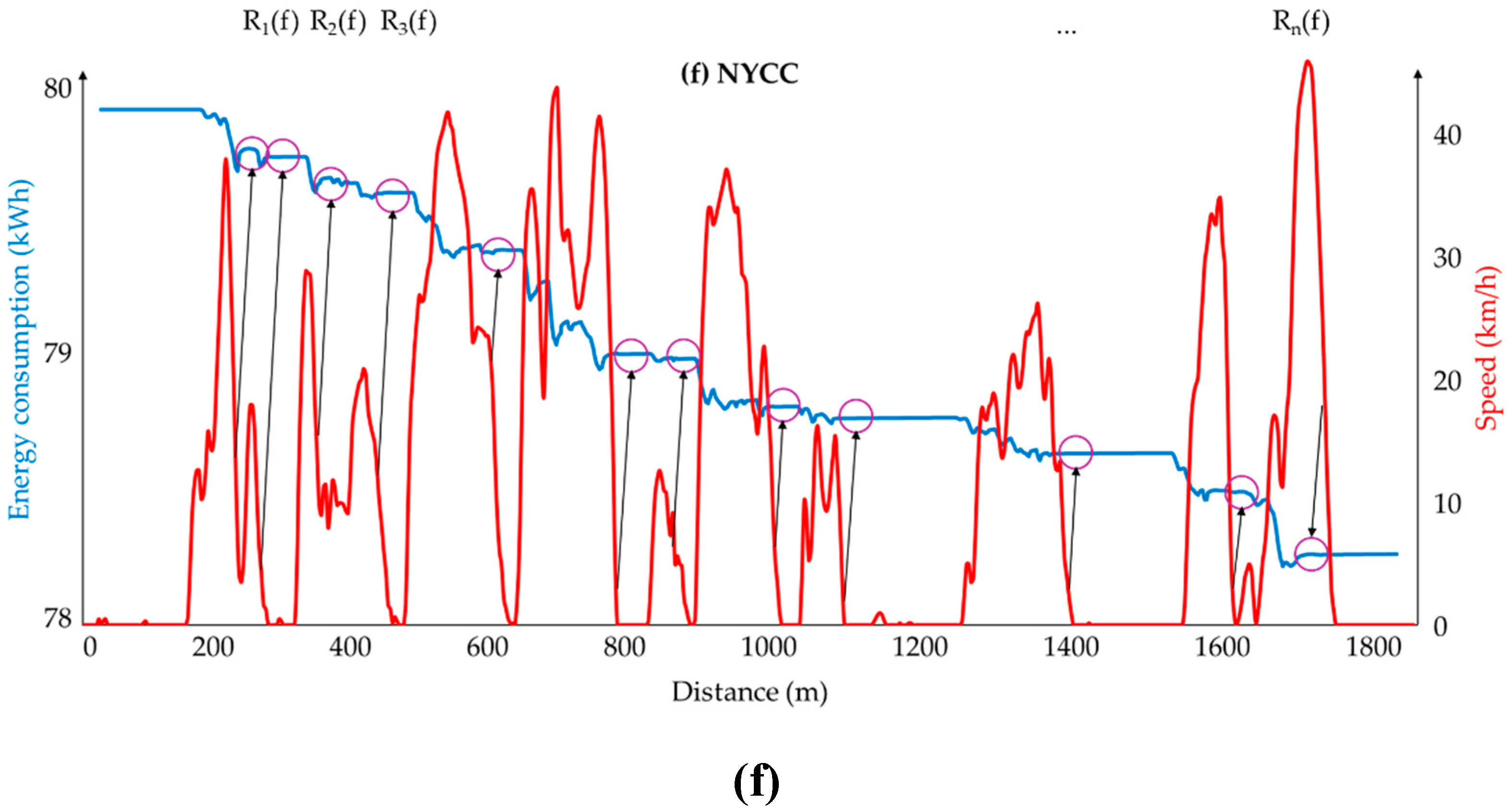
Figure 12.
Evaluation of energy consumption in driving scenarios considered in metropolitan area.
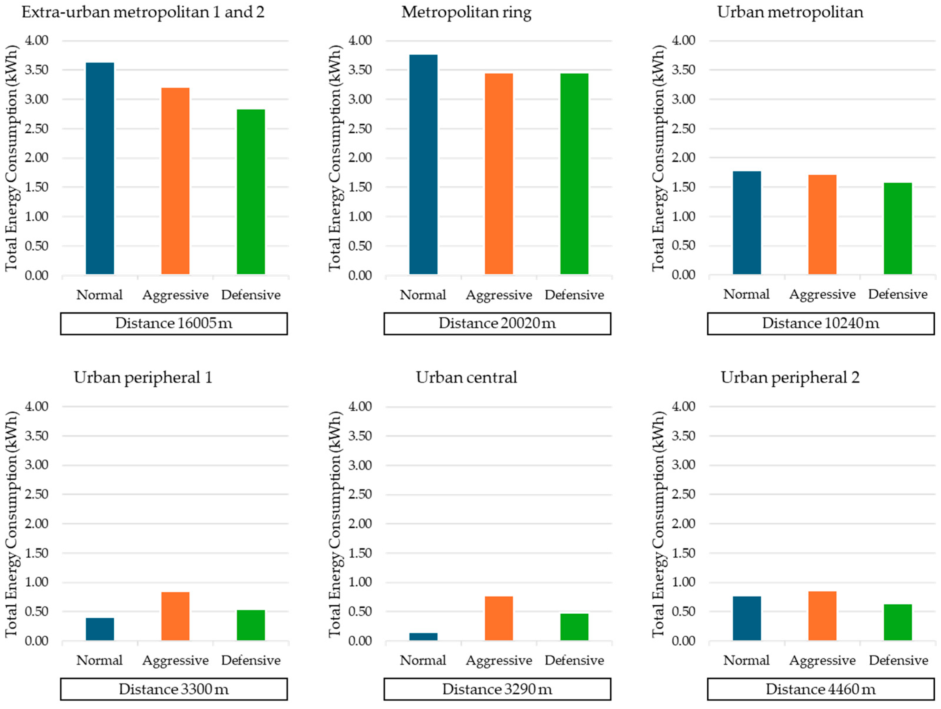

Table 1.
Tesla Model 3 operating performance was used to define the virtual vehicle model in CarMaker.
Table 1.
Tesla Model 3 operating performance was used to define the virtual vehicle model in CarMaker.
| Parameters | Unit | Value |
|---|---|---|
| Maximum motor power (6000-9500 1/min) | kW | 213 |
| Maximum motor torque (0-5800 1/min) | Nm | 436 |
| Battery energy storage | kWh | 78 |
| Battery nominal voltage | VDC | 357 |
| Battery number of cells [26] | - | 4416 |
| Battery pack configuration (serial/parallel) [26] | - | 96s46p |
| Rapid charging (supercharger V3 up to 282 km) | min | 15 |
| Energy consumption | kWh/km | 0.14 |
| Estimate range (EPA-FTP-75 range test [27]) | km/kWh/km | 488/0.16 |
| Estimate range (WLTP range test [28]) | km/kWh/km | 528/0.15 |
| Certified range (0 to 100 km/h) | s | 5.2 |
| Maximum speed | km/h | 201 |
Table 2.
Tesla Model 3 dimensions and weights were used to define the virtual vehicle model in CarMaker.
Table 2.
Tesla Model 3 dimensions and weights were used to define the virtual vehicle model in CarMaker.
| Parameters | Unit | Value |
|---|---|---|
| Overall length | mm | 4720 |
| Overall width (including mirrors) | mm | 2089 |
| Overall height | mm | 1442 |
| Wheelbase | mm | 2875 |
| Overhang front/rear | mm | 868/977 |
| Ground clearance | mm | 138 |
| Track wheels front/rear | mm | 1584/1584 |
| Curb Mass (no occupants and no cargo) | kg | 1823 |
| Technically permissible maximum laden mass | kg | 2255 |
| Maximum payload | kg | 432 |
Table 3.
Driving cycle characteristics as integrated into CarMaker/Scenario Editor/Maneuver.
| Parameters | WLTC | FTP-75 | HWFET | ARTEMIS | JC08 | NYCC |
|---|---|---|---|---|---|---|
| Distance (m) | 23266 | 17769 | 16503 | 4874 | 8159 | 1902 |
| Duration (s) | 1800 | 1877 | 765 | 993 | 1204 | 598 |
| Maximum speed (km/h) | 131.30 | 91.25 | 96.32 | 57.32 | 81.60 | 44.45 |
| Average cycle speed (km/h) | 46.53 | 34.08 | 77.70 | 17.70 | 24.40 | 11.50 |
| Average driving speed (km/h) | 53.21 | 41.57 | 77.76 | 22.29 | 34.24 | 16.63 |
| Driving time (s) | 1574 | 1539 | 759 | 787 | 858 | 412 |
| Maximum acceleration (m/s2) | 1.67 | 1.48 | 1.43 | 2.86 | 1.69 | 2.68 |
| Average acceleration (m/s2) | 0.41 | 0.51 | 0.20 | 0.53 | 0.43 | 0.00 |
| Acceleration time (s) | 789 | 739 | 264 | 357 | 435 | 176 |
| Number of acceleration (-) | 68 | 78 | 26 | 48 | 46 | 22 |
| Acceleration per km (m/s2) | 2.92 | 4.39 | 1.58 | 9.85 | 5.64 | 11.56 |
| Minimum deceleration (m/s2) | -1.50 | -1.48 | -1.48 | -1.48 | -1.22 | -1.50 |
| Average deceleration (m/s2) | -0.45 | -0.58 | -0.22 | -0.57 | -0.46 | -0.48 |
| Deceleration time (s) | 719 | 655 | 210 | 335 | 405 | 175 |
| Standing time (s) | 226 | 338 | 1 | 206 | 346 | 186 |
| Number of stops (-) | 8 | 19 | 1 | 14 | 11 | 7 |
| Maximum stop time (s) | 66 | 38 | 6 | 15 | 76 | 27 |
| Stop per km (-) | 0.34 | 1.07 | 0.06 | 2.87 | 1.35 | 3.68 |
Table 4.
Model GLxC (generic longitudinal control) for vehicle movement.
| Parameters | Unit | Value |
|---|---|---|
| Autonomous emergency braking | ||
| Referenced object sensor | - | Front radar |
| Maximal deceleration | m/s2 | 6.0 |
| Acceleration controller factor P (proportional) | - | 0.001 |
| Acceleration controller factor I (integral) | - | 3.0 |
| Minimal distance | m | 5.0 |
| Time braking after standshill | s | 5.0 |
| Time brake reacts | s | 0.2 |
| Forward collision warming | ||
| Time first warming level | s | 2.0 |
| Time second warming level | s | 1.0 |
Table 5.
Model GLyC (generic lateral control) for vehicle direction.
| Parameters | Unit | Value |
|---|---|---|
| Initial line detection mode | - | Line sensor |
| Line keeping assist system | ||
| Maximal velocity | km/h | 55.0 |
| Maximal assist torque | Nm | 2.0 |
| Time constant PT (powertrain) filter | s | 0.003 |
| Maximal lane width | m | 7.0 |
| Minimal line width | m | 1.8 |
| Curvature controller factor P (proportional) | - | 2.0 |
| Curvature controller factor I (integral) | - | 0.2 |
| Curvature controller factor D (derivative) | - | 0.0 |
| Maximal deviation distance | m | 10.0 |
| Assist torque coefficient | Ns2 | 2.0 |
| Lane departure warning | ||
| Maximal velocity | km/h | 55.0 |
| Distance departure warning | m | 0.2 |
Table 6.
Characteristic parameters for standard driver driving mode.
| Standard driver driving mode |
Longitudinal acceleration (m/s2) |
Longitudinal deceleration (m/s2) |
Lateral acceleration (m/s2) |
|---|---|---|---|
| Driver Presets Standard normal | 3.00 | -4.00 | 4.00 |
| Driver Presets Standard defensive | 2.00 | -2.00 | 3.00 |
| Driver Presets Standard aggressive | 4.00 | -6.00 | 5.00 |
Table 7.
Characteristic parameters for extended driver driving mode.
| Extended driver driving mode | Dynamics | Energy efficiency | Nervousness |
|---|---|---|---|
| Energy efficient driver | 0.20 | 0.10 | 0.00 |
| Stressed driver | 0.70 | 0.00 | 0.50 |
Table 8.
Experimental results in metropolitan area (real vehicle Testa Model 3).
| Area | Length (m) | Average speed (km/h) | Energy consumption (kWh/km) | Recovered energy (kWh/km) | Total energy (kWh/km) |
|---|---|---|---|---|---|
| Extra-urban metropolitan 1 | 10030 | 54.99 | 0.177 | 0.031 | 0.146 |
| Metropolitan ring | 20020 | 81.30 | 0.269 | 0.023 | 0.269 |
| Extra-urban metropolitan 2 | 5970 | 54.40 | 0.187 | 0.009 | 0.178 |
| Urban metropolitan | 10240 | 42.00 | 0.172 | 0.029 | 0.143 |
| Urban peripheral 1 | 3330 | 17.48 | 0.130 | 0.011 | 0.119 |
| Urban central | 3290 | 15.70 | 0.173 | 0.010 | 0.163 |
| Urban peripheral 2 | 4460 | 21.00 | 0.179 | 0.016 | 0.163 |
Table 9.
Simulation results in metropolitan area (virtual model Tesla Model 3 on Driver-in-the-Loop simulator).
Table 9.
Simulation results in metropolitan area (virtual model Tesla Model 3 on Driver-in-the-Loop simulator).
| Area | Length (m) | Average speed (km/h) | Energy consumption (kWh/km) | Recovered energy (kWh/km) | Total Energy (kWh/km) |
|---|---|---|---|---|---|
| Extra-urban metropolitan 1 | 10035 | 54.99 | 0.170 | 0.020 | 0.150 |
| Metropolitan ring | 20020 | 81.30 | 0.220 | 0.025 | 0.195 |
| Extra-urban metropolitan 2 | 5970 | 54.40 | 0.180 | 0.010 | 0.170 |
| Urban metropolitan | 10240 | 42.00 | 0.165 | 0.030 | 0.135 |
| Urban peripheral 1 | 3330 | 17.48 | 0.125 | 0.015 | 0.110 |
| Urban central | 3290 | 15.70 | 0.160 | 0.010 | 0.150 |
| Urban peripheral 2 | 4460 | 21.00 | 0.170 | 0.020 | 0.150 |
Table 10.
Simulation results in Metropolitan area (virtual model Tesla Model 3 on driving cycles).
| Driving cycle | Cycle length (m) | Normal driving behavior | Aggressive driving behavior | Defensive driving behavior | |||||||
|---|---|---|---|---|---|---|---|---|---|---|---|
| Average speed (km/h) | Energy consumption (kWh/km) |
Energy recovered (kWh/km) |
Average speed (km/h) | Energy consumption (kWh/km) |
Energy recovered (kWh/km) |
Average speed (km/h) | Energy consumption (kWh/km) |
Energy recovered (kWh/km) |
|||
| (1) WLTC | 23266 | 46.13 | 0.188 | 0.040 | 46.07 | 0.201 | 0.000 | 40.32 | 0.173 | 0.005 | |
| (2) HWFET | 16503 | 77.67 | 0.166 | 0.023 | 77.54 | 0.173 | 0.000 | 72.38 | 0.155 | 0.018 | |
| (3) FTP-75 | 17769 | 34.11 | 0.162 | 0.014 | 34.07 | 0.169 | 0.000 | 30.99 | 0.150 | 0.006 | |
| (4) ARTEMIS | 51687 | 17.63 | 0.183 | 0.003 | 17.60 | 0.256 | 0.000 | 15.66 | 0.163 | 0.002 | |
| (5) JC08 | 8159 | 24.42 | 0.174 | 0.003 | 24.39 | 0.194 | 0.000 | 21.93 | 0.145 | 0.002 | |
| (6) NYCC | 1902 | 11.38 | 0.216 | 0.002 | 11.34 | 0.235 | 0.000 | 9.57 | 0.198 | 0.002 | |
Disclaimer/Publisher’s Note: The statements, opinions and data contained in all publications are solely those of the individual author(s) and contributor(s) and not of MDPI and/or the editor(s). MDPI and/or the editor(s) disclaim responsibility for any injury to people or property resulting from any ideas, methods, instructions or products referred to in the content. |
© 2025 by the authors. Licensee MDPI, Basel, Switzerland. This article is an open access article distributed under the terms and conditions of the Creative Commons Attribution (CC BY) license (http://creativecommons.org/licenses/by/4.0/).
Copyright: This open access article is published under a Creative Commons CC BY 4.0 license, which permit the free download, distribution, and reuse, provided that the author and preprint are cited in any reuse.


