Submitted:
03 May 2025
Posted:
06 May 2025
Read the latest preprint version here
Abstract
This paper presents a methodology for systematically scaling vehicle powertrain and other models and an approach for using model parameters and scaling variables to perform controller design. The parameter scaling method allows for high degrees of scaling while maintaining the target performance metrics, such as vehicle speed tracking, with minimal changes to model code by the researcher. A comparison of proportional-integral, Youla parameterization, H∞, and hybrid Youla-H∞ controllers is provided along with the respective methods for maintaining controller performance metrics across degrees of model scaling factors. The application of the scaling and various control design methods to an existing model of a hydrogen fuel cell and a battery electric vehicle powertrain allows for the development of a representative scale model to be compared with experimental data generated by an actual scale vehicle. The comparison between scaled simulation and experimental data will eventually be used to inform the expected performance of the full-size electric vehicle based on full-size simulation results.
Keywords:
Powertrain Scaling
; Controller Design
; H∞ Control
; Youla Parameterization
; Scale Model Validation
1. Introduction
Previous work on the development of a model for hydrogen proton-exchange membrane fuel cells (PEMFC) [1] and on electric vehicle (EV) powertrains [1] resulted in a detailed simulation to be used for evaluating energy management strategies between the PEMFC and the battery during the execution of various drive cycles.
This prior work is important in supporting the exploration of alternative energy systems for transportation. Higher efficiency energy management strategies contribute towards the reduced cost and environmental impact of EVs. To further support this prior and ongoing work, a faster way to test these energy management strategies is necessary. The development of small-scale PEMFC plus battery test vehicles allows for rapid evaluation of efficiency at low cost. The validation of the small-scale simulation models against the scaled test vehicles allows for the estimation of performance for full-scale models, informing potential future developments for full-scale vehicles.
1.1. Powertrain Model
The vehicle model is comprised of vehicle, motor, fuel cell, and battery dynamics. Figure 1 shows the model architecture.
The fuel cell model is described in [1]. The design of the fuel cell controller is outside the scope of this paper. Relevant to the scaling methodology, the PEMFC is comprised of a stack of individual fuel cells in series with identical dynamics. The number of cells in the fuel cell stack is the only variable in the fuel cell block that will change as the system scales. The battery uses the standard Simulink battery block, and the voltage outputs of the fuel cell and battery are reconciled by a DC-DC converter before the final voltage is supplied to the motor controller.
The energy management system block represents the strategy for choosing whether to power the vehicle from the fuel cell or the battery, given the current power required by the vehicle, the battery state-of-charge (SOC), and the capabilities of the fuel cell. The design of the energy management system is the primary area of active research. Its development, while outside the scope of this paper, is what this paper aims to support.
The driver control block uses the drive cycle reference speed and the vehicle’s actual speed to calculate target torques via proportional-integral (PI) with feedforward, Youla, or control.
For the results in this paper, the motor dynamics are assumed to be significantly faster than vehicle dynamics, and so the target torque is immediately applied to the vehicle dynamics if possible. The motor block may saturate the torque output, with the maximum torque available decreasing as the motor rotational speed increases. This is a nonlinear effect that the controllers compensate for by being robust. A 3-phase permanent-magnet synchronous motor (PMSM) model [1] of motor dynamics, developed via a bond graph approach in [1], allows for transient voltage estimates that are more accurate to the actual EV. The PMSM model is omitted in this paper for simplicity, but may be added in the future. The PMSM model is mentioned in order to discuss the difficulties it presents in scaling its dynamics.
The vehicle dynamics accounts for vehicle mass, viscous friction, motor inertia, gearing, air resistance, and tire slip. Future versions of this model will also incorporate series regenerative braking to maximize energy efficiency, using friction braking only when absolutely necessary. In this paper, all braking is done with regenerative braking irrespective of battery SOC limits. Future work will incorporate these limits.
1.2. Dimensional Analysis
The Buckingham Pi (BP) theorem in dimensional analysis [2] is a common approach to develop scale system models. The BP method computes dimensionless parameters from a given set of input variables to the equation being analyzed based on the physical units of those input variables. If the dimensionless parameters are held constant when changing the parameters of the model, then the model is considered to have various potential degrees of similitude and thus to be representative of full-scale behavior. This method requires solving systems of linear equations and can be unwieldy when repeatedly applied. It is best suited for equations involving a large number of parameters or when an explicit relationship may not be known.
The vehicle powertrain model in question consists of many simple equations with few relevant parameters rather than fewer equations with more parameters. Rather than repeatedly applying the BP theorem, the model can be systematically scaled with an easy inspection of the governing equations with the method presented in this paper, which could be considered a simplified version of the BP theorem.
1.3. Control Methods
A proportional-integral (PI) controller with reference feedforward is examined, representing the baseline controller performance of traditional methods. The PI gains were initially determined via experimentation and then tuned by considering the closed-loop transfer functions in order to set the controller bandwidth to be the same on each controller described in this paper. In order to keep system performance constant throughout scaling magnitudes, the PI gains have a specific scaling factor to keep the dynamics constant.
Youla parameterization [3] is a technique in neoclassical control theory that provides robust controller performance, where robustness is defined as the insensitivity of system performance to changes in system parameters, such as vehicle mass, friction, etc. The Youla controller can be developed analytically, given a linear model of the plant and the desired closed-loop behavior, which in this paper is a second-order response with a damping ratio of 1.0. With an appropriately scaled model, controller tuning will be independent of the scale of the system and will not need to be performed by the user across scaling magnitudes. Due to the robust nature of Youla parameterization, performance can be maintained despite system nonlinearities that are not captured by the scaling method. Since the controller is calculated by the system parameters directly, it does not require any scaling factors specific to the controller.
control [3] is another neoclassical control technique that provides optimally robust performance, given the designer’s closed-loop response priorities. These priorities are represented as weighting functions on the closed-loop transfer functions, which are provided to an optimization algorithm to produce the controller transfer function that maximizes robustness given the weighting functions. Since the closed-loop sensitivity and complementary sensitivity transfer functions S and T, respectively, are ratios in the frequency domain, they do not change as the system parameters are scaled. However, the Youla transfer function Y, which represents the actuator effort, does scale with the actuator size and so must have a scaling factor applied in order for the optimization algorithm to produce the same dynamics across scaling magnitudes.
Finally, a hybrid Youla and approach is performed, which uses the poles and zeros of the Y transfer function produced by the algorithm as the input to the Youla parameterization method. This allows for performance improvements without sacrificing robustness by making small adjustments to ensure that exact reference tracking is possible. This also allows for the controller to be calculated by the plant parameters without requiring a specific controller scaling factor.
All controllers are selected so that the closed-loop system bandwidth is approximately 24 rad/sec. Among other aspects, the bandwidth corresponds to the reaction speed of the controller, and keeping this metric constant makes the comparisons of tracking error, robustness, and noise attenuation between controllers meaningful when applied to a drive cycle where the reference velocity is rapidly changing. The value of 24rad/sec was found to be a good balance of tracking performance and noise attenuation, given the rate at which common drive cycles change their reference target speed.
2. Scaling Method
The scaling method utilized consists of the following steps:
- List equations that define the behavior of the model.
- Begin determining what variables and parameters will be scaled.
- Determine the scaling relationship for each equation.
- Develop the complete list of scaled variables while performing the previous step.
- Check for relationships that over-constrain the scaling system and decide which scaling factors are to be considered the "independent" factors input to the system.
Scaling parameters will be denoted , where x is the parameter being scaled and are defined as:
2.1. Simple Example
A simple model to examine the scaling method is as follows. Suppose a mass-spring-damper system as shown in Figure 2.
Step 1: Write the governing equation(s):
Step 2: Determining the variables to be scaled. Here, it would be the mass, length, spring constant, and damping constant. Note that the acceleration, position, and velocity scale with the same length scaling, since they are time derivatives or integrals of each other.
Step 3: Determine the scaling relationship for each equation. To do this, first replace each original variable with its new variable, given by . Since they are time-derivatives of each other, the acceleration, velocity, and position can all be modified by a single length scaling parameter . This assumes that the timescale is not being changed, otherwise the velocity and acceleration would need a time-scaling factors applied.
Factoring out the length scaling results in:
By inspection, it is obvious that for the dynamics to remain unchanged, . Satisfying this relationship keeps the characteristics of the dynamics the same, only scaling up or down the numerical values of the system variables as if only changing the units of the system.
The more general approach is to determine the scaling relationship required to be able to factor out all of the scalings from the equation and be left only with the variables present in the original equation. The left side can only be canceled out if .
Step 4: Develop a complete list of scaled variables. In this case, it is , as well as . This step is complete because there was only one equation. The purpose of step 4 is to allow for the list of scalings to grow as the equations are analyzed. That list of scalings can be condensed such as shown above, with representing the scaling for the acceleration, velocity, and position all at once – or it can be fully verbose and maintain separate nomenclature such as with the subsequent constraint that .
Step 5: Since there was only one governing equation and that equation is easily solvable, there cannot be over-constraints. An example of a potential conflict would be the introduction of air resistance:
Which becomes:
This introduces a complex requirement that , with the drag coefficient itself being a nonlinear function of the Reynolds number. It is unlikely that the drag coefficient can be easily adjusted to meet the above requirement, and the effort that goes into satisfying that requirement relative to its importance to the model determines whether air resistance or other similar aspects should be omitted from the scaling system (not from the simulation model). This case could potentially be solvable, but other cases will be fully unsolvable.
If air drag is omitted from the scaling system, then is the only remaining equation defining system behavior. The resulting scaling relationship indicates that there are two degrees of freedom (DOFs). One independent scaling must be either the length or input force scaling for set one DOF. The second DOF is described by , where any one of these three can be chosen to be the second input variable, full defining the scaling system.
3. System Modeling
With the above example complete, the analysis of the actual EV powertrain model is described in this section.
The goal of scaling this model is to preserve the velocity-tracking performance of the vehicle during drive cycles, such as the FTP75 drive cycle, and subsequently estimate the hydrogen consumption performance for different battery management strategies.
3.1. Step 1: Governing Equations
The governing equations are grouped into those relating to the vehicle, controller, and electrical dynamics.
3.1.1. Vehicle Dynamics
Equation 1 represents the mechanical power imparted to the vehicle system. is the force at the wheel and v is the speed of the car.
Equation 2 gives the force at the wheel, where m is the total mass of the vehicle, a is the vehicle’s acceleration, and is the drag force due to air resistance.
Equation 3 provides the drag force, where is air density, v is the vehicle speed, is the drag coefficient, and A is the vehicle cross-sectional area.
Equation 4 shows the relationship between the torque at the wheel and the force at the wheel, with r being the wheel radius.
Equation 5 is the torque at the motor, where is the gear ratio, is an efficiency factor in converting motor torque to wheel torque, J is the motor moment of inertia, is the motor angular acceleration, b is the motor viscous friction, and is the motor angular velocity.
Equation 6 defines the relationship between the motor and wheel rotational velocity through the gear ratio.
Equation 7 gives the braking torque as a function of the braking friction coefficient , the disc brake diameter , the number of brake pads , and the braking pressure .
3.1.2. Controller Dynamics
Equation 8 describes the output of the baseline PI plus feedforward controller that the Youla controller will be compared against. , , and represent the proportional, integral, and feedforward gains, respectively. is the maximum motor torque, e is the velocity tracking error, and is the current target velocity.
Equation 9 describes the output of controller transfer function. This is required to determine the scaling factor for the actuator weighting function given to the optimization algorithm.
3.1.3. Electrical Dynamics
Equation 10 [1] provides the fuel cell stack voltage in terms of the number of fuel cells N, the fuel cell internal voltage E (determined by reactant partial pressures and electrochemistry), the cell layer capacitive voltage , and the ohmic losses . Within the scope of this paper, the internal, capacitive, and ohmic loss voltages will be considered unchanged regardless of scaling, with the fuel cell output voltage scaling only with the number of individual fuel cells.
The battery has an empirical relationship between its output voltage and its state of charge (SOC). Since the SOC is dimensionless, the battery’s output voltage will simply scale with the overall voltage scaling, discussed later. The battery’s capacity will scale with the energy scaling of the system.
3.2. Step 2: Determine the Scaling Variables
By inspecting equations 1 through 10, we can develop the list of scaling variables. To simplify the analysis, the following assumptions are made:
- The vehicle velocity, acceleration, reference velocity, and tracking error all have the same length scaling factor .
- The vehicle size parameters, such as the wheel radius, share the length scaling factor used for velocity.
- The motor angular velocity and angular acceleration share the same rotational scaling factor .
For example, a vehicle sized down 1:10 will use a drive cycle scaled down 1:10. The initial list of scaling variables can be chosen as follows:
- - vehicle and drive cycle length
- - energy/power of vehicle system
- - force at the wheel
- - vehicle mass
- - drag force
- - torque at the wheel
- - torque at the motor
- - gear ratio
- - motor to wheel efficiency
- - motor moment of inertia
- - motor angular velocity
- - motor friction
- - wheel angular velocity
- - braking torque
- - brake disc pressure
- - PI controller gains
- - weighting
- - system voltage
- - fuel cell stack size
- - battery voltage
- - battery capacity
This list was obtained by following equations 1 through 10 and writing the scaling factor for each new variable observed. A subset of these variables are shown in Figure 3 overlaid on the original model architecture diagram.
Note that some scaling parameters are not present, such as force at the wheel, as those parameters are convenient for mathematically defining the scaling system rather than being directly applied to a system parameter. The scaling variables shown in Figure 3 are applied to parameters in their respective blocks. By applying this scaling system, the output signals of each block are, by consequence of how the scaling parameters are defined, scaled to the appropriate degree. This is an important distinction. Scaling parameters are not applied to output signals; they are applied to parameters such that the output signals are scaled correctly.
3.3. Step 3: Develop Scaling Relationships
3.3.1. Vehicle Scaling
Starting with equation 1, the mechanical power imparted to the system, we can determine the scaling relationship by first rewriting equation 1 replacing each original variable with their respective new variable, given by , shown in equation 11.
Equation 11 represents equation 1 for the "new" version of each variable, with those new variables replaced with . Since , dividing the left and right sides of equation 11 by the left and right sides of equation 1 results in equation 12 below, which is the constitutive scaling relationship for equation 1.
The energy scaling of the system (for example, scaling from 40 kW peak power down to 4 W) has to be equal to the scaling of the force at the wheel times the overall length scaling.
For subsequent equations in this section, an abridged version of the process followed above is used. Only the final scaling relationship is described, determined via analysis and inspection.
The scaling relationship for equation 2, the calculation of the force at the wheel, is given by equation 13.
The scaling relationship for equation 3, the drag force, is given by equation 14. This assumes the air density and drag coefficient remain unchanged and that the velocity and frontal area scalings share the same core length scaling.
Note that this presents a constraint to the relationship in equation 13. This will be discussed in more detail in Step 5 of the process.
The scaling relationship for equation 4, the calculation of the torque at the wheel, is given by equation 15.
Using equation 13, equation 15 can equivalently be written as . This type of alternate form can be more intuitive to understand, but it is recommended to use the form shown in equation 15 when implementing in code.
The scaling relationship for equation 5, the calculation of the torque at the motor, is given by equation 16.
The scaling relationship for equation 6, the motor to wheel angular velocity, is given by equation 17.
The scaling relationship for equation 7, the friction braking torque, is given by equation 18. This assumes that the coefficient of friction, the number of brake pads, stays constant, and that the size of the disc brake scales with the overall length scaling. To relate the braking torque to the rest of the vehicle, the braking torque must additionally scale with the torque at the wheel.
3.3.2. Controller Scaling
The scaling relationship for equation 8, the PI controller gains, is given by equation 19. Note that in equation 8, the left and right sides of the equation are both multiplied by an motor torque, so the scalings for the terms inside the parentheses are equal to a scaling of 1 due to the motor torque scaling factors canceling on both sides. Also note that the error, its time integral, and the reference velocity all share the same overall length scaling.
The Youla controller does not require a specific scaling factor since its controller is determined by the plant model parameters directly.
The controller is not directly scaled by any factor. Instead, the weighting function that penalizes actuator effort must be scaled to account for the change in the actuator effort relative to input commands as the vehicle parameters are scaled so that the optimization produces the same controller poles and zeros.
3.3.3. Electrical Scaling
3.4. Step 4: Complete List
Auxiliary scalings can be determined in this step if necessary. Because this scaling system was completed prior to the writing of this paper, it is not necessary in this case.
3.5. Step 5: Resolve Constraints and Choose Independent Scalings
Similar to the Simple Example, the drag force equation introduces a constraint to the system, even with its simplifications. Equation 14 shows . Combined with equation 13, this simplifies to . This is solvable, but in the context of this simulation model, it is desirable to control the mass (or energy) and the overall length independently, so the scaling relationship defined by equation 14 will be omitted from the scaling system. Thus, the relative effect of air drag will not exactly scale with the rest of the system. In our case, this is an acceptable approximation, since the modeled air drag will still be scaled down with the frontal area and velocity, and so the change in dynamics is small for reasonable scaling magnitudes.
By analyzing equations 12 through 18, the vehicle scalings, it can be observed that there are four degrees of freedom. The controller scalings are entirely dependent on the vehicle scaling factors and so do not introduce any additional DOFs. The electrical scalings introduce only one extra degree of freedom, being the system voltage. Therefore, the selected independent scaling factors are:
- - vehicle and drive cycle length
- - energy/power of vehicle system
- - gear ratio
- - motor to wheel efficiency
- - voltage
The efficiency scaling only affects the motor-wheel efficiency relationship. The length, energy, and gear ratio scalings define every other vehicle and controller scaling not in the above list, such as the mass scaling. To implement in code, equations 12 through 23 are simply listed prior to running the simulation model, ordered in such a way that the independent scaling factors are defined first and all others are defined in whatever order is most convenient. For example, equation 12 can be rewritten as , and subsequently equation 13 as , or .
Note that the mass could have been selected as the independent variable instead of energy. In the context of this paper, energy is chosen so that the hydrogen consumption can be conveniently selected, which is more important for this model than directly defining the mass. However, the two scenarios are mathematically equivalent.
3.6. Nonlinearities and Simulation Difficulties
This scaling system works very well across a wide range of scaling magnitudes. However, there are some nonlinearities that do not perfectly scale system dynamics. The air resistance mentioned before is one aspect, as well as the voltage, reactant flow, and partial pressure dynamics of individual fuel cells. The fuel cell controller is a robust controller and so is able to compensate for the changes in relative dynamics as the system is scaled. The battery voltage-capacity relationship is also not linear, so the SOC of the battery does not stay exactly the same across scalings.
The PMSM motor model was originally part of the scaling system, with the motor resistances, inductances, and low-level controller gains being scaled along with the model. However, this model was too nonlinear to stably scale to very small values. This results in the loss of transient voltage estimates in the model. Future work may reincorporate the PMSM model by utilizing a linearized version of its dynamics to perform better estimations of voltage transients.
The development of the scaling system required trial-and-error to discover every required scaling factor. The series regenerative braking system initially was difficult to scale, as the regenerative braking scaled with the motor torque and was affected by the gear ratio, but friction braking was a separate system that bypassed the gear ratio. The input to the regenerative braking system was a single target braking torque at the motor, and so the friction braking system required particular attention to keep its effects on the vehicle dynamics constant.
This model is a stiff system and can run into solver difficulties if a non-optimal solver algorithm is selected. A Modified Rosenbrock solver is utilized for the results in this paper, which was found to handle the model stiffness and high degrees of scaling magnitudes well.
4. Controller Design
In this section, the PI, Youla, , and combined Youla plus (Youla-H) methods are developed utilizing both open-loop and closed-loop analysis. The standard transfer functions [3] used throughout are defined below.
- - plant transfer function.
- - controller transfer function.
- - open-loop transfer function/return ratio.
- - complementary sensitivity transfer function. Relates to reference tracking.
- - sensitivity transfer function. Relates to disturbance and plant parameter variation sensitivity.
- - Youla transfer function. Relates to actuator effort.
In loop shaping, there are ideal shapes for each of these transfer functions. These characteristics are that:
- T is exactly 0dB in low frequencies to track reference signals, and low in high-frequency to attenuate sensor noise.
- S is low in low frequencies to attenuate disturbance and parameter variation effects.
- Y is low in high frequencies to attenuate sensor noise, limiting actuator jitter.
- The maximum magnitude of S is as close to 0dB as possible, as this relates to system robustness.
- The maximum magnitude of Y is as low as feasible, as this determines the required actuator size.
4.1. Linear Plant Model
A simplified linear model of the vehicle is required to develop the closed-loop transfer functions of each controller, and is shown in Figure 4.
This model omits air drag, tire slip, friction braking, and motor electrical dynamics. The plant transfer function equivalent to the block diagram in Figure 4 is shown in equation 24.
Where m is given in equation 25, r is the tire radius, b is the motor friction coefficient, and is the gear ratio.
The total effective mass m is a function of the vehicle mass , , r, and the motor’s moment of inertia J.
is a stable first-order transfer function, making it an easy system to control with a variety of control methods. However, this is the approximate linear representation used only for control design. All simulations are performed on the nonlinear plant and actuator model.
4.2. PI Control
For the PI output torque defined in equation 8, the controller transfer function can be described in equation 26.
However, and e must be factored out. Given that , equation 27 provides the equivalent for the PI controller.
This can be used in conjunction with the linear plant to calculate the T, S, and Y transfer functions, and subsequently the crossover frequency. The full-scale gains of , , and were experimentally determined to set the crossover frequency close to 24rad/sec, setting the bandwidth to be the same as the other controllers.
4.3. Youla Control
The driver controller was originally implemented as a proportional-integral controller with reference feed-forward. To improve on the robustness and in order to keep the closed-loop system behavior constant throughout scalings, a controller is developed in this section using Youla parameterization.
The form of the Youla transfer function is chosen to cancel the stable plant pole and implement a second-order Butterworth transfer function, shown in equation 28.
Additional parameters are the Youla gain K, the second-order natural frequency , and the second-order damping ratio . The gain K will be determined analytically in equation 30 to ensure exact reference tracking, while the natural frequency will be set as a function of the desired bandwidth crossover frequency and damping ratio. The chosen form of Youla has a zero to cancel the plant stable pole of in addition to the desired second-order pole, which will become the system’s reference tracking response behavior.
Second-order dynamics are the desired closed-loop behavior so that the Y transfer function is strictly proper. This ensures that Y rolls off and has very low magnitude in high frequencies, ensuring good noise attenuation on the actuator.
The closed-loop complementary sensitivity transfer function is given by , shown in equation 29.
To ensure reference tracking at low frequency, at must equal 1. Solving for K results in equation 30.
Inserting equation 30 into equation 29 results in equation 31, describing the simple linear system’s closed loop behavior from reference input r to the vehicle speed v for a step input.
The closed-loop sensitivity transfer function is given by , analytically shown in equation 32.
Inserting equation 30 into equation 28 results in equation 33, describing the linearized system’s closed loop behavior from reference input r to the controller’s command effort for a step input.
Finally, the controller transfer function is given by , shown in equation 34.
In order to set the closed-loop system bandwidth to the desired crossover frequency , the open-loop transfer function L must have a magnitude of 1 at . L is given in equation 35 and its magnitude for in equation 36.
Solving for when results in equation 37.
Note that it is not necessary to analytically determine the parameters to set the bandwidth to a particular value. Setting the bandwidth could be done iteratively by inspecting the Bode magnitude plots of T and S. The analytical solution is demonstrated to provide another option to the designer.
4.4. Control
The algorithm requires the linear plant and weighting functions to calculate an optimal controller. The weighting functions can be chosen to describe closed-loop behavior that matches the desirable loop shapes described in the Controller Design section. The cost function weights are applied to S, applied to T, and applied to Y. The optimally robust controller will be the one that minimizes the maximum magnitude of any entry in the vector .
The weighting functions require low-frequency and high-frequency gains and a break frequency as inputs. To meet the bandwidth of 24 rad/sec, a break frequency for and of 18 rad/sec was chosen iteratively in order to make the final T and S functions cross over around 24 rad/sec. A break frequency of 300 rad/sec was chosen for , as it partially defines the frequencies past which the actuator should attenuate sensor noise. Further, the order of the weight functions must be selected, which describes the rate at which the weighting functions rise between their low- and high-frequency gains. The weight has an order of 1, as the T transfer function does not need to roll off particularly quickly. The and weights have an order of 2 in order to force the S transfer function to have a lower gain in low frequencies to better attenuate parameter variations, and to force the Y transfer function to lower its gain faster to better attenuate sensor noise. Figure 5 shows these weighting functions for the full-scale model.
Note that and do not change as the system scales, while is multiplied by to counter the shift in Y as the actuator gets larger or smaller relative to the reference signal.
The controller output by the optimization is given in equation 38 for the full-scale model. Note that scaled versions of this controller will only differ in the static gain value. The pole and zero locations will stay the same across scalings.
This is a high-order controller, which is a natural result of finely optimizing the system and the weighting functions. Using and , the T, S, and Y transfer functions can be calculated. For brevity, they will not be written out but can be graphically seen in the relevant Bode plots in the Bode Plot Comparisons section.
However, an important characteristic of the T transfer function that corresponds to this plant and controller is that , very slightly below 1.0. Note that represents the ratio of the system output to the target reference value for a step input, and so being slightly below 1.0 indicates that the controller may undershoot its reference value. The weights could be tweaked in order to force , but a faster way to improve performance without sacrificing robustness would be the hybrid Youla and method described in the next section.
4.5. Hybrid Youla-H Control
The hybrid "Youla-H" method takes the Y transfer function from the optimization and applies it to the Youla control design method shown in the Youla Control section. The goal is to perform further tuning to the output for even better performance and/or robustness. Since the T transfer function for is slightly below 1.0, a very slight change to the static gain of Y while keeping the poles and zeros the same will create a new controller that can exactly track low-frequency reference inputs.
By replacing the static gain of Y from the controller with the variable K, we get the Youla-H Y shown in equation 39.
Using and setting , this allows for the Y gain K to be calculated to achieve precise reference tracking. The value of K will depend on the plant parameters in . The resulting controller is described in equation 40.
One particular distinction between and is that the Youla-H controller has a pure integrator, caused by requiring exact step reference tracking.
4.6. Controller Transfer Function Comparisons
4.6.1. Open-Loop Bode Plots
Using the linearized plant model , Bode plots of the closed-loop transfer functions can be depicted, as well as open-loop gain and phase margins of the loop transfer function L. These Bode plots allow for additional evaluations of controller desirability prior to measuring tracking performance in the nonlinear simulation.
In Figure 6, Figure 7, Figure 8, and Figure 9, the open-loop Bode plots are shown for the PI, Youla, , and Youla-H controllers respectively.
The PI and Youla controllers have infinite gain margin, while the and Youla-H controllers have a gain margin of 29.4dB. The phase margins for the PI, Youla, , and Youla-H controllers respectively are 88°, 76°, 69°, and 69°.
For the PI controller, there is a difference in its L transfer function between full-scale and scaled down due to the reference feedforward. If feedforward were removed (), there would not be a difference between full-scale and scaled L Bode plots for the PI controller. The feedforward shifts one of the poles further from the imaginary axis.
For the other three controllers, the open-loop Bode plots are identical between the full-scale and scaled scenarios, indicating that the scaling system for both the plant and controllers is correct. Refer to Table 1 for the scaling values used in the "Scaled" scenario.
4.6.2. Closed-Loop Bode Plots
Figure 10, Figure 11, Figure 12, and Figure 13 show the closed-loop Bode magnitude plots of the T, S, and Y transfer functions for the PI, Youla, , and Youla-H controllers respectively.
For all controllers, the T and S transfer functions stay constant throughout the scaling, indicating that the scaling system maintains system performance constant. In Figure ??, the inverse of the magnitudes of the weighting functions are also plotted. A metric of successful optimization is whether resultant T, S, and Y transfer functions stay underneath the inverse of their respective weighting functions. The optimization for the weights used actually fails slightly in certain frequencies, but the overall shape of the closed-loop transfer functions is still desirable to system performance and robustness.
For all controllers, the Y transfer function is the same shape but lower in magnitude in the scaled-down scenario due to the required motor torque scaling down more than the reference velocity for the chosen parameters. Referring to Table 1, the motor torque scaling divided by the length scaling is 478, approximately 54dB, matching the downwards shift of Y seen in all scenarios.
The shapes of the T and S transfer functions are satisfactory for all controllers. The primary difference is in the Y transfer function, which represents actuator effort for a given frequency. The PI controller’s Y stays high for high frequencies and does not decrease. This makes the PI controllers susceptible to actuator jitter from high frequency noise and unmodeled high-frequency dynamics. The other controllers will attenuate these effects. The Youla controller has a very good shape for Y, where it begins to roll off at a rate of -20dB/decade soon after the system bandwidth. The and Youla-H controllers have a wide plateau and do not decrease in magnitude until a higher frequency, but the rate at which these Y functions roll off is higher, at -40dB/decade due to the weighting function being a second-order function. Whether the plateau is an issue depends on the expected noise frequencies. After approximately 2000rad/sec, the and Youla-H controllers will attenuate noise better than the Youla controller.
4.6.3. Open-Loop Nyquist Plots
A measure of closed-loop system robustness is the M2 margin, defined as , one over the maximum magnitude of the S transfer function, and is the closest distance the Nyquist plot of L gets to the instability point of -1 on the real axis. This is a more comprehensive metric of robustness than the gain or phase margins on their own, as it accounts for combinations of gain and phase changes affecting system stability. The margins for the PI, Youla, , and Youla-H controllers respectively are 1.00, 0.87, 0.94, and 0.94. This indicates that the PI controller has the highest stability margin with this metric, though its performance under parameter variation conditions is lower than the and Youla-H controllers, since the robust performance correlates with the value of S in low frequencies rather than the maximum magnitude of S.
Figure 14 shows the Nyquist plots of L for each controller for the nominal scaled scenario as well as the parameter increase ("+") and parameter reduction ("-") scenarios.
Corresponding with its high M2 margin, the PI controller’s Nyquist plot has the minimum variation when applying the linear plants with varied parameters. The small loop near the origin for the and Youla-H controllers correspond with their finite gain margin.
5. Results
Table 1 shows the system and controller parameters for the full-scale and scaled-down systems. The full-scale values are representative of an actual Hydrogen-powered EV. The five independent scalings are chosen such that the scaled values approximate the expected values for an actual scaled-down EV. Other scalings are calculated in accordance with the scaling system described in the System Modeling section.
5.1. Tracking Error Results
Reference speed tracking performance is evaluated on the nonlinear system model with the first 340 seconds of the FTP75 drive cycle as the input, shown in Figure 15 along with the vehicle speed during the baseline simulation. Due to the low tracking error not being apparent in this figure, subsequent figures will show only the normalized tracking error rather than the full drive cycle velocities.
All tracking error figures show the normalized tracking error, representing the difference between vehicle and drive cycle reference speeds normalized to full-scale speed values. The tracking errors on the scaled simulations are divided by the length scaling. The root mean square (RMS) error values are also plotted.
To evaluate the controller’s robustness against plant model uncertainty, two additional simulation scenarios are used. The ’Parameter Reduction’ and ’Parameter Increase’ scenarios respectively reduce and increase the actual plant mass, motor friction, motor inertia, tire radius, and gear ratio by 20% compared to the linear plant that the controllers are designed on.
Figure 16, Figure 17, Figure 18, and Figure 19 plots the normalized tracking errors of the PI, Youla, , and Youla-H controllers during the FTP75 drive cycle for the full-scale, scaled, and parameter variation scenarios. All tracking errors are low, with a maximum observed error of only 0.24kph throughout the scenarios.
The Youla controller sees periods of consistent error as it is not able to integrate away ramping input error fast enough, whereas the other controllers quickly recover. The tracking performance tends to undershoot the drive cycle from 200 seconds onward. One of the modest improvements of the Youla-H controller over the initial controller is that Youla-H removes this undershoot, which can be observed by comparing Figure 18 and Figure 19.
Table 2 shows the maximum absolute tracking errors for the controllers across scenarios, while Table 3 shows the root-mean-square (RMS) tracking errors.
The Youla controller has the highest maximum and RMS errors, followed by the PI controller, then , then Youla-H. The Youla-H controller has only a slight improvement in maximum absolute error over , but percentage-wise has a more modest improvement in RMS error. This is due to the being slightly less than 1.0, and so the controller has small but persistent undershoot during portions of the drive cycle, whereas the Youla-H controller removes this bias.
5.2. Noise and Disturbance Rejection
To simulate sensor noise on vehicle speed estimation, sinusoidal noise is injected into the controller input with an amplitude of 0.1kph and a frequency of 2000rad/sec. This frequency is selected as it is where the Youla and controllers have a similar order of magnitude of noise attenuation. For all controllers, this creates very minimal oscillations in vehicle speed and tracking error, as the frequency is too high to affect vehicle dynamics. However, there are large differences in the control signal, shown in Figure 20.
Due to the PI controller’s Y transfer function staying at high gain in high frequencies, it will jitter with any measurement noise at any frequency, whereas the other controllers will significantly attenuate this noise.
5.3. Controller Metrics
The controller performance metrics are aggregated in Table 4.
The Youla-H controller has the best performance across controllers. It has the longest design process, but scales precisely with plant parameters and is adaptable to other plant dynamics. Once the design process is complete, the scaling system calculates this optimal controller without requiring user input.
While the PI controller has the best stability margins (M2, gain, and phase), its actual performance under requirements requiring robustness, in particular its sensor noise attenuation, is lower than the and Youla-H controllers due to the shape of the PI controller’s closed-loop transfer functions.
6. Conclusion
This paper has presented a hydrogen fuel cell and electric vehicle (EV) power train model, along with a method for scaling the model to arbitrary sizes and characteristics in support of energy management research on actual scaled test vehicles in order to extrapolate results to full-size vehicles. In addition, various control methods were examined for the driver control aspect of the model and were integrated into the scaling system in order to provide consistent and meaningful simulation results.
The proportional-integral (PI) controller gains were scaled to provide consistent normalized tracking results. The Youla controller was derived from the vehicle parameters and so had inherent dynamic similitude without requiring additional design time. The controller required a scaling factor on one of its weighting functions, but provided robust and high performance control. The hybrid Youla and (Youla-H) controller improved on this performance further with less design time than full tuning and with the inherent ability the scale, same as the standalone Youla controller. The PI method suffered from high susceptibility to noise, while the other controllers attenuated its effects. Overall, the hybrid Youla-H method achieved the best robustness and performance while being easy to scale with model parameters.
The performance of this powertrain model and of the controllers were nearly identical when simulated on the full-scale and scaled down nonlinear models. This framework will thus provide a good foundation for research into energy management strategies.
Funding
This research received no external funding.
Data Availability Statement
The original contributions presented in this study are included in the article. Further inquiries can be directed to the corresponding author.
Conflicts of Interest
The authors declare no conflicts of interest.
Abbreviations
The following abbreviations are used in this manuscript:
| EV | Electric vehicle |
| PEMFC | Proton exchange membrane fuel cell |
| FC | Fuel cell |
| PI | Proportional integral control |
References
- Yadav, S.; Assadian, F. Robust Energy Management of Fuel Cell Hybrid Electric Vehicles Using Fuzzy Logic Integrated with H-Infinity Control. Energies 2025, 18, 2107. [CrossRef]
- Pritchard, Philip J.; John W. Mitchell. Fox and McDonald’s Introduction to Fluid Mechanics. 9th ed., John Wiley & Sons, 2015. Fox and McDonald’s Introduction to Fluid Mechanics.
- Assadian, F.; Mallon, K.R. Robust Control: Youla Parameterization Approach; John Wiley & Sons: Hoboken, NJ, USA, 2022. Robust Control: Youla Parameterization Approach.
Figure 1.
System model architecture.
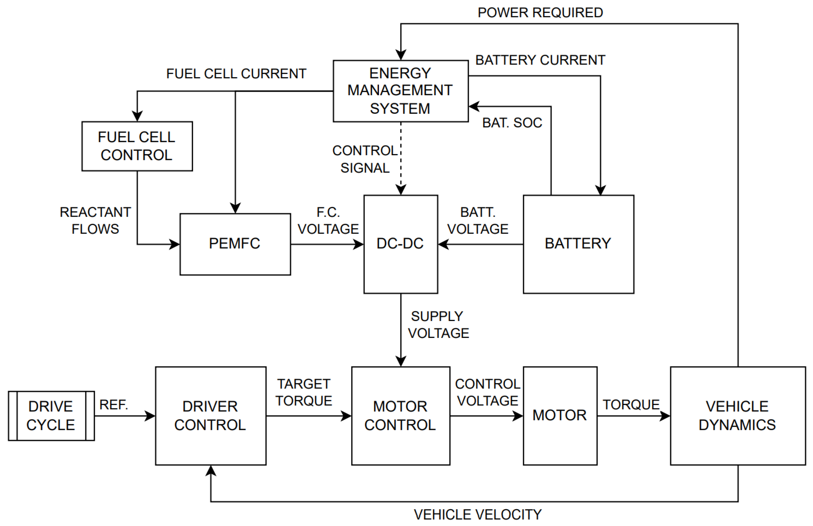
Figure 2.
Example system.
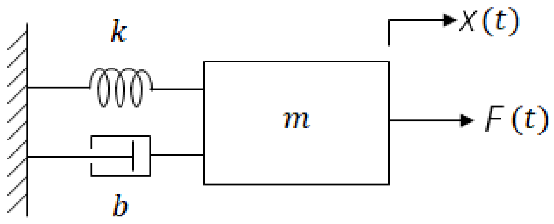
Figure 3.
System model architecture.
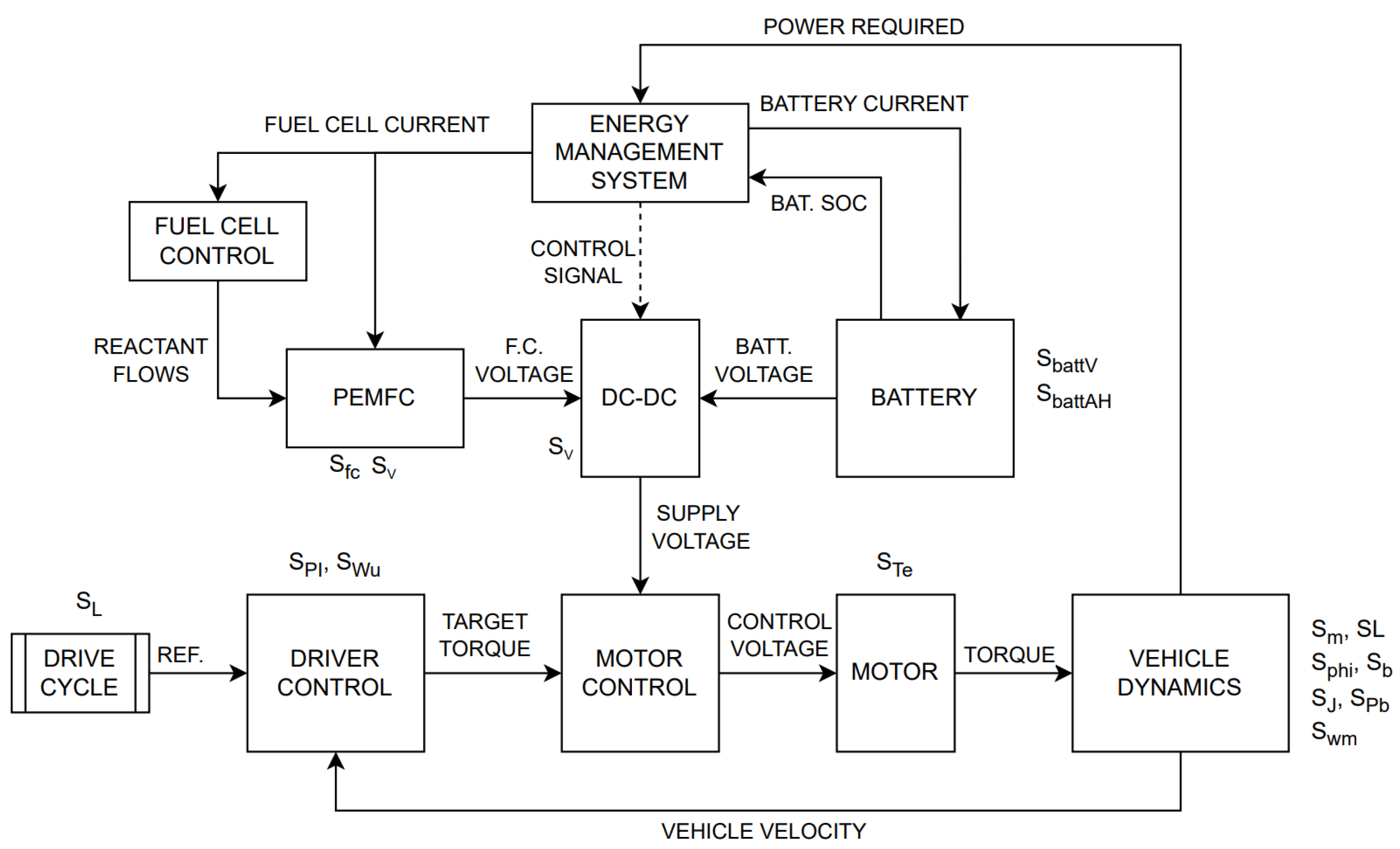
Figure 4.
Linear plant model.
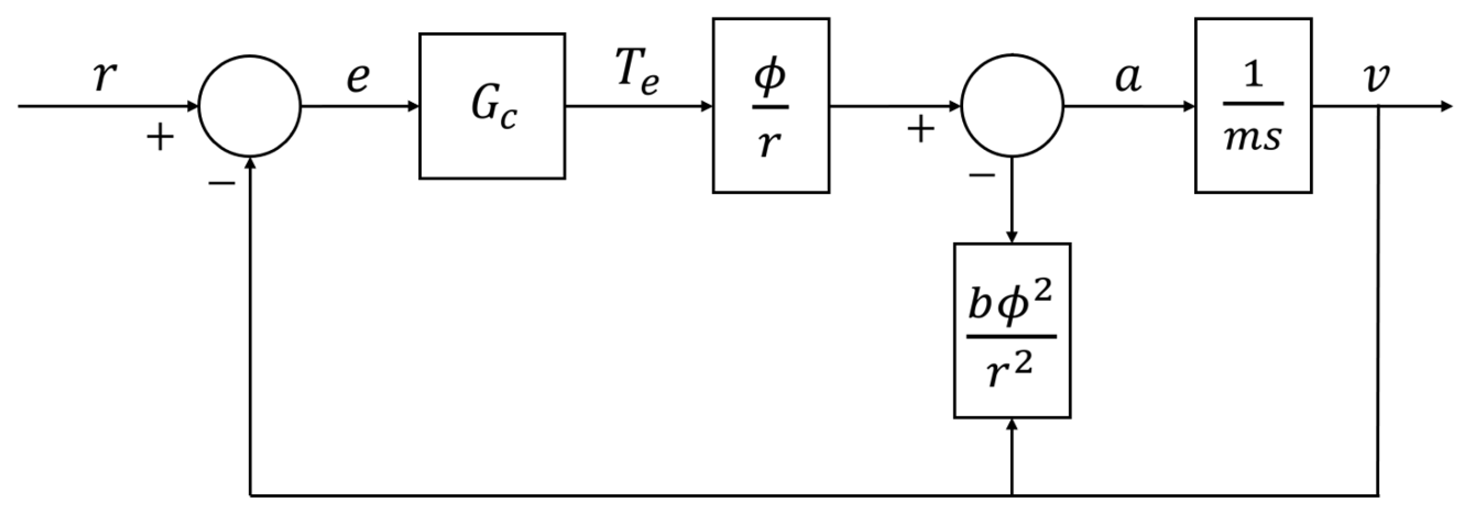
Figure 5.
weighting functions.
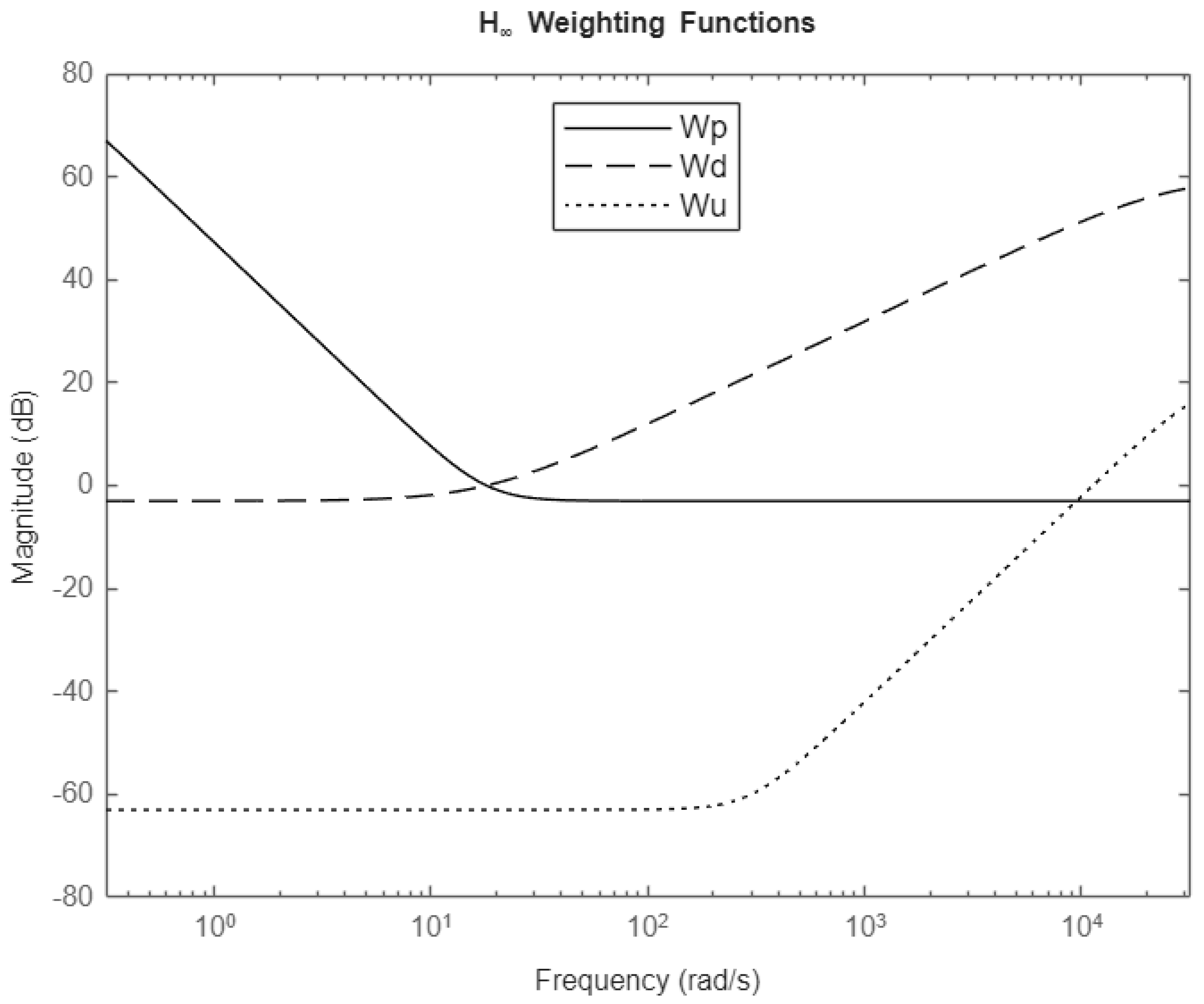
Figure 6.
Bode magnitude and phase plots of the open-loop transfer function L for: (a) Full-scale PI controller. (b) Scaled PI controller.
Figure 6.
Bode magnitude and phase plots of the open-loop transfer function L for: (a) Full-scale PI controller. (b) Scaled PI controller.
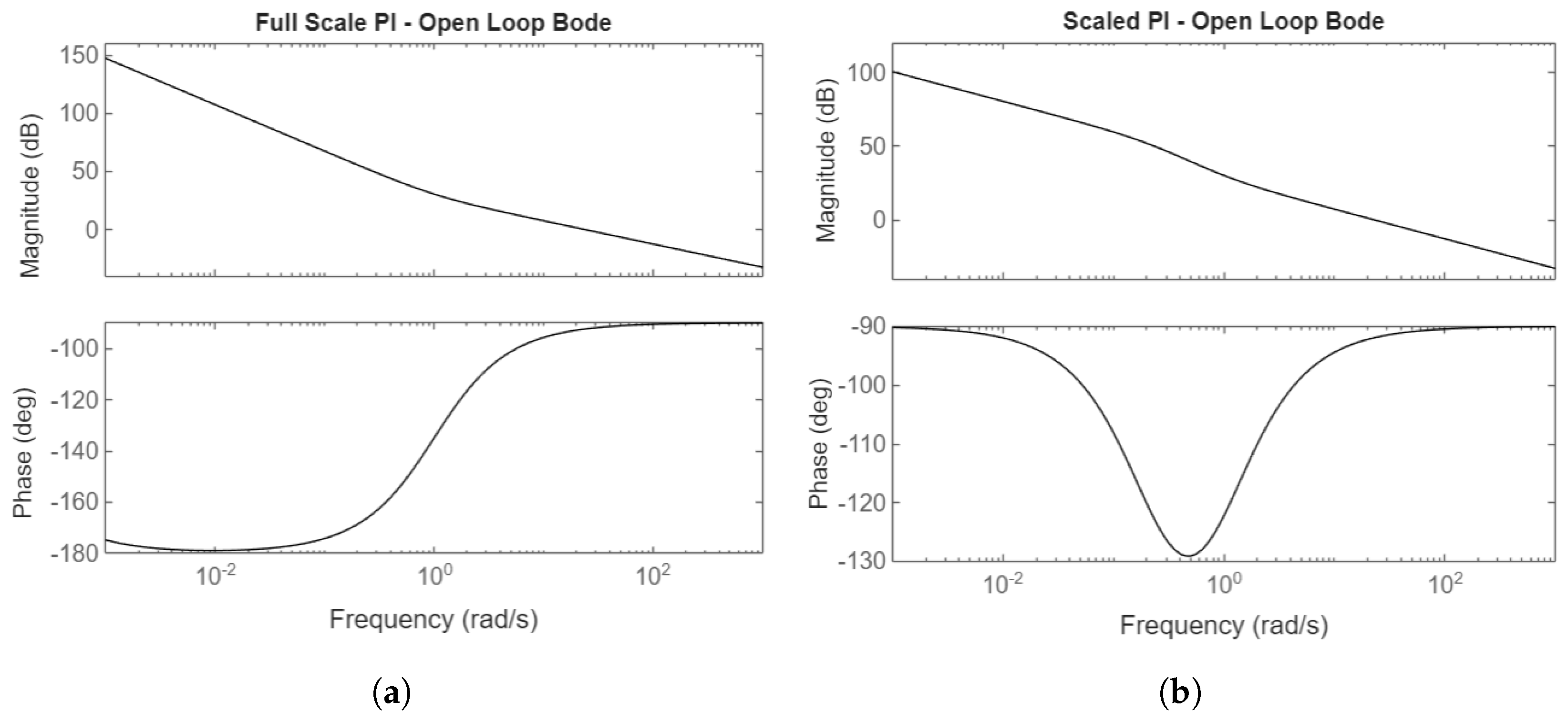
Figure 7.
Bode magnitude and phase plots of the open-loop transfer function L for: (a) Full-scale Youla controller. (b) Scaled Youla controller.
Figure 7.
Bode magnitude and phase plots of the open-loop transfer function L for: (a) Full-scale Youla controller. (b) Scaled Youla controller.
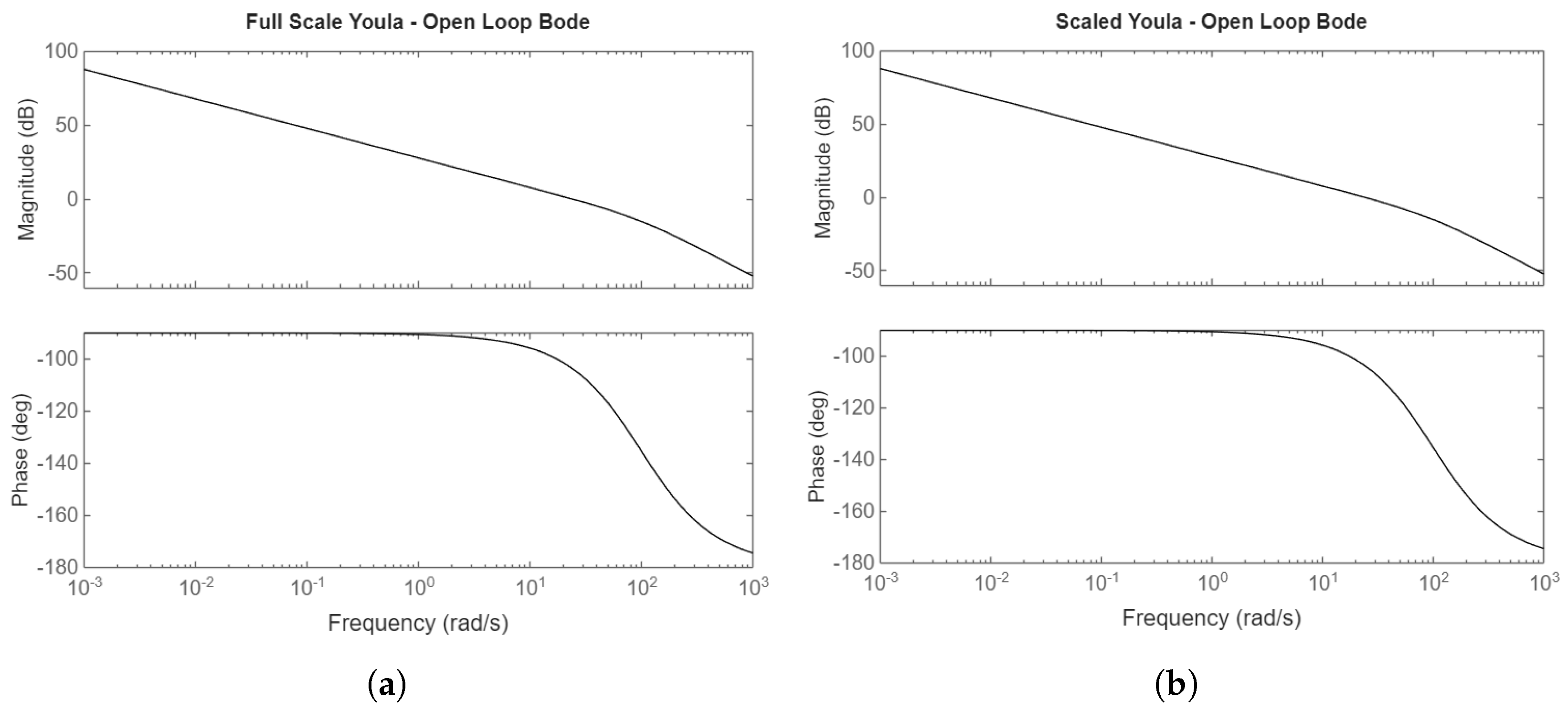
Figure 8.
Bode magnitude and phase plots of the open-loop transfer function L for: (a) Full-scale controller. (b) Scaled controller.
Figure 8.
Bode magnitude and phase plots of the open-loop transfer function L for: (a) Full-scale controller. (b) Scaled controller.
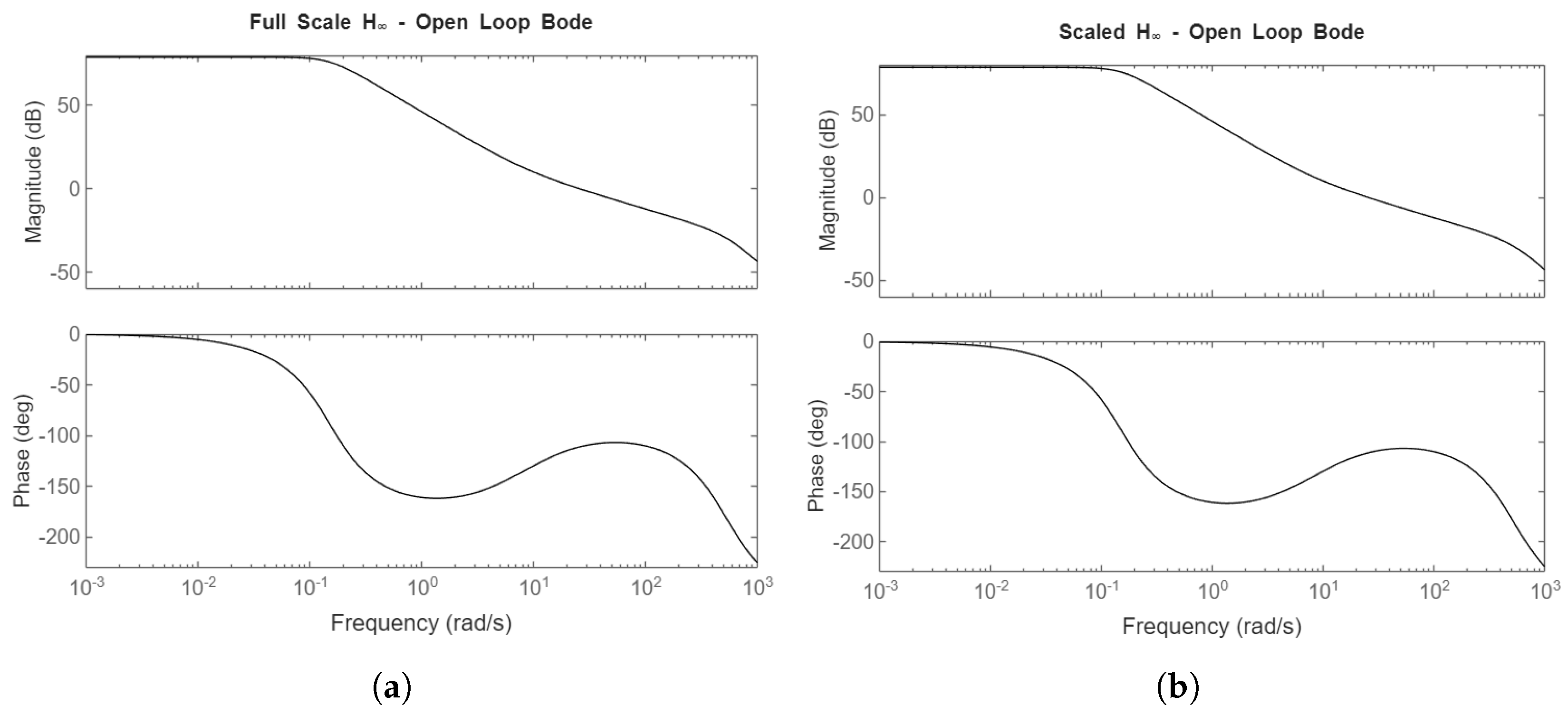
Figure 9.
Bode magnitude and phase plots of the open-loop transfer function L for: (a) Full-scale Youla-H controller. (b) Scaled Youla-H controller.
Figure 9.
Bode magnitude and phase plots of the open-loop transfer function L for: (a) Full-scale Youla-H controller. (b) Scaled Youla-H controller.
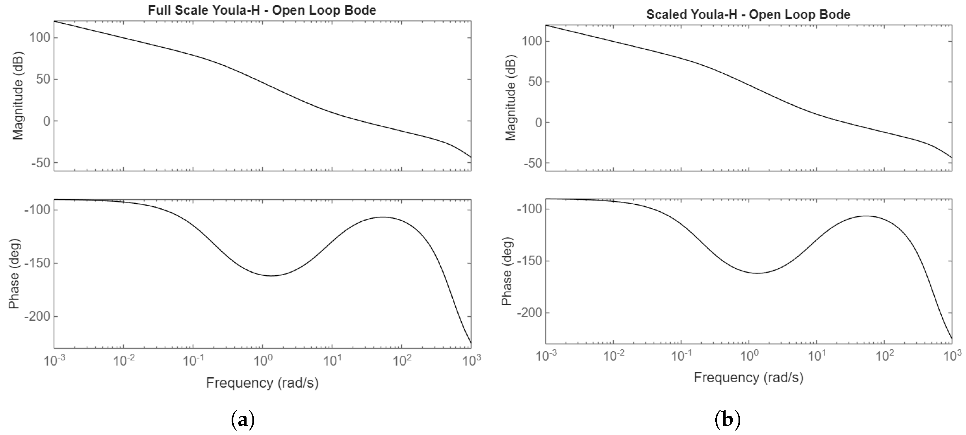
Figure 10.
Bode magnitude plots of the closed-loop transfer functions T, S, and Y for: (a) Full-scale PI controller. (b) Scaled PI controller.
Figure 10.
Bode magnitude plots of the closed-loop transfer functions T, S, and Y for: (a) Full-scale PI controller. (b) Scaled PI controller.
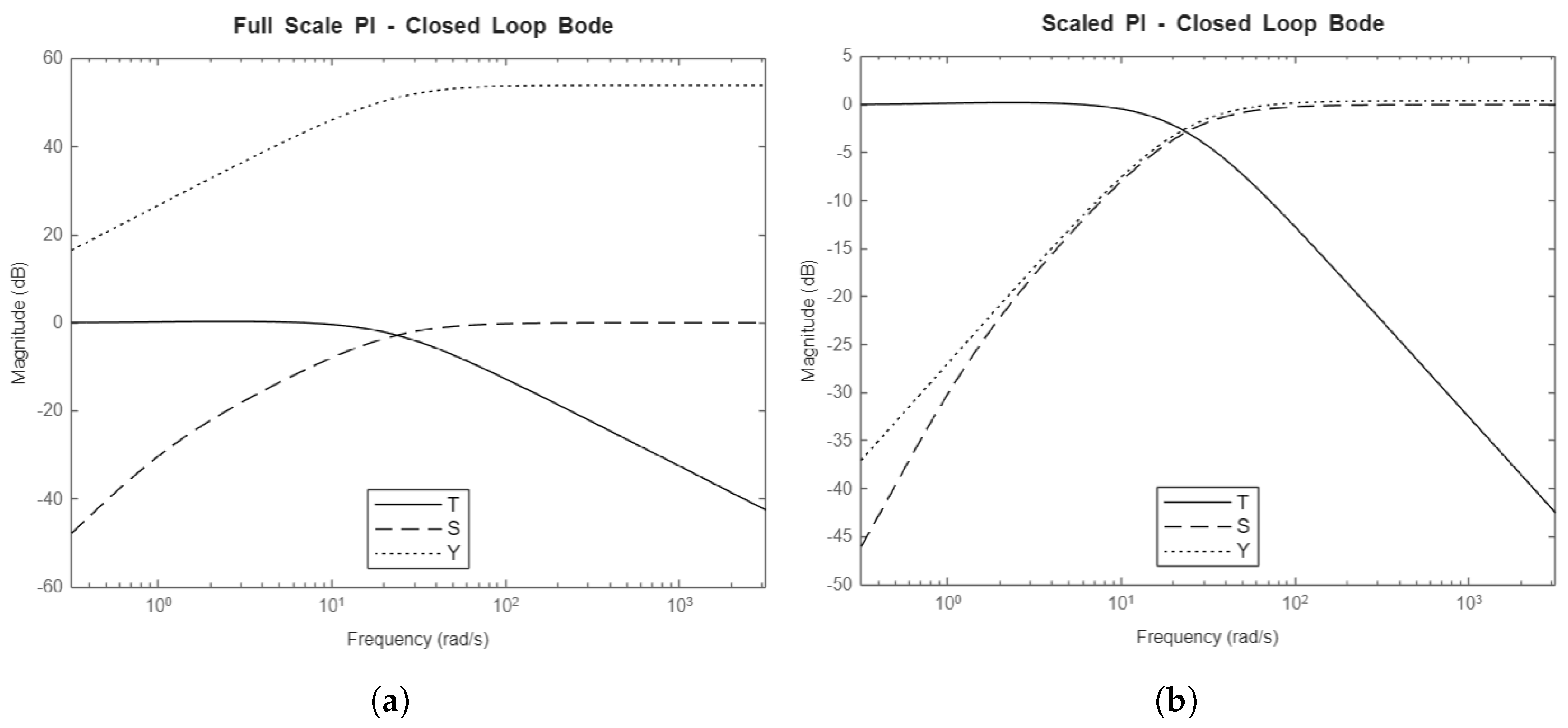
Figure 11.
Bode magnitude plots of the closed-loop transfer functions T, S, and Y for: (a) Full-scale Youla controller. (b) Scaled Youla controller.
Figure 11.
Bode magnitude plots of the closed-loop transfer functions T, S, and Y for: (a) Full-scale Youla controller. (b) Scaled Youla controller.
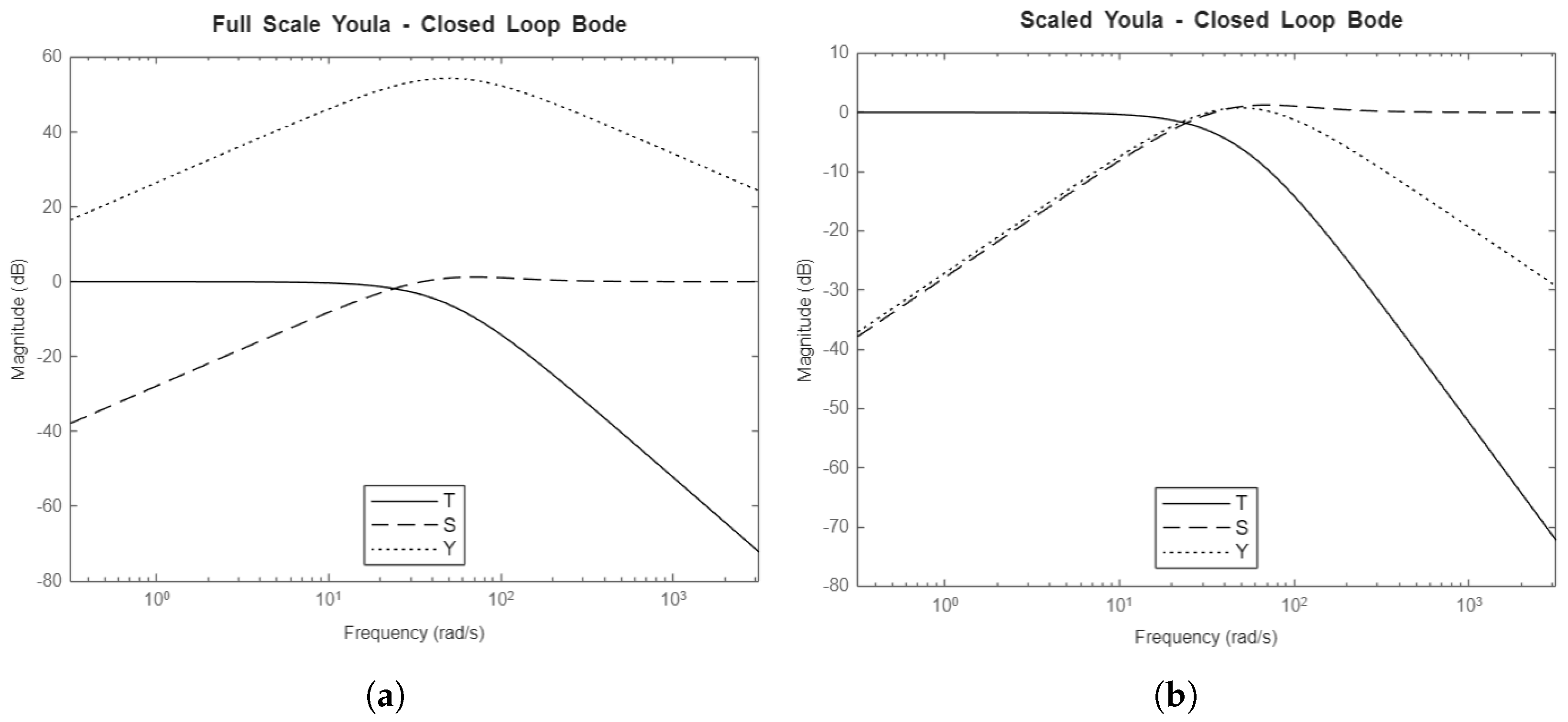
Figure 12.
Bode magnitude plots of the closed-loop transfer functions T, S, and Y, and the inverse of the weighting functions , , and for: (a) Full-scale controller. (b) Scaled controller.
Figure 12.
Bode magnitude plots of the closed-loop transfer functions T, S, and Y, and the inverse of the weighting functions , , and for: (a) Full-scale controller. (b) Scaled controller.
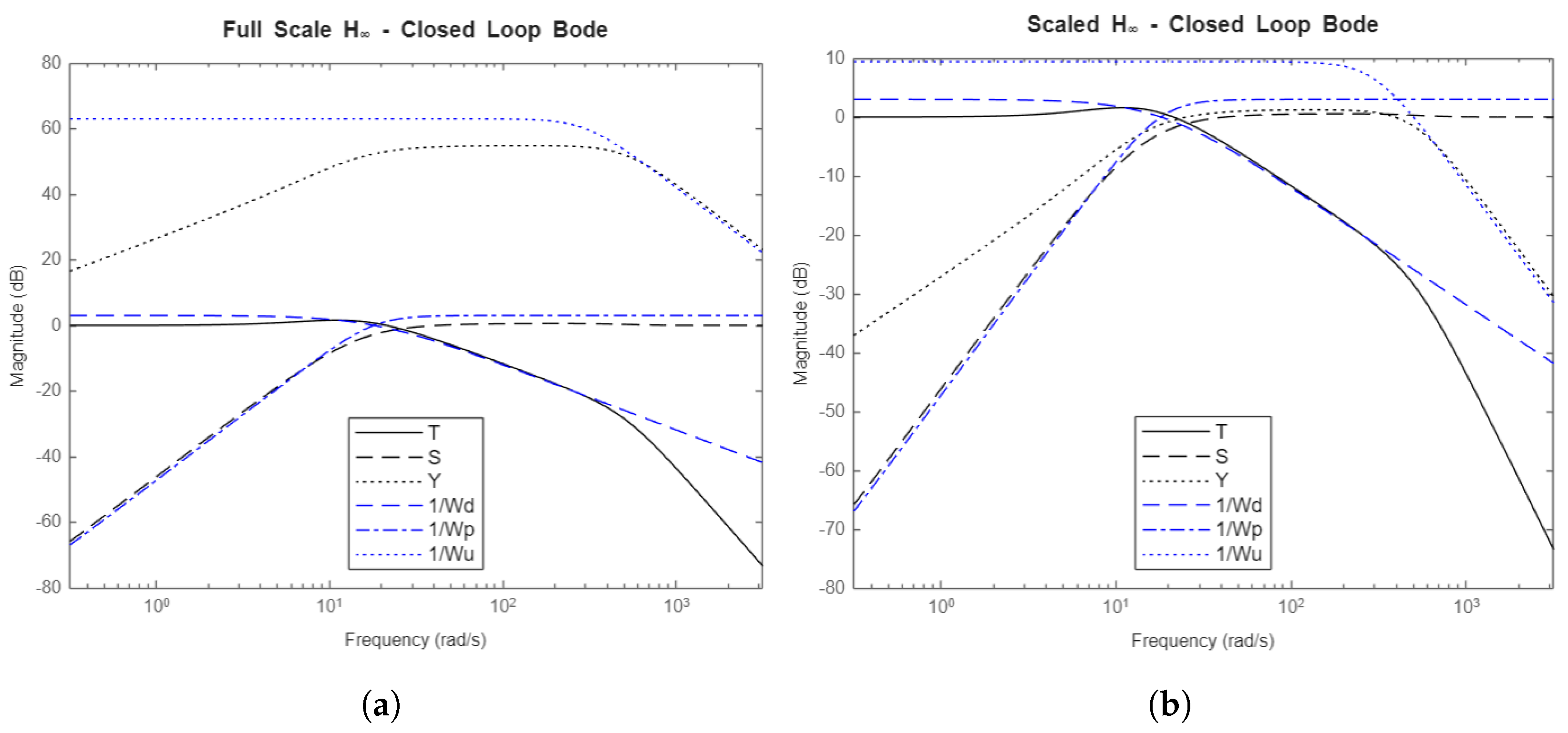
Figure 13.
Bode magnitude plots of the closed-loop transfer functions T, S, and Y for: (a) Full-scale Youla-H controller. (b) Scaled Youla-H controller.
Figure 13.
Bode magnitude plots of the closed-loop transfer functions T, S, and Y for: (a) Full-scale Youla-H controller. (b) Scaled Youla-H controller.
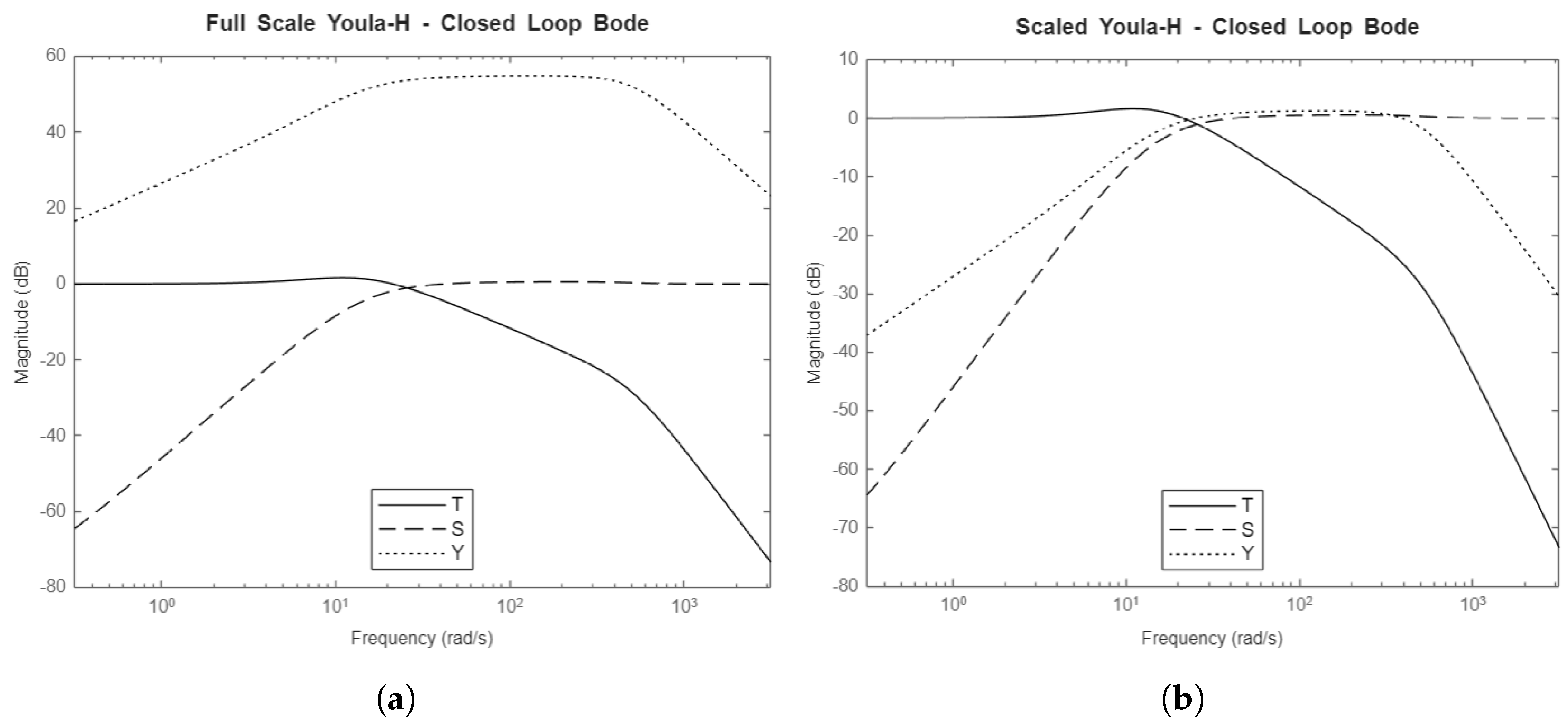
Figure 14.
Nyquist plots for: (a) PI controller. (b) Youla controller. (c) controller. (d) Youla-H controller.
Figure 14.
Nyquist plots for: (a) PI controller. (b) Youla controller. (c) controller. (d) Youla-H controller.
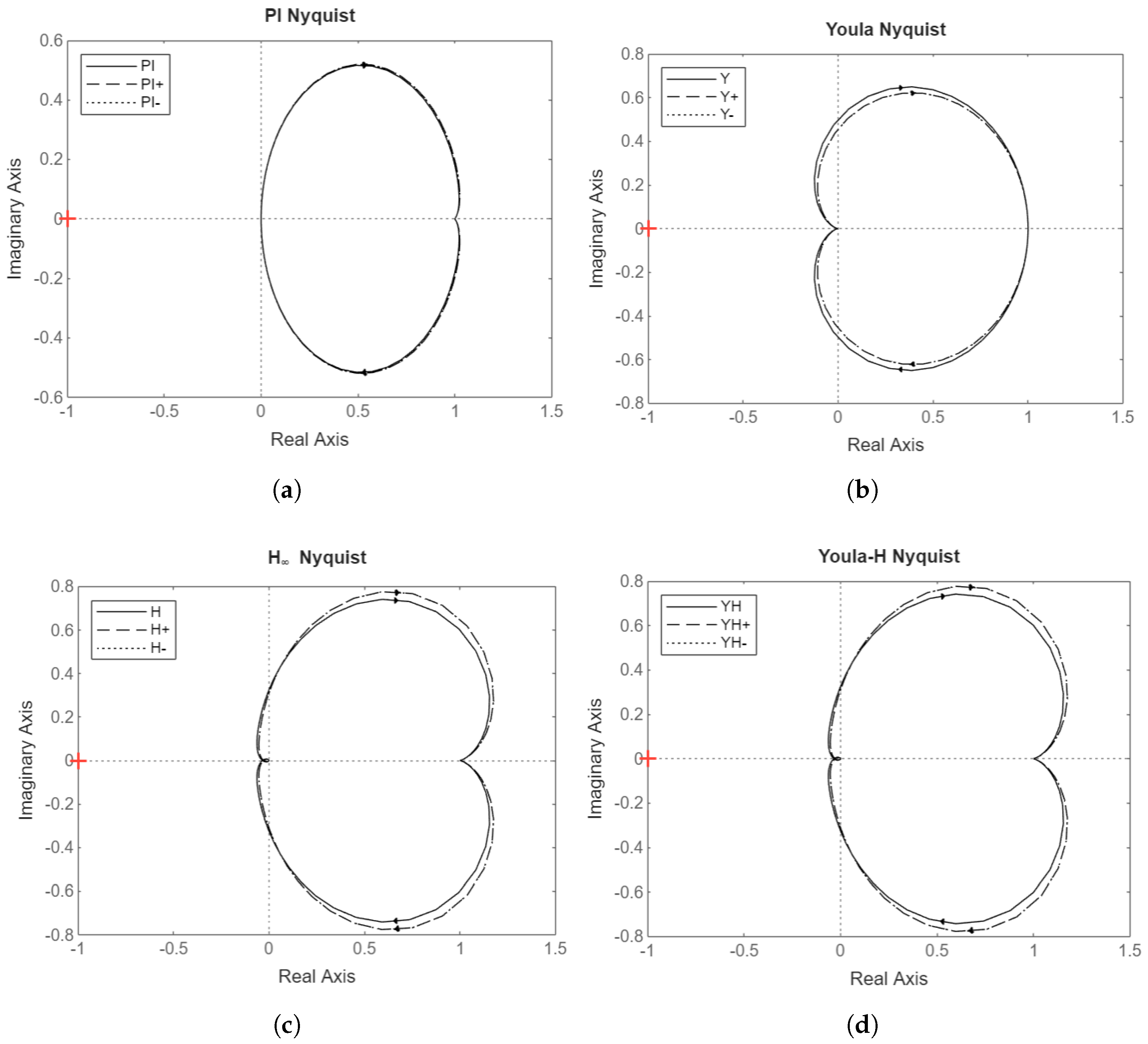
Figure 15.
Linear plant model.
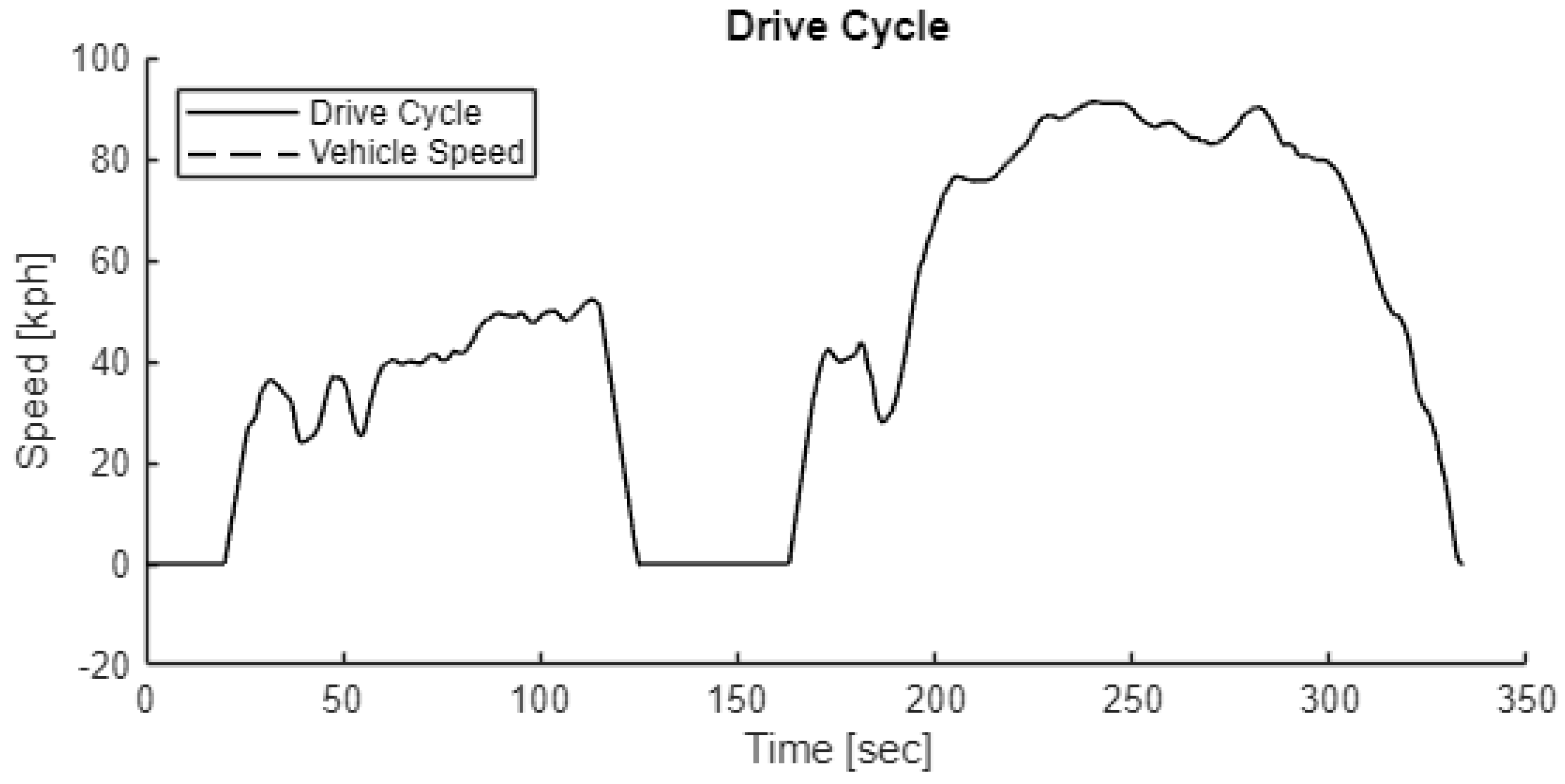
Figure 16.
Normalized tracking errors for: (a) PI controller, full-scale vs scaled. (b) PI controller with parameter variations.
Figure 16.
Normalized tracking errors for: (a) PI controller, full-scale vs scaled. (b) PI controller with parameter variations.
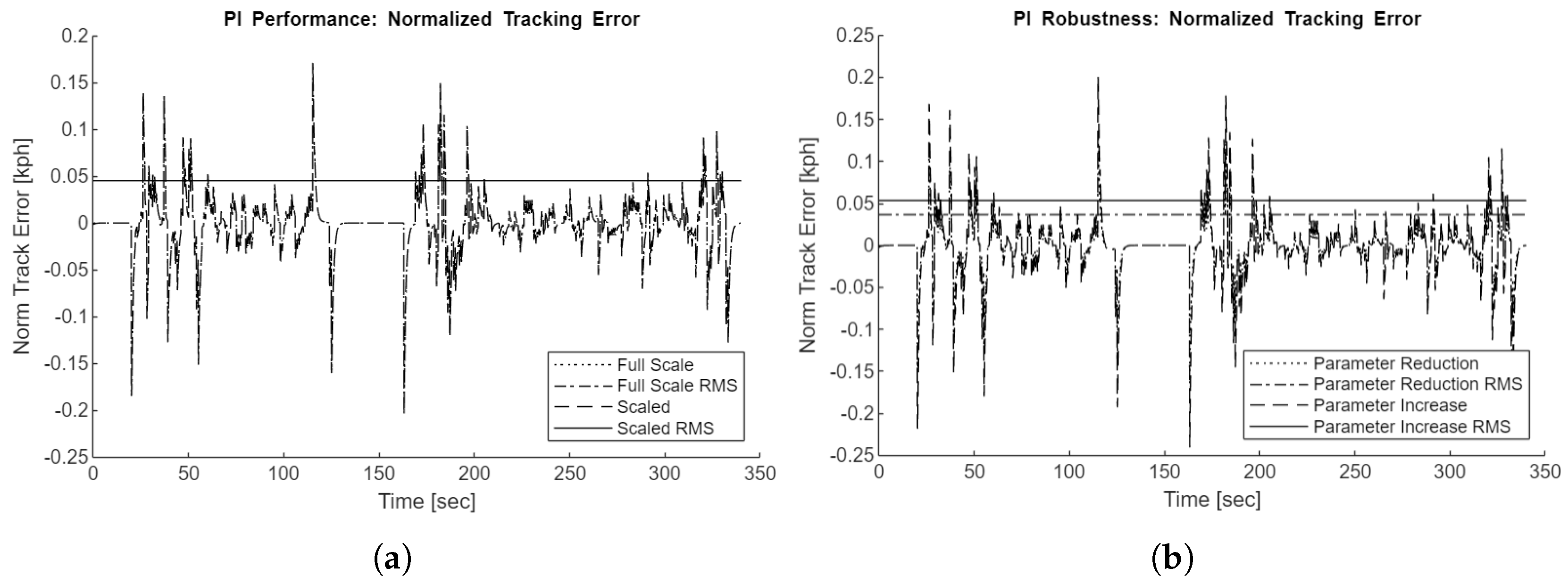
Figure 17.
Normalized tracking errors for: (a) Youla controller, full-scale vs scaled. (b) Youla controller with parameter variations.
Figure 17.
Normalized tracking errors for: (a) Youla controller, full-scale vs scaled. (b) Youla controller with parameter variations.
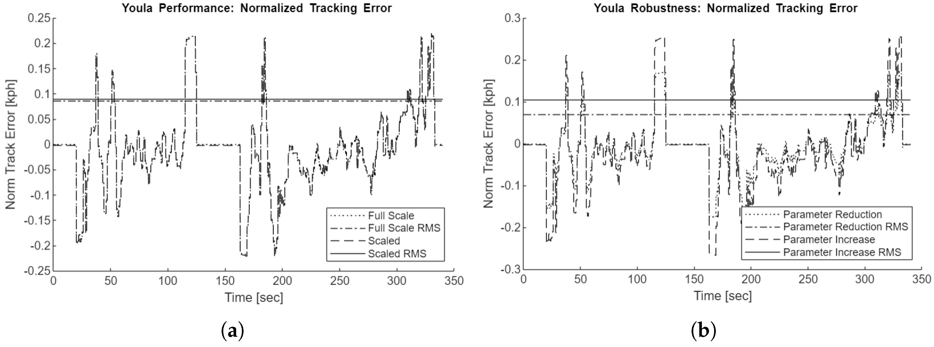
Figure 18.
Normalized tracking errors for: (a) controller, full-scale vs scaled. (b) controller with parameter variations.
Figure 18.
Normalized tracking errors for: (a) controller, full-scale vs scaled. (b) controller with parameter variations.
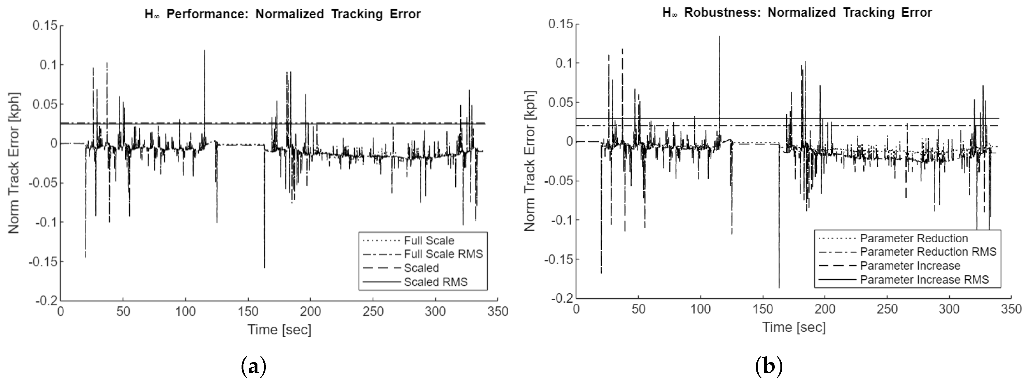
Figure 19.
Normalized tracking errors for: (a) Youla-H controller, full-scale vs scaled. (b) Youla-H controller with parameter variations.
Figure 19.
Normalized tracking errors for: (a) Youla-H controller, full-scale vs scaled. (b) Youla-H controller with parameter variations.
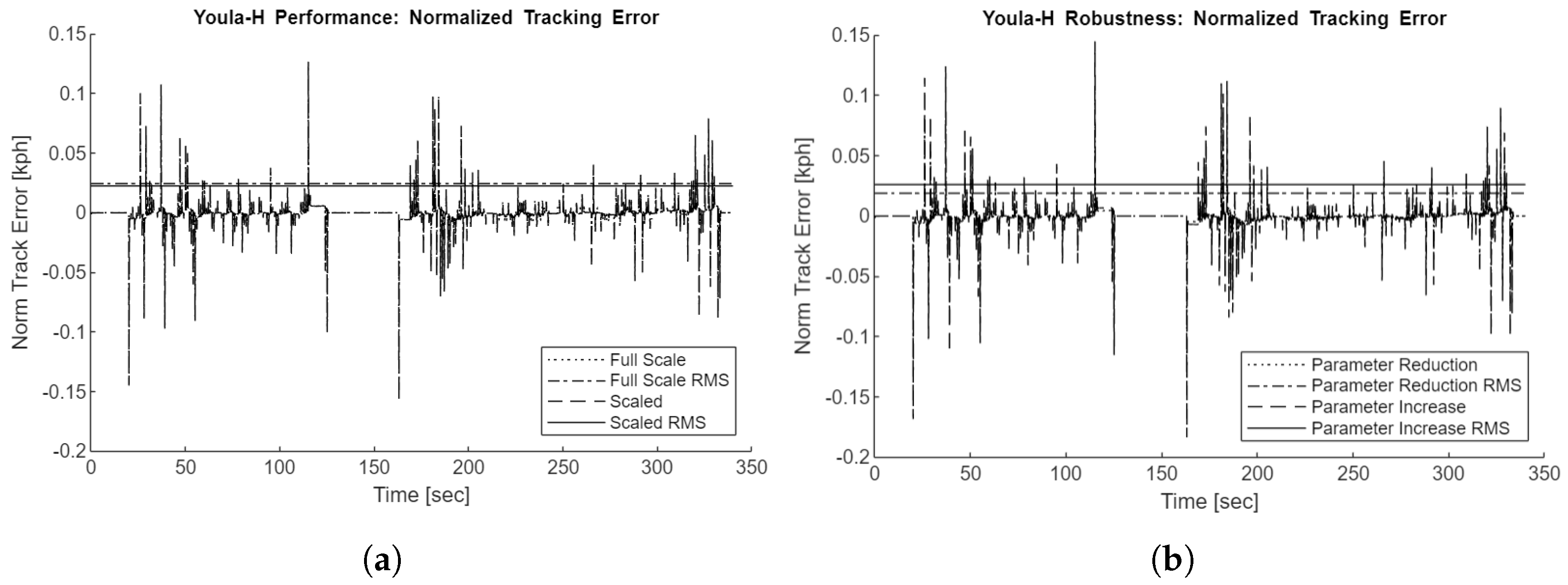
Figure 20.
Actuator effort with noise on the scaled-down plant for: (a) PI controller. (b) Youla controller. (c) controller. (d) Youla-H controller.
Figure 20.
Actuator effort with noise on the scaled-down plant for: (a) PI controller. (b) Youla controller. (c) controller. (d) Youla-H controller.
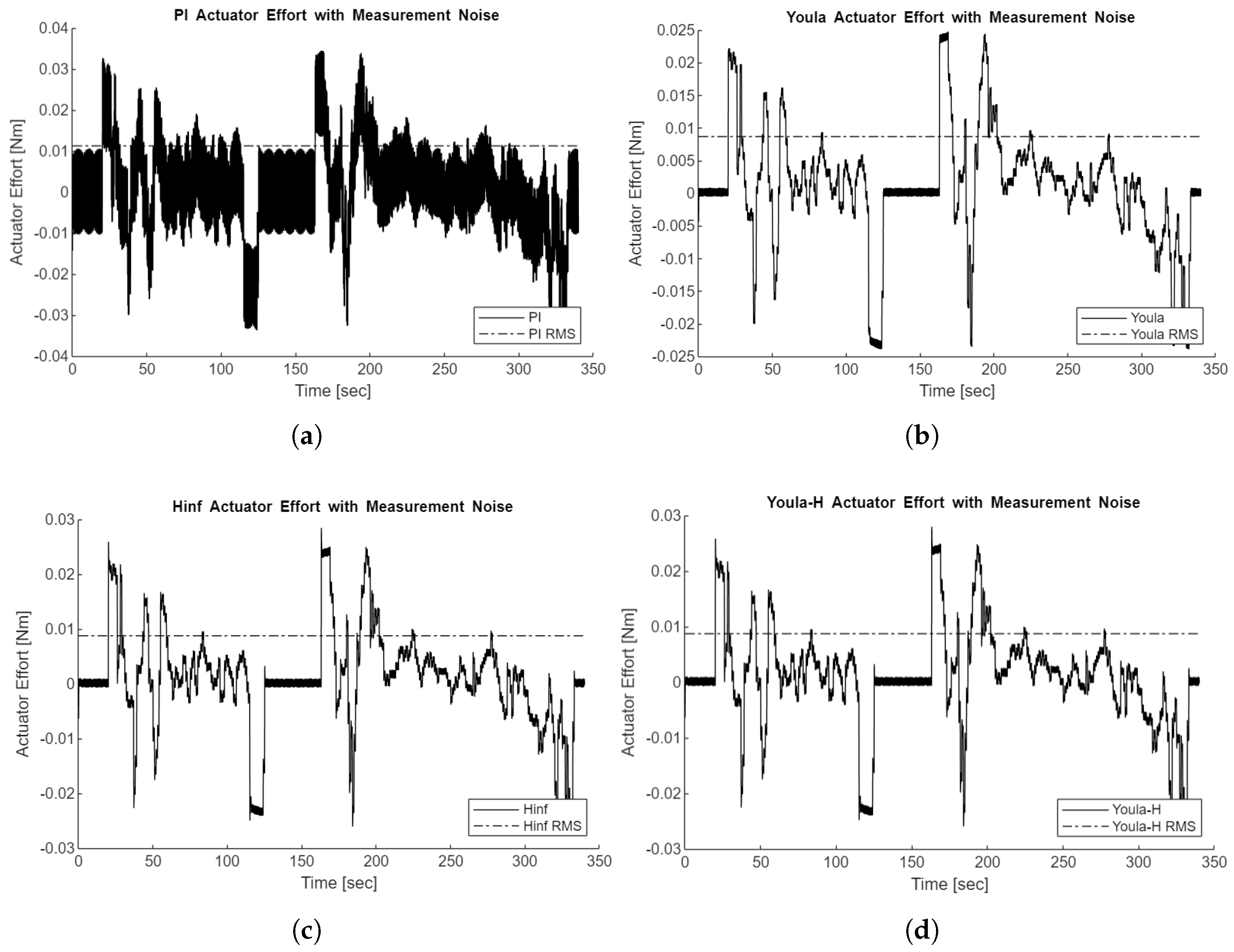

Table 1.
System and Control Parameters.
| Parameters | Scaling | Full Scale Value | Scaled Value | Notes |
|---|---|---|---|---|
| Energy | 1:50,000 | - | - | Independent scaling |
| Length | 1:10 | - | - | Independent scaling |
| Gear Ratio | 1:10.453 | 10.453 | 1 | Independent scaling |
| Efficiency | 1:1 | 95% | 95% | Independent scaling |
| Voltage [V] | 8:720 | 720 | 8 | Independent scaling |
| Mass [kg] | 1:500 | 2,242 | 4.48 | Vehicle mass |
| Force at Wheel [N] | 1:5,000 | - | - | |
| Torque at Wheel [Nm] | 1:50,000 | - | - | |
| Torque at Motor [Nm] | 1:4,784 | 500 | 0.105 | Maximum value |
| Motor Speed [rpm] | 1:10.453 | 21,000 | 2,009 | Maximum value |
| Motor Inertia [kgm2] | 1:458 | 3.50e-2 | 7.65e-5 | |
| Motor Friction [Nm sec/rad] | 1:458 | 1.10e-4 | 2.40e-7 | |
| Braking Pressure [kPa] | 1:50 | 5,000 | 100 | Friction braking only |
| Proportional Gain [1/kph] | 10:1 | 1.0 | 10 | Outputs normalized torque |
| Integral Gain [1/kph] | 10:1 | 1.0 | 10 | Outputs normalized torque |
| Feedforward Gain [1/kph] | 10:1 | 0.001 | 0.01 | Outputs normalized torque |
| Weighting [m/Nm] | 478:1 | 0.001 | 0.478 | Cost function weight |
Table 2.
Maximum Absolute Tracking Errors.
| Max Error [kph] | PI | Youla | Youla-H | |
|---|---|---|---|---|
| Full-Scale | 0.203 | 0.220 | 0.157 | 0.156 |
| Scaled | 0.203 | 0.221 | 0.158 | 0.156 |
| Scaled-Reduction | 0.164 | 0.179 | 0.135 | 0.134 |
| Scaled-Increase | 0.241 | 0.264 | 0.187 | 0.184 |
Table 3.
Root-Mean-Square Tracking Errors.
| RMS Error [kph] | PI | Youla | Youla-H | |
|---|---|---|---|---|
| Full-Scale | 0.045 | 0.086 | 0.026 | 0.024 |
| Scaled | 0.045 | 0.089 | 0.025 | 0.023 |
| Scaled-Reduction | 0.037 | 0.069 | 0.020 | 0.019 |
| Scaled-Increase | 0.054 | 0.105 | 0.029 | 0.026 |
Table 4.
Controller Performance Metrics.
| Metric | PI | Youla | Youla-H | |
|---|---|---|---|---|
| Max Error Nominal [kph] | 0.203 | 0.221 | 0.158 | 0.156 |
| Max Error Reduced Param % | -19.0% | -19.0% | -14.7% | -14.4% |
| Max Error Increased Param % | 18.6% | 20.6% | 18.0% | 17.6% |
| RMS Error Nominal [kph] | 0.045 | 0.089 | 0.025 | 0.023 |
| RMS Error Reduced Param % | -19.2% | -22.4% | -18.2% | -16.4% |
| RMS Error Increased Param % | 18.1% | 16.9% | 18.2% | 15.6% |
| M2 Margin | 1.000 | 0.866 | 0.937 | 0.937 |
| Noise Std. Dev. [Nm] | 0.0071 | 0.0005 | 0.0005 | 0.0005 |
| Noise Max [Nm] | 0.0142 | 0.0043 | 0.0063 | 0.0063 |
Disclaimer/Publisher’s Note: The statements, opinions and data contained in all publications are solely those of the individual author(s) and contributor(s) and not of MDPI and/or the editor(s). MDPI and/or the editor(s) disclaim responsibility for any injury to people or property resulting from any ideas, methods, instructions or products referred to in the content. |
© 2025 by the authors. Licensee MDPI, Basel, Switzerland. This article is an open access article distributed under the terms and conditions of the Creative Commons Attribution (CC BY) license (http://creativecommons.org/licenses/by/4.0/).
Copyright: This open access article is published under a Creative Commons CC BY 4.0 license, which permit the free download, distribution, and reuse, provided that the author and preprint are cited in any reuse.


