
Submitted:
02 May 2025
Posted:
05 May 2025
You are already at the latest version
Abstract
This study presents a comprehensive analysis of CO₂ trapping mechanisms in reservoirs, integrating reservoir simulations, geochemical modeling, and machine learning techniques to enhance the understanding of carbon capture and storage (CCS). A 2D reservoir model was developed to simulate CO₂ injection dynamics, incorporating various trapping mechanisms: residual, solubility, mineralization, and structural, under realistic geomechanical and geochemical conditions. Advanced machine learning models, including Random Forest, Gradient Boosting, and Decision Trees, were employed to act as Smart Proxy models, significantly reducing computational time while maintaining predictive accuracy. Results highlight the critical role of hysteresis and aquifer dynamics in enhancing trapping efficiency and long-term CO₂ storage stability. The study underscores the potential of combining traditional reservoir engineering methods with machine learning-driven analytics to optimize CCS strategies, ensuring sustainable and secure storage solutions.
Keywords:
Carbon Capture and Storage
; Carbon Dioxide
; Smart Proxy Model
; Machine Learning
; Decision Tree
; Random Forest
; Peng-Robinson Equation of State
1. Introduction
The magnitude of CO₂ emissions generated by oil and gas operations is substantial, with total global energy-related CO₂ emissions reaching approximately 36.8 billion tonnes (Gt) in 2022, emphasizing the significant contribution of the oil and gas sector to worldwide greenhouse gas emissions [1]. In recent years, there has been a significant increase in awareness and concern about the continuous buildup of greenhouse gases in our atmosphere. This buildup is primarily driven by human activities such as fossil fuel combustion, deforestation, and industrial processes that release greenhouse gases like carbon dioxide (CO₂), methane, and nitrous oxide [2]. The rising concentration of these gases has contributed to global temperature increases, triggering significant climate changes that pose a serious threat to the planet [3]. In 2022, these activities contributed roughly 15% of global energy-related emissions, amounting to an estimated 5.1 billion tonnes of greenhouse gases [4]. This significant contribution to global emissions highlights the critical need for action within this sector. The adoption of the Paris Agreement in 2015 was a landmark moment in global climate efforts, establishing ambitious goals to limit global warming to well below 2°C above pre-industrial levels, with an emphasis on striving to restrict the increase to 1.5°C [5]. As countries work toward meeting these climate goals, carbon dioxide (CO₂) storage has become a crucial tool in combating climate change. Carbon capture and storage (CCS) technology has the capability to eliminate 90-99% of CO₂ emissions from industrial sources, making it an essential solution for decarbonizing hard-to-abate sectors and supporting nations in fulfilling their climate commitments [6]. The 2023 COP28 conference in Dubai reinforced the urgency of addressing climate change, highlighting the need to expedite the transition to clean energy and significantly increase climate financing efforts [7]. The conference underscored the critical role of innovative technologies such as CCS in achieving the Paris Agreement goals, emphasizing that sustained government backing and international collaboration are essential for unlocking the full potential of CO₂ storage in the fight against global warming [8].
Field tests have traditionally played a crucial role in evaluating the feasibility and performance of CO₂ storage in subsurface formations. These tests, often conducted at pilot or demonstration sites, provide valuable insights into reservoir behavior, injectivity, plume migration, and trapping mechanisms under real conditions [9,10]. Notable examples include the Sleipner and Snøhvit projects in Norway [11,12,13], which have offered decades of observational data. While field tests offer high-fidelity results and ground-truth validation, they are typically time-consuming, expensive, and limited in spatial and temporal resolution. In contrast, reservoir simulations offer a more cost-effective and flexible approach to studying a wide range of reservoir conditions and scenarios.
Reservoir simulations help predict how CO₂ will spread, interact with rock and fluids, and become trapped within the reservoir. These models provide critical insights into the movement of CO₂ plumes over time, enabling engineers to assess storage capacity, evaluate seal integrity, and identify potential risks such as leakage or pressure build-up. By simulating complex geological conditions and fluid behaviors, reservoir simulations aid in optimizing injection strategies, ensuring efficient utilization of storage space, and enhancing the long-term safety and reliability of carbon storage projects. Additionally, they play a key role in validating monitoring plans and supporting regulatory compliance, contributing to the overall success of carbon capture and storage (CCS) initiatives. As noted by [14], "Reservoir simulation is a direct numerical modelling method to model fluid flow in a reservoir or in a better description in the porous medium”. These simulations can represent various trapping mechanisms, such as structural, residual, solubility, and mineral trapping, each functioning over different time scales [15].
In this study, we developed a base reservoir model to simulate CO₂ injection in a grid containing a centrally located injection well, flanked by two production wells positioned on either side. This well arrangement was chosen to examine the influence of nearby production wells on the reservoir's pressure distribution, CO₂ saturation levels, injectivity, and trapping efficiency under varying geomechanical and geochemical conditions. This setup facilitates a thorough assessment of CO₂ storage behavior within a more realistic reservoir configuration, offering insights into the complex interactions affecting CO₂ containment and mobility in subsurface storage projects[16]. The complexity of the base model was incrementally tuned with each new set of simulations, enabling the characterization of specific trapping mechanisms. We began by simulating hysteresis and residual gas trapping to understand their roles in CO₂ immobilization. Subsequently, we incorporated an infinite-acting aquifer into the model to assess its impact on pressure distribution, flow patterns, CO₂ plume behavior, saturation levels, and overall trapping efficiency in the reservoir. CMG Builder was used to build the 2-dimensional Grid, WinProp which is CMG’s equation of state multiphase equilibrium property package was used for fluid component characterization.
In this study, advanced machine learning algorithms were employed as smart proxy models (SPMs) to enhance the efficiency and accuracy of reservoir simulations. SPMs serve as simplified, data-driven approximations of complex numerical models, capturing the essential relationships between key reservoir parameters and outputs [17]. Incorporating SPMs into reservoir simulation is particularly beneficial for several reasons. First, SPMs allow for rapid evaluation of multiple scenarios, enabling engineers to explore a wide range of conditions, including various injection strategies and reservoir properties, in a fraction of the time needed for full-scale numerical modeling [18]. Additionally, SPMs facilitate the integration of uncertainty analysis by enabling repeated runs over large parameter spaces without overwhelming computational resources. This capability is vital for understanding the sensitivity of reservoir performance to key variables, improving the robustness and reliability of predictions. The use of SPMs also democratizes access to advanced modeling by reducing the technical and computational barriers, making it easier for teams with limited resources to engage in high-quality reservoir analysis. By combining machine learning with traditional numerical methods, this approach enhances the scalability, flexibility, and applicability of reservoir simulations, ultimately supporting more efficient and effective management of subsurface storage projects. The integration of SPMs into this study highlights the transformative potential of machine learning in numerical modeling, providing a pathway to faster, more cost-effective, and equally reliable results in reservoir engineering and beyond. As demonstrated by [18], Smart Proxy Models can replicate numerical simulations with high accuracy and can be run on a laptop within minutes, simplifying the use of complex numerical simulations that might otherwise take tens of hours.
2. Materials and Methods
In this study, three advanced machine learning models were utilized: Random Forest, Gradient Boosting, and Decision Trees. These models were deployed as intelligent proxy models to enhance the efficiency and accuracy of predicting the volume of CO₂ trapped within the reservoir. The primary motivation behind using these models was to significantly reduce the simulation and computational time required for analyzing large datasets, while maintaining robust predictive capabilities. By leveraging these machine learning approaches, the study aimed to capture the complex, nonlinear relationships inherent in the simulation results obtained from CO₂ injection scenarios. The models were trained and validated using data generated from simulations, ensuring their ability to generalize across various conditions. Additionally, these proxy models provided insights into key reservoir parameters influencing CO₂ trapping, enabling faster decision-making and optimization of injection strategies.
2.1. Random Forest
The Random Forest algorithm operates on the principle of ensemble learning, specifically using a technique called bagging (bootstrap aggregating). RF creates multiple decision trees by randomly sampling the training data with replacement. This process is called bootstrap sampling. At each node of a decision tree, RF selects a random subset of features to consider for splitting. This introduces additional randomness and helps to decorrelate the trees [19]. At each split node, a binary test is conducted on a subset, directing the result to either the left or right sub-node. The test involves selecting a random subset of features and identifying a value that minimizes the mean square error , to determine the optimal branch. This process can be represented as:
Here, Ei represents the true value of the i-th sample, while C1 and C2 denote the predicted values for the left and right subspaces, D1 and D2, respectively. Each tree is grown to its maximum depth or until a stopping criterion is met. The trees are not pruned, allowing them to capture complex patterns in the data. For regression tasks, the average prediction of all trees is used as shown below:
The combined regression model is depicted as f(x)
RF can capture complex, non-linear relationships in the data, which is crucial for modeling complex systems like oil and gas reservoirs. RF provides a measure of feature importance, helping to identify the most influential parameters in the model [13]. Random Forest regression algorithms have been employed to predict CO2-WAG (Water-Alternating-Gas) performance, including oil production, CO2 storage amount, and storage efficiency which just reiterates its usage as a smart proxy model as seen in [14]
2.2. Gradient Boosting
The model starts with an initial prediction, often the mean of the target variable for regression tasks. In each iteration, the model calculates the residuals (differences between predictions and actual values) [20]. A new weak learner (e.g., a decision tree) is trained to predict these residuals. The predictions of this new learner are added to the ensemble's predictions, scaled by a learning rate. The algorithm aims to minimize a specified loss function (e.g., mean squared error for regression) at each step, by iteratively reducing the loss, the model improves its predictive accuracy. Various techniques like shrinkage (learning rate) and subsampling are used to prevent overfitting.
2.3. Decision Trees
A decision tree consists of nodes (decision points) and branches (possible outcomes). The topmost node is called the root node, internal nodes represent features, and leaf nodes represent the final decisions or predictions as shown in Figure 1 below. Each node evaluates a feature and splits the dataset based on a threshold value. The objective is to maximize the homogeneity of resulting subsets or minimize the loss function (e.g., mean squared error for regression). The dataset is split recursively based on feature values that optimize a chosen metric.
Common splitting metrics include:
- Gini Impurity: Measures the probability of incorrect classification of a randomly chosen element.
- Entropy (for information gain): Measures the disorder or uncertainty in the dataset.
- Variance Reduction: Used in regression tasks to minimize variance within subsets.
To prevent overfitting, trees can be pruned by removing branches that provide little predictive power. Decision tree-based models have been used to predict CO2 solubility in aqueous solutions, which is crucial for understanding CO2 behavior in reservoirs as seen in [21]. Decision tree algorithms and their ensemble variants offer a powerful and interpretable approach to modeling complex CO2 injection scenarios. Their ability to capture non-linear relationships, provide feature importance, and make rapid predictions makes them valuable tools for developing smart proxy models in reservoir simulation and optimization [22].
2.4. Base Case Model
The base model was developed using CMG’s software packages: Builder, GEM, and WinProp to create a Cartesian grid with dimensions of 100 blocks in the i-direction, 1 block in the j-direction, and 20 blocks in the k-direction, as outlined in Table 1. Each layer in the k-direction has a thickness of 5 meters, with the top of the grid starting at 1200 meters, giving the reservoir a total thickness of 100 meters, extending from 1200m at the top to 1300m at the bottom as seen in Figure 3 below. The reservoir was modeled with isotropic permeability, meaning permeability values are consistent in all directions, and a uniform single porosity of 18% throughout. All measurements in this study adhere to S.I. units. The reservoir pressure and temperature were set at 11,800 kPa and 50°C, respectively.
For the base case simulation, the Peng Robinson Equation of State (PR EOS) [19] was applied, as shown in Equation 3-1. The PR EOS establishes a relationship between thermodynamic properties and phase equilibrium for CO₂, determining densities, fugacities, and equilibrium phase compositions based on input conditions. This model also incorporates a generalized equation of state for pure components in GEM, as presented in Equation 3-2. The reservoir fluid components were modeled in WinProp with carbon dioxide (CO₂) indicated as the Secondary component, being the injection fluid. However, Methane (CH₄) is specified as a primary component and reservoir fluid with a mole fraction composition of 0.999 but is treated as a trace component by the simulator to maintain a gas phase in each block. The inclusion of methane as a trace component is essential for initializing aqueous solubility equations across the blocks. It ensures that a minimal amount of gas is present for phase calculations without allowing methane to dissolve in water, thereby facilitating accurate gas property calculations. The Rowe-Chou aqueous density correlation and the Kestin aqueous viscosity correlation were chosen as the recommended correlations for aqueous density and viscosity calculations for CCS simulations.
Water gas contact was set at 1150m which indicates that the whole reservoir is under water. Injection time was set at 10 years from the year 2024, after which the well is shut-in while monitoring was carried out for 40 additional years post injection making a total of 50 years. The constraints governing the operation of the injection well and producer wells are detailed in Table 2 below.
2.5. Residual Gas Trapping
This hysteresis simulation was a two phase hysteresis based on Carlson and Land’s model. This trapping mechanism, a physical process of CO₂ immobilization, relies on CO₂ movement and interaction with the aqueous phase, governed by saturation hysteresis and capillary forces. Relative permeability, which defines the ease with which a phase moves through the porous medium, depends on various rock and fluid properties, including wettability, flow rate, interfacial tension, and saturation history[20]. During CO₂ injection, the flow initially aligns with the relative permeability drainage curve for gas, as shown in Figure 3. Upward CO₂ migration results from convective currents and gravity differentials between CO₂ and brine. This migration reduces water saturation near the injection well, followed by an increase in water saturation as the CO₂ plume moves away. This increase causes a transition from drainage to imbibition, altering the gas flow path as graphically depicted in Figure 4 below. KrgD referes to the drainage curve while KrgI refers to the imbibition curve. These curves govern the working principle of the Land’s method in the model. The input Krg values put into the simulator is automatically generates a curve recognized as a drainage curve by the simulator. Through hysteresis, CO₂ trapping occurs as residual gas saturation shifts from the drainage to the imbibition phase, reducing CO₂ mobility[21]. This shift minimizes the risk of CO₂ migrating towards upper reservoir layers, enhancing gas containment within the storage formation [22,23]. This trapping mechanism, often referred to as residual or hysteresis trapping, is vital for secure, long-term CO₂ sequestration. Hysteresis was activated in the model with an Sgt,max value of 0.4. Equations (3) and (4) above illustrate the underlying parameters that influence Land’s model, which assists in predicting drainage curves accurately.
2.6. Hysteresis with Infinite Acting Aquifer
At this stage of the simulation, to simulate the presence of an infinite-acting aquifer, we applied a pore volume multiplier to expand the size of the lowest reservoir layer, as illustrated in Figure 5. By increasing the volume in this region, the model can simulate the effects of an endless water influx from an aquifer, allowing for more realistic analysis of pressure behavior, saturation changes, and fluid movement over time. The increased volume in the aquifer region effectively supports the surrounding layers, replicating how an infinite aquifer would behave in a real-world scenario by continuously supplying water to maintain reservoir pressure. This approach effectively mimics the characteristics of an infinite aquifer, allowing us to observe how this additional water influx would impact reservoir conditions over time. We analyzed key parameters, including changes in pressure, water saturation, gas saturation, and gas density across different time intervals. This setup enabled a detailed investigation into how the aquifer’s influence alters reservoir dynamics, providing insights into fluid flow, gas migration, and pressure maintenance throughout the simulation.
2.7. Solubility Trapping
In this study, our solubility simulations were based on Henry’s Law and Harvey’s correlation [25]. According to Henry’s Law, at a constant temperature, the amount of gas that dissolves in a liquid is directly proportional to the partial pressure of that gas above the liquid. Thus, as pressure increases, CO₂ solubility also increases. However, an increase in temperature and salinity reduces solubility [26]. This approach allows us to capture the conditions under which CO₂ dissolves effectively in brine, contributing to long-term storage stability in saline aquifers.
Gas solubility from Henry’s law:
HCO2 = Henry’s law constant of component CO2 (it is a function of Pressure, temperature and Salinity)
yiw = CO2 mole fraction in the aqueous phase
Equation (5) represents Henry's Law applied to CO₂ solubility, where the amount of CO₂ dissolved in water (expressed as the mole fraction) depends on the Henry's Law constant and the equilibrium fugacity of CO₂ in both phases. This relationship helps predict how much CO₂ can dissolve in the brine, depending on reservoir conditions like pressure, temperature, and salinity.
2.8. Mineralization Trapping
This geochemical trapping mechanism involves converting CO₂ into stable mineral phases, primarily carbonate minerals such as calcite, dolomite, and siderite. Additionally, CO₂ can adsorb onto clay minerals within the reservoir. The mineral trapping of CO₂ is governed by two main classes of chemical reactions: those occurring between components in the aqueous phase and those between minerals and aqueous components. These reactions are represented in Equations (6) through (11). For this simulation, the Transition State Theory (TST) model was applied to simulate mineral reactions, while the B-dot model was chosen to govern the aqueous reactions. The B-dot model is preferred for CCS modeling as it provides greater accuracy for aqueous species compared to the Ideal Solution model, which is typically used as the default in GEM. It is important to note that mineral dissolution and precipitation can alter the pore volume in the porous medium, leading to changes in porosity and potential variations in permeability.
The geochemical database utilized for the simulation was ‘thermo.dat’ [23] which provides thermodynamic data essential for modeling mineral-water interactions in the context of CO₂ storage.
2.9. Structural Trapping (Caprock Integrity)
Many reservoirs are initially enclosed by a competent, sealing caprock. A pressure differential typically exists across this caprock, and during CO2 injection, if this pressure differential becomes sufficiently large, the caprock seal may be compromised. This breach could lead to CO2 leakage into overlying layers, potentially contaminating nearby freshwater resources. Once a breach occurs, further seal degradation may follow, allowing for an increased outflow of injected fluid. Figure 6 below illustrates a schematic of rock stress and fluid pressure, showing that deeper layers can exist in overpressure regimes. The fracture gradient indicates the pressure at which rock fracturing can occur, which often approaches the maximum stress level. To maintain caprock integrity, injection pressure must remain below the fracture pressure.
The purpose of this geomechanical simulation was to examine potential caprock leakage from injecting CO2 over 10 years, comparing a single centralized injector scenario with a configuration using one injector and two adjacent producers. The objective was to evaluate pressure distribution, the likelihood of caprock fracturing, and trapping efficiency in each scenario. The Barton-Bandis model was applied to simulate the opening of a conductive fracture in the event of tensile failure. For this model, a natural fracture system was predefined, and a very low fracture permeability was assigned to simulate an effective no-flow boundary. As pore pressure increases under constant total stress, the rock’s effective normal stress decreases. If the effective normal stress drops sufficiently, tensile failure can occur [30]. This simulation aimed to determine if and when tensile failure would occur, particularly with the influence of two producer wells adjacent to the CO2 injector at the center of the grid, as illustrated in Figure 7 below.
To model the caprock layers, I divided the topmost layer into 13 additional sub-layers along the ‘K’ direction, adjusting their properties to represent overburden. Among these, two layers (Layers 6 and 12) serve as caprock layers, as shown in Figure 6 and Figure 7. These caprock layers have a thickness of 4.5 m each, compared to the 15.25 m thickness of the remaining 11 layers and 7.5 m in the rest of the grid. The entire grid was assigned a porosity of 0.13, while the caprock layers were given an I-direction permeability of 1×10 −7 md.
In the model, the layers immediately above, below, and including the caprock layers were specified as ‘active’ for the Barton-Bandis model, enabling fracture reactivation in and around the caprocks, as illustrated in Figure 6. For geomechanical properties, the first rock type was modeled using the Mohr-Coulomb Elasto-Plastic model with a Young’s modulus of 4.9987×10⁶ kPa, a Poisson's ratio of 0.25, and a cohesion of 689,476 kPa. The second rock type was simulated using the Drucker-Prager Elasto-Plastic model with a Young’s modulus of 861,845 kPa, a Poisson’s ratio of 0.3, and the same cohesion value of 689,476 kPa. Two additional rock types were generated, modeled with properties identical to Rock Types 1 and 2.
I specified the deformation rock type for each individual layer along the K-direction, defining certain zones as rock compaction regions. These regions were assigned a reference pressure of 24,476.4 kPa for calculating rock compressibility, with a rock compressibility value of
1.28213×10⁻⁶ 1/kPa. The parameters used for activating the Barton-Bandis fracture model are detailed in Table 3 below.
2.10. Model Development
To enhance the analysis of the simulation results, three machine learning models were developed: Gradient Boosting, Random Forest, and Decision Trees, tailored for each trapping mechanism (excluding caprock). These models were employed as Smart proxy models to predict the amount of CO₂ trapped by each mechanism, capturing the nonlinear relationships among key reservoir parameters. The input features included Time, Pressure (kPa), Effective Porosity, Residual Gas Saturation for Krg Hysteresis, Current Net Pore Volume, Gas Saturation, Gas Saturation for Krg Hysteresis, Gas Relative Permeability, and Gas Mass Density.
The machine learning models provided robust predictions by capturing complex interactions between these parameters and their impact on CO₂ trapping. I also conducted feature importance analysis for each trapping mechanism to identify the most influential parameters driving CO₂ trapping. This helped to understand which reservoir properties had the greatest impact on the efficiency of each mechanism, based on historical data matching. The performance and efficiency of the smart proxy models were evaluated using the R² score as the primary metric. The results for each unique case and model prediction are presented below, showcasing the reliability and accuracy of these models in predicting CO₂ trapping behavior. This comprehensive approach not only enhanced the understanding of hysteresis and trapping mechanisms in the reservoir but also provided a framework for optimizing CO₂ injection and storage strategies.
2.10.1. Model Development Workflow
The following steps highlight the breakdown of how the models were built, from the data preprocessing to predictions and visualization:
- Data Pre-processing: The dataset was loaded and meticulously preprocessed to ensure compatibility with machine learning algorithms. The Time feature was transformed into a numerical format (seconds since epoch) to enable meaningful calculations. Input features (X) and the target variable (y) were coerced into numeric data types to handle any potential formatting inconsistencies. Rows containing missing or invalid values were removed to maintain data integrity and ensure a robust analysis.
- Feature Selection: The input features selected for modeling included critical geophysical and reservoir properties such as porosity, relative permeability, saturation, density, and pressure. These variables were chosen based on their known relevance to the CO₂ trapping process, ensuring the model captured the most influential factors affecting the target variable.
- Train-Test Split: To evaluate model performance on unseen data, the dataset was split into training (80%) and testing (20%) subsets. This split was essential to prevent overfitting and to provide an unbiased estimate of the model's ability to generalize to new data.
- Model Training: The three regression models: Random Forest (RF), Gradient Boosting (GB), and Decision Tree (DT) were trained using the training data. Hyperparameter optimization was applied where appropriate. For RF and GB models, a comprehensive grid search (GridSearchCV) was employed to identify the optimal combination of parameters, such as max_depth, n_estimators, and min_samples_split. For DT models, key parameters like max_depth, min_samples_split, and min_samples_leaf were manually fine-tuned to balance complexity and prevent overfitting.
- Performance Evaluation: Model performance was evaluated using R2 scores on both training and testing datasets. These metrics quantified the model's accuracy and predictive capabilities. Additionally, the inclusion of training and testing R2 scores in the prediction plots provided a visual representation of model performance and highlighted any potential overfitting issues.
- Feature Importance: Feature importance scores were extracted to identify the most influential input variables driving the predictions. These scores were visualized using a bar plot, offering valuable insights into the physical parameters most critical to predicting CO₂ trapping.
- Predictions and Visualization: The model’s predictions were incorporated into the original dataset to facilitate comparisons with actual values. A time-series plot was generated to visually compare the original and predicted CO₂ trapping values, offering a clear depiction of the model's performance over time.
3. Results
The following results are from the comprehensive simulations conducted to investigate various CO2 trapping mechanisms and the development of smart proxy models aimed at predicting CO2 trapping efficiencies. This section details the outcomes from the series of simulations that explored the different scenarios of CO2 behavior under varying subsurface conditions. The presence of an infinite acting aquifer and two adjacent producer wells significantly influenced CO₂ plume distribution and storage efficiency. The aquifer's pressure support extended the lateral migration of CO₂, leading to a more dispersed plume. The producers introduced localized pressure sinks, which altered the CO₂ movement, pulling the plume toward the production wells and modifying the expected containment efficiency. This effect was most pronounced in the post-injection phase, where the producers continued to influence plume stabilization. During the active injection phase (pre-2040), the plume exhibited rapid expansion and increased trapping via structural and residual mechanisms. However, post-injection (post-2040), plume stabilization was prolonged due to the combined influence of pressure depletion from the producers and the aquifer's continuous support. The competition between these forces dictated CO₂ migration pathways, creating a dynamic interplay that influenced long-term trapping efficiency. CO₂ saturation maps revealed that pressure-controlled displacement governed the efficacy of structural and residual trapping, with the aquifer enhancing vertical migration while the producers promoted horizontal movement. This suggests that aquifer connectivity plays a crucial role in determining storage permanence and optimizing CO₂ containment strategies.
From Figure 9 above, the base case (green curve) exhibits the least amount of CO₂ trapping, stabilizing early at approximately 5.0 × 10⁷ SCF. This scenario represents a reservoir without enhanced trapping mechanisms such as hysteresis, solubility, or aquifer effects. As a benchmark, the base case demonstrates limited trapping efficiency, underscoring the critical role of advanced mechanisms in improving CO₂ storage capacity and security. After injection stops in 2035, CO₂ trapped under the hysteresis mechanism increases significantly due to residual trapping, where capillary forces immobilize CO₂ in the pore spaces. Between 2040 and 2075, the curve gradually approaches a plateau, indicating that most residual trapping occurs shortly after injection ceases, with the trapping stabilizing at approximately 7.0 × 10⁷ SCF. Hysteresis is a critical mechanism for ensuring secure long-term storage by effectively immobilizing CO₂ within the reservoir.
The combination of hysteresis and the infinite aquifer (purple curve) leads to a sharp rise in trapped CO₂ immediately after injection stops in 2035, initially surpassing all other scenarios. The aquifer enhances residual trapping by maintaining pressure and encouraging brine displacement, which increases the amount of CO₂ immobilized. From 2040 to 2075, the trapped CO₂ continues to rise slowly, ultimately achieving the highest final trapped value of approximately 7.8 × 10⁷ SCF. This combination proves to be the most effective for maximizing storage capacity, although the increased pressure from the aquifer necessitates careful monitoring of caprock integrity to ensure long-term stability.
The solubility trapping mechanism (brown curve) shows a steady increase in trapped CO₂ between 2035 and 2040 as CO₂ dissolves into brine, reducing the free gas phase. However, the rate of increase is slower compared to hysteresis-driven mechanisms. From 2040 to 2075, the trapping stabilizes at approximately 5.5 × 10⁷ SCF, reflecting the limit of CO₂ solubility in the formation brine. Although solubility is a slower mechanism, it contributes to secure CO₂ trapping by reducing mobile CO₂ and enhancing chemical stability within the reservoir.
Harvey’s solubility (orange curve) shows a steady increase in trapped CO₂ between 2035 and 2040, similar to the standard solubility mechanism, as CO₂ dissolves into brine. From 2040 to 2075, the trapping plateaus at approximately 6.0 × 10⁷ SCF, slightly higher than the standard solubility case, likely due to improved brine displacement or enhanced dissolution conditions. This scenario demonstrates a marginal improvement over standard solubility trapping, providing slightly increased storage efficiency.
Mineralization trapping (blue curve) remains negligible throughout the monitoring period from 2035 to 2075, with almost no increase in trapped CO₂. This indicates that mineralization is a very slow process requiring significantly longer timescales to contribute meaningfully to storage. While mineralization offers secure trapping, it is not a significant mechanism within the timescales of this simulation. A clearer visual representation of these information is provided in Figure 10a and Figure 10b, with Figure 10b specifically highlighting the storage efficiency of the geomechanical trapping forces within the caprock.
The smart proxy models were employed to predict CO2 trapping efficiency under various conditions. The models successfully replicated the impact of aquifer support and producer wells on CO₂ trapping efficiency, providing rapid insights into reservoir behavior. The interaction between aquifer influx and producer-induced pressure depletion was effectively modeled, emphasizing the dynamic nature of CO₂ storage in reservoirs with active pressure interference.
Table 4 presents the performance comparison of the Smart proxy models in predicting CO₂ trapping across different scenarios. The Train R² and Test R² scores were used to evaluate the models’ predictive accuracy and generalization ability. Across all trapping mechanisms, Gradient Boosting consistently achieved the highest Test R² scores, indicating superior performance in capturing nonlinear dependencies and reservoir dynamics.
The smart proxy models identified key reservoir parameters that significantly influence CO₂ trapping efficiency. Among these, pressure (kPa), gas saturation, net pore volume, and time emerged as the dominant factors controlling CO₂ retention. Pressure fluctuations played a crucial role in stabilizing the CO₂ plume, where higher pressures favored increased solubility trapping by enhancing the dissolution of CO₂ into the formation brine. Gas saturation was equally critical, particularly in determining residual trapping efficiency, with hysteresis effects amplifying CO₂ immobilization in regions of high saturation. Net pore volume dictated the reservoir’s overall capacity to accommodate CO₂, reinforcing the role of rock properties in ensuring long-term containment feasibility. Additionally, time was essential in capturing cumulative trapping effects, highlighting the need for prolonged monitoring to evaluate storage integrity over extended periods. The presence of hysteresis effects further influenced CO₂ immobilization, as higher gas saturation regions exhibited stronger residual trapping. This suggests that pressure depletion from adjacent producer wells can either enhance or diminish CO₂ storage efficiency, depending on the permeability and porosity distribution within the reservoir.
4. Discussion
The simulation results highlight the profound influence of aquifer support and adjacent producer wells on CO₂ plume distribution and storage efficiency. The aquifer’s sustained pressure support extended lateral CO₂ migration, while localized pressure sinks from producer wells redirected portions of the plume, altering containment dynamics. These interactions played a critical role in both pre- and post-injection phases, with the post-injection period showing prolonged plume stabilization due to the combined effects of pressure depletion and aquifer influx. This finding highlights the necessity of reservoir pressure management strategies to maintain long-term CO₂ containment, as uncontrolled migration could compromise storage security.
The analysis of CO₂ trapping mechanisms revealed distinct efficiencies in securing CO₂ over time. The base case demonstrated limited trapping efficiency (5.0 × 10⁷ SCF), serving as a benchmark that emphasizes the necessity of enhanced trapping mechanisms for improving storage performance. Hysteresis trapping, governed by capillary forces, significantly increased CO₂ immobilization within the pore spaces, stabilizing at 7.0 × 10⁷ SCF, which is crucial for preventing CO₂ remobilization and potential leakage. The combination of hysteresis and aquifer effects provided the highest overall storage efficiency (7.8 × 10⁷ SCF) by promoting brine displacement and residual trapping, making it the most effective strategy for long-term CO₂ sequestration. Solubility trapping, although a slower process, contributed to chemical stabilization, reducing the amount of free CO₂ and mitigating the risk of migration. However, mineralization trapping remained negligible, reinforcing the understanding that it is a long-term process requiring extended timescales before it can significantly contribute to CO₂ storage security. These findings emphasize the importance of early-stage trapping mechanisms, particularly hysteresis and solubility, in ensuring effective CO₂ containment over decades to centuries.
A critical discovery was the role of producer wells in maintaining caprock stability under continuous CO₂ injection conditions. Without active production, caprock integrity was compromised, leading to tensile failure within three years. However, the pressure dissipation facilitated by producer wells significantly extended the structural integrity of the caprock, reinforcing the necessity of strategic well placement in carbon storage projects.
The smart proxy models successfully captured CO₂ trapping behavior across different scenarios, offering a rapid and effective tool for predicting storage efficiency under various reservoir conditions. Among the models, Gradient Boosting consistently outperformed Decision Tree and Random Forest models, achieving the highest predictive accuracy (Test R² up to 0.9991). This underscores its robust ability to model nonlinear reservoir dynamics and complex CO₂ interactions. The key parameters influencing CO₂ retention included reservoir pressure, gas saturation, net pore volume, and time, all of which significantly impacted trapping efficiency. Higher pressures enhanced solubility trapping by increasing CO₂ dissolution into formation brine, while gas saturation played a crucial role in residual trapping efficiency. The interaction between pressure depletion from producer wells and aquifer support was found to be a defining factor in CO₂ retention, as pressure fluctuations dictated the movement and stabilization of the CO₂ plume. These insights reinforce the need for continuous reservoir monitoring and advanced predictive models to ensure optimal CO₂ sequestration strategies in both natural and engineered storage sites.
The findings provide critical insights into optimizing CO₂ storage strategies and mitigating risks associated with plume migration and leakage. The importance of hysteresis-driven mechanisms, aquifer interactions, and strategic producer well placement in enhancing long-term CO₂ containment cannot be overstated. Future research should focus on extending simulation timescales to better understand mineralization trapping, refining smart proxy models to incorporate geological heterogeneities, and investigating reservoir heterogeneity effects on CO₂ migration pathways.
4.1. Coupled Geochemical–Geomechanical Interactions during CO₂ Injection
While this study individually examined geochemical trapping mechanisms (such as solubility and mineralization) and geomechanical stability (such as caprock integrity), the interaction between these processes plays a critical role in determining long-term CO₂ storage effectiveness. Geochemical reactions, particularly mineral dissolution and precipitation, can significantly alter the physical properties of the reservoir and caprock, influencing porosity, permeability, and mechanical strength. These changes, in turn, impact CO₂ migration pathways, trapping efficiency, and the potential for leakage.
During CO₂ injection, the acidification of brine due to CO₂ dissolution can trigger mineral dissolution reactions, enlarging pore spaces and increasing porosity. This increase in porosity can lead to enhanced permeability, potentially facilitating CO₂ migration and reducing trapping efficiency if unchecked [32].
Conversely, mineral precipitation reactions, such as the formation of carbonate minerals, can occlude pore throats, reduce permeability, and strengthen the rock matrix, thereby promoting CO₂ immobilization and enhancing caprock sealing capacity [33].
These geochemical changes directly affect geomechanical properties. For example, increased porosity from dissolution reduces rock stiffness and lowers the effective stress threshold, making formations more susceptible to mechanical failure, including fracture propagation or shear failure [34]. On the other hand, mineral precipitation can enhance rock stiffness and mechanical strength, improving the formation's ability to resist fracturing under elevated injection pressures. Thus, the interplay between geochemistry and geomechanics determines not only the storage capacity but also the mechanical integrity of the storage complex over time.
Although the present study separately modeled geochemical trapping and mechanical behavior, a fully coupled geochemical–geomechanical simulation would further refine the understanding of these interactions. Future work should integrate dynamic updates to reservoir porosity, permeability, and mechanical properties based on real-time geochemical alterations. This would enable more accurate prediction of CO₂ plume evolution, trapping efficiencies, and long-term storage security under evolving reservoir conditions.
Acknowledging these couplings is critical because ignoring geochemical–geomechanical feedbacks could lead to underestimating risks associated with permeability evolution, caprock integrity loss, or unintended CO₂ migration. Incorporating these processes into predictive frameworks and smart proxy models represents an important step toward developing safer, more efficient carbon sequestration strategies.
5. Conclusions
This study systematically investigated the impacts of aquifer dynamics and adjacent producer wells on CO₂ plume distribution, storage efficiency, and critical reservoir parameters. Utilizing a 2D reservoir model featuring a central injector and adjacent producers, it was found that producer wells significantly modify CO₂ migration and storage by acting as pressure sinks, influencing plume mobility, saturation, and enhancing trapping efficiency. Introducing an infinite-acting aquifer in conjunction with hysteresis notably improved trapping efficiency by maintaining reservoir pressure, which promoted residual and solubility trapping.
A crucial finding was the essential role of producer wells in preserving caprock stability during continuous CO₂ injection. Without production, caprock integrity deteriorated rapidly, leading to structural failure within three years. Producer wells effectively mitigated this risk by dissipating pressure, emphasizing the necessity of strategic well placement for long-term storage integrity. Additionally, machine learning-driven smart proxy models, particularly Gradient Boosting, demonstrated superior predictive accuracy, effectively capturing reservoir dynamics and CO₂ trapping behaviors. Reservoir pressure, gas saturation, net pore volume, and time emerged as critical parameters governing storage efficiency.
The research demonstrates the complementary benefits of integrating physics-based simulations with machine learning techniques, highlighting strategic well placement, aquifer interactions, and hysteresis effects as critical for effective long-term CO₂ containment. Future work should incorporate sensitivity analyses and refine hybrid physics-informed machine learning models to improve predictive accuracy, ensuring robust and sustained carbon sequestration in subsurface reservoirs. Furthermore, this study highlights the critical need to account for the coupled effects of geochemical reactions and geomechanical responses during CO₂ injection. Mineral dissolution and precipitation can dynamically alter porosity, permeability, and mechanical stability, thereby influencing both the efficiency of trapping mechanisms and the integrity of the storage complex. Future research should incorporate fully coupled geochemical–geomechanical simulations to capture these evolving subsurface conditions more accurately, ensuring robust predictions of CO₂ containment and long-term storage security.
Funding
This research received no external funding
Data Availability Statement
We encourage all authors of articles published in MDPI journals to share their research data. In this section, please provide details regarding where data supporting reported results can be found, including links to publicly archived datasets analyzed or generated during the study. Where no new data were created, or where data is unavailable due to privacy or ethical restrictions, a statement is still required. Suggested Data Availability Statements are available in section “MDPI Research Data Policies” at https://www.mdpi.com/ethics.
Conflicts of Interest
“The authors declare no conflicts of interest.”
Abbreviations
The following abbreviations are used in this manuscript:
| CCS | Carbon Capture and Storage |
| CO2 | Carbon Dioxide |
| SPM | Smart Proxy Model |
| RF | Random Forest |
| GB | Gradient Boosting |
| DT | Decision Trees |
| CMG | Computer Modelling Group |
| PR EOS | Peng-Robinson Equation of State |
| SCF | Standard Cubic Feet |
| BHP | Bottomhole Pressure |
| Krg | Gas Relative Permeability |
| CH4 | Methane |
| EOS | Equation of State |
| COP28 | 28th Conference of the Parties (United Nations Climate Change Conference) |
| DOE | US Department of Energy |
| WAG | Water Alternating Gas |
| TST | Transition State Theory |
| IK-2D X-Sec | I-K Plane Two-Dimensional Cross-Section |
References
- Brantson, E.T. , et al., Carbon Dioxide Low Salinity Water Alternating Gas (CO2 LSWAG) Oil Recovery Factor Prediction in Carbonate Reservoir: Using Supervised Machine Learning Models, in Data Science and Machine Learning Applications in Subsurface Engineering. CRC Press. p. 125-158.
- Agency, I.E. Emissions from Oil and Gas Operations in Net Zero Transitions: A World Energy Outlook Special Report on the Oil and Gas Industry and COP28. 2023.
- Grid, N. What is Carbon Capture and Storage. Energy explained 2024; Available from: https://www.nationalgrid.com/stories/energy-explained/what-is-ccs-how-does-it-work.
- Dwortzan, M. This is how carbon capture could help us meet key Paris Agreement goals. Decarbonizing Energy 2021; Available from: https://www.weforum.org/stories/2021/08/this-is-how-carbon-capture-could-help-us-meet-key-paris-agreement-goals/.
- Nikiforova, N. Carbon Capture and Storage: A Critical Tool for Fighting Climate Change. Climate Expert Q&A Series 2023; Available from: https://www.ifc.org/en/stories/2023/carbon-capture-and-storage.
- Andrei Marcu, P.Z., Paul Zakkour, Scaling up and trading CO2 storage units (CSUs) under Article 6 of the Paris Agreement: POTENTIAL CHALLENGES, ENABLERS, GOVERNANCE AND MECHANISMS. European Roundtable on Climate Change and Sustainable Transition(ERCST), 2021.
- Lawton, D.N.D. , Reservoir simulation for a CO2 sequestration project. CREWES Research Report, 2013. 25.
- Kumar, A. , et al., Reservoir Simulation of CO2 Storage in Deep Saline Aquifers. SPE Journal, 2005. 10(03): p. 336-348.
- Bachu, S. , et al., CO2 storage capacity estimation: Methodology and gaps. International journal of greenhouse gas control, 2007. 1(4): p. 430-443.
- Alabboodi, M.J. , Dynamic Data-Driven Smart Proxy Modeling For Numerical Reservoir Simulation, in Petroleum and Natural Gas Engineering. 2021, West Virginia University, Benjamin Statler College of Engineering and Mineral Resources: Graduate Theses, Dissertations, and Problem Reports. p. 222.
- Mohaghegh, S.D. , Smart Proxy Modeling: Artificial Intelligence and Machine Learning in Numerical Simulation. 2022: CRC Press.
- Yang, C. , et al., A Random Forest Algorithm Combined with Bayesian Optimization for Atmospheric Duct Estimation. Remote Sensing, 2023. 15(17): p. 4296.
- Milà, C. , et al., Random forests with spatial proxies for environmental modelling: opportunities and pitfalls. Geoscientific Model Development, 2024. 17(15): p. 6007-6033.
- Li, H. , et al., Machine learning-assisted prediction of oil production and CO2 storage effect in CO2-water-alternating-gas injection (CO2-WAG). Applied Sciences, 2022. 12(21): p. 10958.
- Bentéjac, C. Csörgő, and G. Martínez-Muñoz, A comparative analysis of gradient boosting algorithms. Artificial Intelligence Review, 2021. 54: p. 1937-1967.
- Dupont, M.F., et al. Chemometrics for environmental monitoring: a review. Analytical Methods 2020, 12, 4597–4620. [Google Scholar] [CrossRef] [PubMed]
- Mohammadi, M.-R., et al. Predictive modeling of CO2 solubility in piperazine aqueous solutions using boosting algorithms for carbon capture goals. Scientific Reports 2024, 14, 22112. [Google Scholar] [CrossRef] [PubMed]
- Huang, Y. , et al., CO2 injection-based enhanced methane recovery from carbonate gas reservoirs via deep learning. Physics of Fluids, 2024. 36(6).
- Robinson, D.B. and D.-Y. Peng, The characterization of the heptanes and heavier fractions for the GPA Peng-Robinson programs. 1978: Gas processors association.
- Pentland, C.H. , et al., Measurements of the capillary trapping of super-critical carbon dioxide in Berea sandstone. Geophysical Research Letters, 2011. 38(6).
- Al-Menhali, A. and S. Krevor, Residual Trapping of CO2 in Water-Wet and Mixed-Wet Carbonates for Carbon Utilization in Mature Carbonates Oil Fields, in International Petroleum Technology Conference. 2015. p. D041S039R001.
- Juanes, R. , et al., Impact of relative permeability hysteresis on geological CO2 storage. Water resources research, 2006. 42(12).
- Saadatpoor, E., S.L. Bryant, and K. Sepehrnoori. New trapping mechanism in carbon sequestration. Transport in porous media 2010, 82, 3–17. [Google Scholar] [CrossRef]
- Alvarez, A. Alvarez, A., D. Mercado, and V. Salazar. Modeling Caprock Failure During Injection in a CO2 Capture and Storage Project Using a Compositional/Geochemical/Geomechanical Coupled Numerical Simulation. in SPE Latin American and Caribbean Petroleum Engineering Conference. 2023.
- Harvey, A.H. , Semiempirical correlation for Henry's constants over large temperature ranges. AIChE journal, 1996. 42(5): p. 1491-1494.
- Li, Y.K. and L.X. Nghiem, Phase equilibria of oil, gas and water/brine mixtures from a cubic equation of state and Henry's law. The Canadian Journal of Chemical Engineering, 1986. 64(3): p. 486-496.
- Sander, R. Compilation of Henry's law constants (version 4.0) for water as solvent. Atmospheric Chemistry and Physics 2015, 15, 4399–4981. [Google Scholar] [CrossRef]
- Wolery, T. and C. Jove-Colon, Qualification of thermodynamic data for geochemical modeling of mineral-water interactions in dilute systems. 2004, YMP (Yucca Mountain Project, Las Vegas, Nevada).
- Hamzat, A.A. , Simulating CO2 Sequestration in the Arbuckle Group of Oklahoma and Exploring the Extent of Applicability of an Analytical Model in the Predicting Pressure Buildup, in Petroleum Engineering. 2023, University of Oklahoma: ShareOK.com. p. 131.
- Barton, N. , Barton-bandis criterion. Bobrowsky P., Marker B.(eds) Encyclopedia of Engineering Geology. Encyclopedia of Earth Sciences Series. Springer, Cham, 2018.
- Peker, M. , Economical impact of a dual gradient drilling system. 2012, Middle East Technical University.
- Xu, T. , et al., Numerical modeling of injection and mineral trapping of CO2 withH2S and SO2 in a Sandstone Formation. Chemical Geology, 2004. 242(LBNL-57426-JArt).
- Gaus, I. , Role and impact of CO2–rock interactions during CO2 storage in sedimentary rocks. International journal of greenhouse gas control, 2010. 4(1): p. 73-89.
- André, L., et al. Numerical modeling of fluid–rock chemical interactions at the supercritical CO2–liquid interface during CO2 injection into a carbonate reservoir, the Dogger aquifer (Paris Basin, France). Energy conversion and management 2007, 48, 1782–1797. [Google Scholar]
Figure 1.
Schematic representation of a decision tree structure, showing the root node (blue), internal nodes (green), and leaf nodes (yellow), with depth and number of leaves highlighted [16].
Figure 1.
Schematic representation of a decision tree structure, showing the root node (blue), internal nodes (green), and leaf nodes (yellow), with depth and number of leaves highlighted [16].
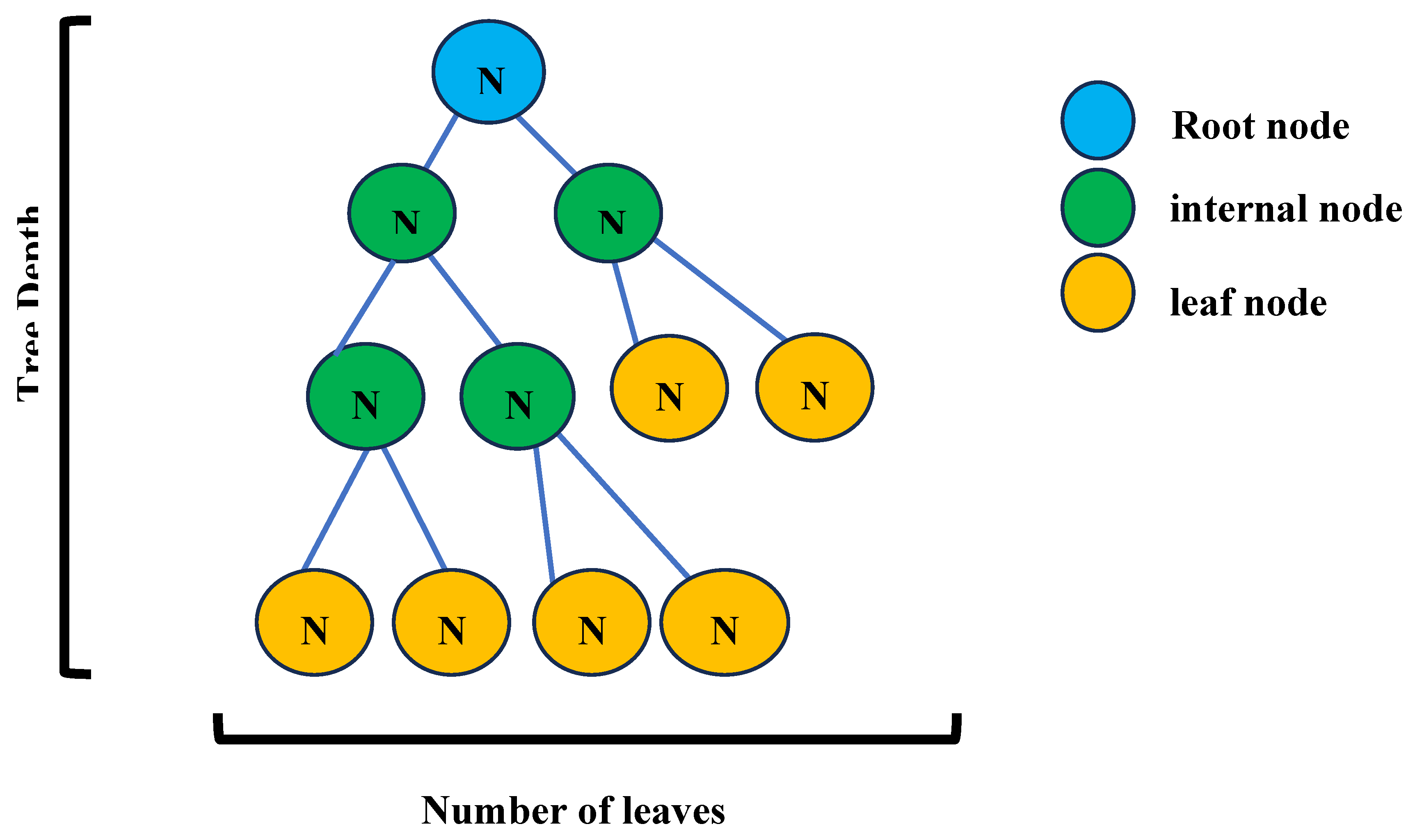
Figure 2.
Project workflow of the steps taken to develop the model and the varying complexities added across.
Figure 2.
Project workflow of the steps taken to develop the model and the varying complexities added across.
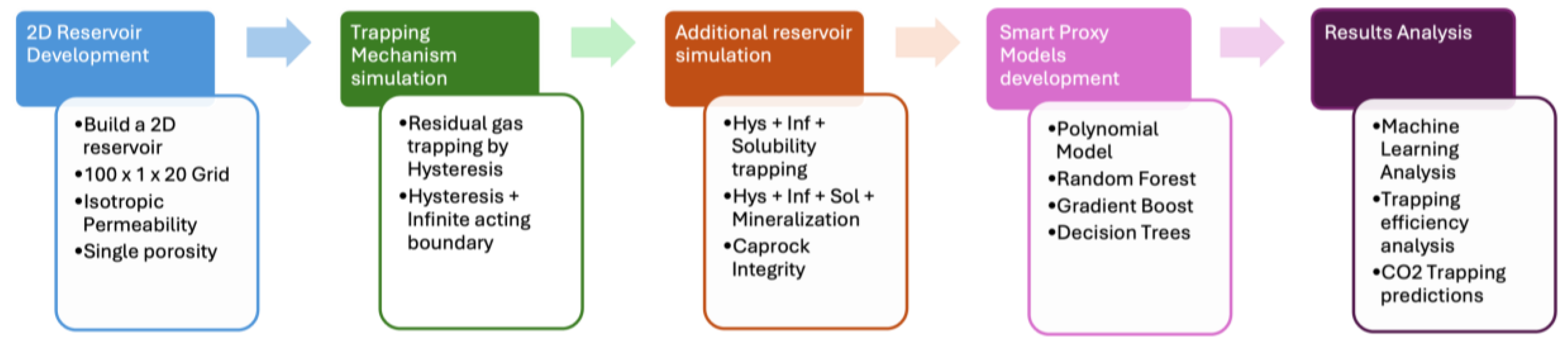
Figure 3.
Showing the IK-2D X-Sec profile of the grid in terms of Depth and Grid top.

Figure 4.
Hysteresis modelling for a water-gas system showing the drainage and imbibition curves[24].
Figure 4.
Hysteresis modelling for a water-gas system showing the drainage and imbibition curves[24].
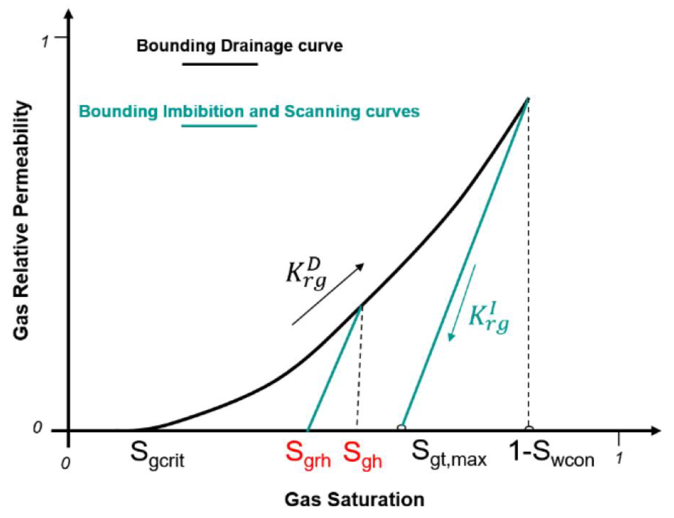
Figure 5.
The color legend on the right provides a scale representing the volume within different regions of the simulated reservoir model. The red region at the bottom of the grid corresponds to the simulated infinite-acting aquifer, which has been assigned a significantly increased volume compared to other areas in the model.
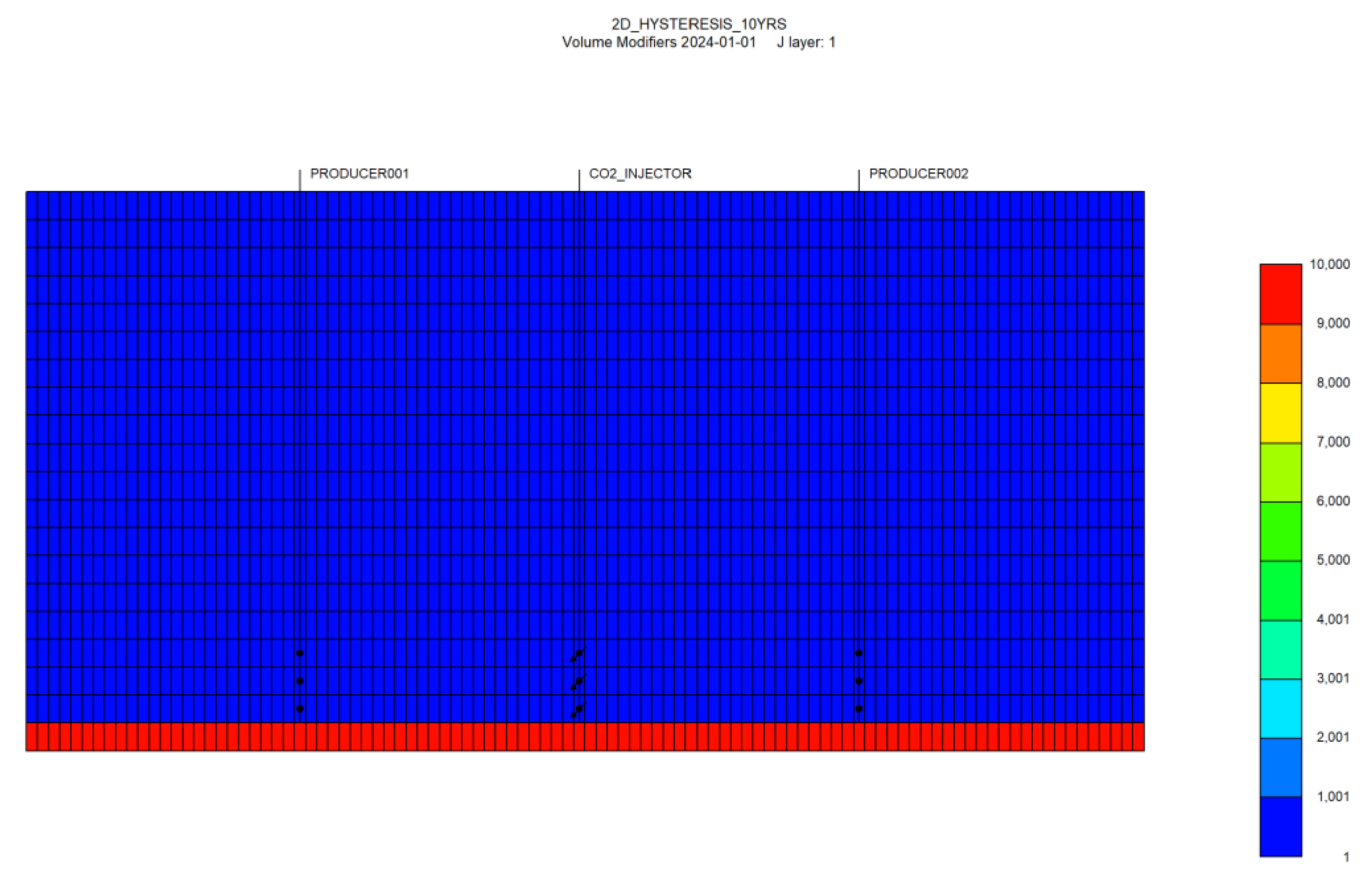
Figure 6.
Schematic demonstration of Pressure behavior with respect to depth [31].
Figure 6.
Schematic demonstration of Pressure behavior with respect to depth [31].
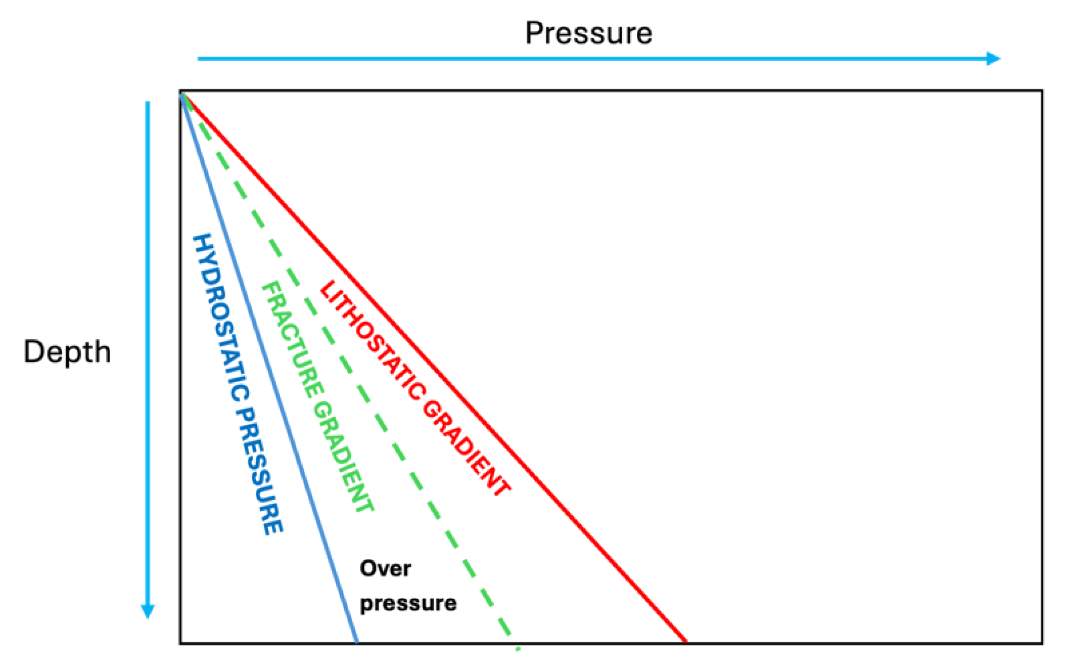
Figure 7.
Cross-sectional view of the reservoir model with the producer wells present while illustrating permeability distribution across layers. The blue section represents a layer of extremely low permeability, modeled to imply the presence of a caprock seal, which acts as a barrier to upward CO₂ migration.
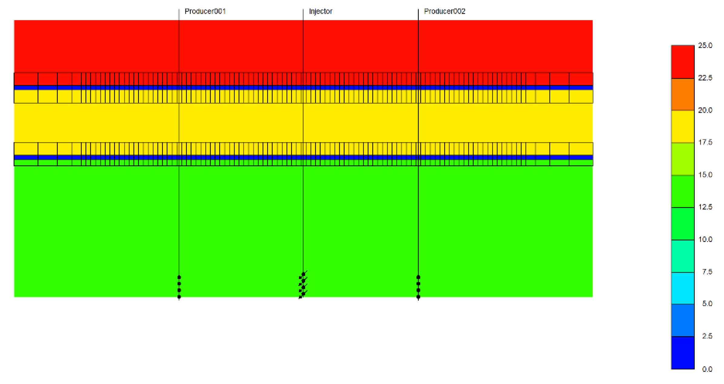
Figure 8.
Cross sectional permeability profile of the layers in the grid with just the injector well and no producers present.
Figure 8.
Cross sectional permeability profile of the layers in the grid with just the injector well and no producers present.
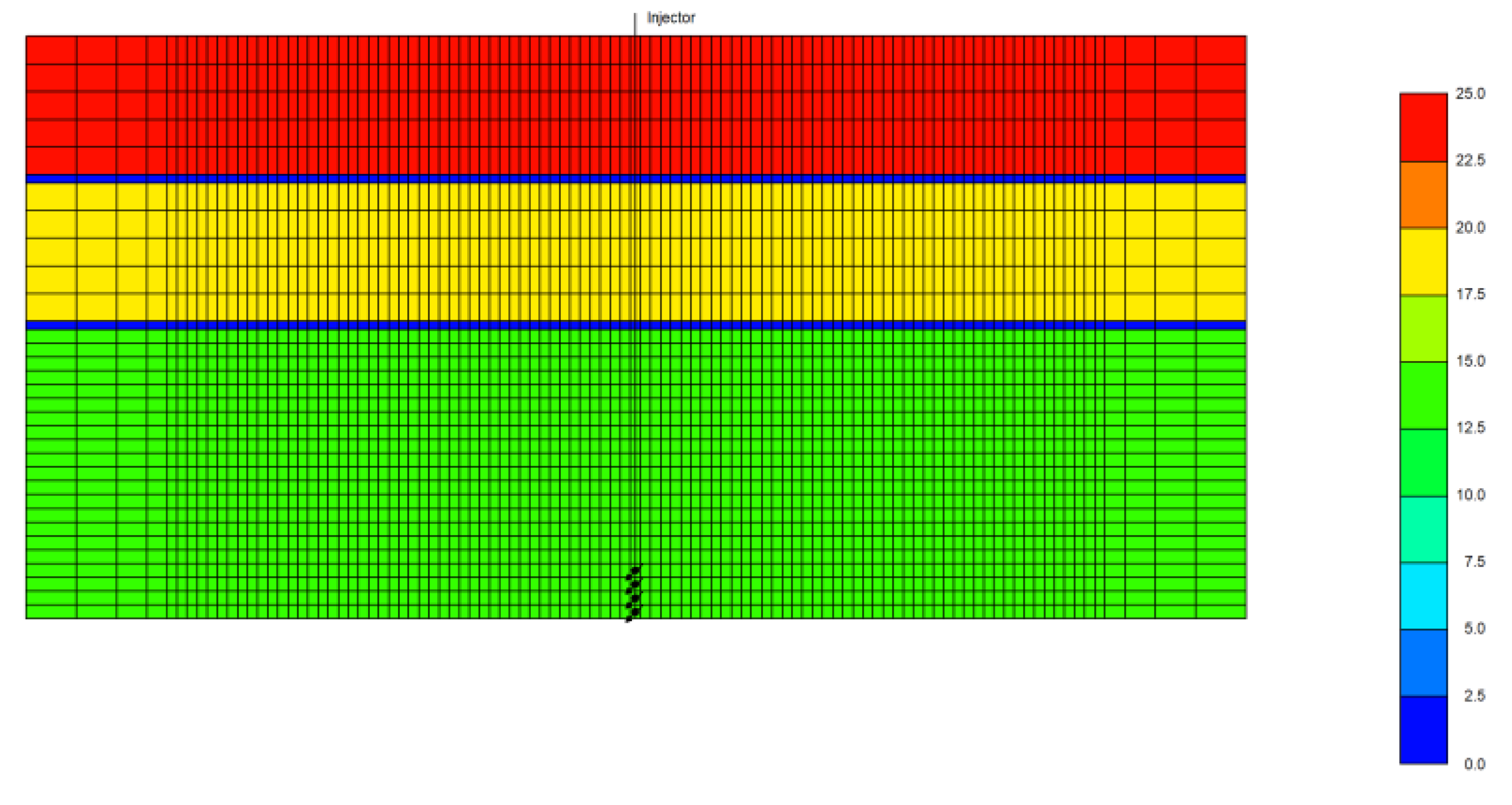
Figure 9.
This graph illustrates the dynamics of CO₂ trapped in different scenarios after the injection period ends in 2034. The trapping mechanisms, including hysteresis, solubility, mineralization, and their combinations, reveal distinct trends in storage performance over the monitoring period (2034–2074).
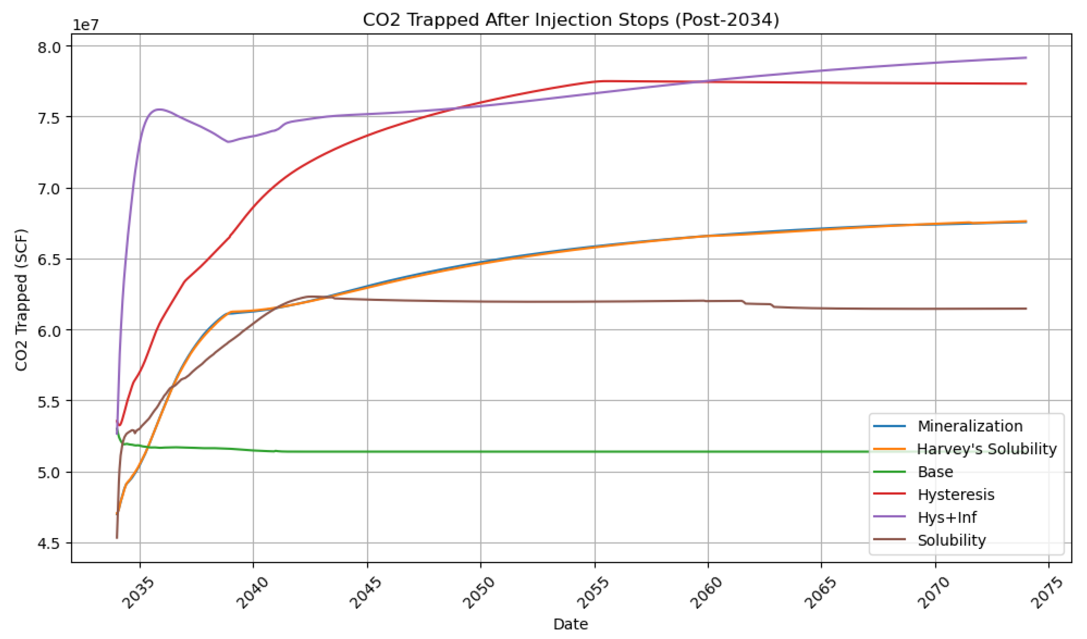
Figure 10.
(a): This bar chart compares the cumulative amount of CO₂ trapped by various mechanisms, excluding caprock effects, over the simulation period. Each trapping mechanism is evaluated based on its efficiency in immobilizing CO₂, revealing significant differences in storage performance; (b) Comparison of cumulative CO₂ trapped by different techniques: Caprock demonstrates unparalleled trapping efficiency (1.2 × 10⁹ SCF), emphasizing the critical role of structural trapping as the dominant mechanism for secure CO₂ containment.
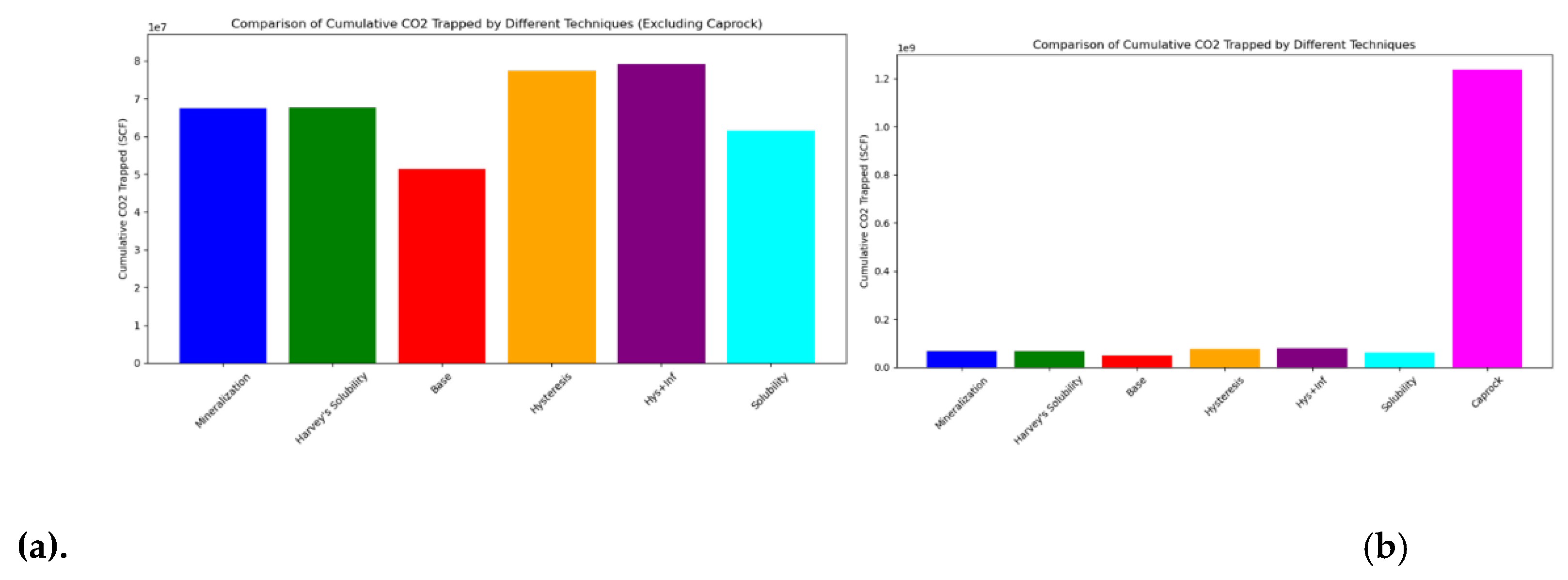

Table 1.
showing the reservoir properties parameters used in developing the base case model for simulation.
Table 1.
showing the reservoir properties parameters used in developing the base case model for simulation.
| Parameter | Value |
|---|---|
| Grid top (m) | 1200 |
| Grid thickness(m) Grid dimension Porosity(%) Permeability I direction (md) Permeability j direction(md) Permeability k direction(md) Compressibility, 1/kPa Pressure, kPa Temperature, oC Block width, m CO2 Injector well address Producer 1 well address Producer 2 well address Injection rate m3/day |
5 100 x 1 x 20 0.18 100 100 100 5.8e-7 11800 50 10 10 1 17:19 25 1 17:19 75 1 17:19 1,000,000 |
Table 2.
Constraints of the wells.
| Well type | Constraint | Parameter | Limit/Mode | Value |
|---|---|---|---|---|
| CO2 Injector | OPERATE | STG surface rate | MAX | 1 x 10⁶ m3/day |
| CO2 Injector | OPERATE | BHP Bottomhole Pressure | MAX | 44500 kPa |
| Producer 1 | OPERATE | BHP Bottomhole Pressure | MIN | 10000 kPa |
| Producer 2 | OPERATE | BHP Bottomhole Pressure | MIN | 10000 kPa |
Table 3.
Parameters used in activating the Barton- Bandis Model.
| Parameter | Value |
|---|---|
| Initial fracture aperture | 1.981e-5 m |
| Initial normal fracture stiffness | 6.786e7 kPa/m |
| Fracture opening stress | 2000 kPa |
| Hydraulic fracture permeability | 233 md |
| Fracture closure permeability | 233 md |
| Residual value of fracture closure permeability | 233 md |
Table 4.
SPM performance across board, indicating predictive accuracy.
| Trapping Scenario | Model | Train R2 | Test R2 |
|---|---|---|---|
| Base Case | Decision Tree | 0.9691 | 0.9731 |
| Base Case | Gradient Boosting | 0.9954 | 0.9961 |
| Base Case | Random Forest | 0.9630 | 0.9714 |
| Hysteresis | Decision Tree | 0.9688 | 0.9710 |
| Hysteresis | Gradient Boosting | 0.9985 | 0.9991 |
| Hysteresis | Random Forest | 0.9627 | 0.9714 |
| Hysteresis+Infinite Aquifer | Decision Tree | 0.9691 | 0.9731 |
| Hysteresis+Infinite Aquifer | Gradient Boosting | 1.0000 | 0.9987 |
| Hysteresis+Infinite Aquifer | Random Forest | 0.9627 | 0.9739 |
| Solubility | Decision Tree | 0.9697 | 0.9665 |
| Solubility | Gradient Boosting | 0.9959 | 0.9954 |
| Solubility | Random Forest | 0.9630 | 0.9739 |
| Mineralization | Decision Tree | 0.9697 | 0.9664 |
| Mineralization | Gradient Boosting | 0.9979 | 0.9975 |
| Mineralization | Random Forest | 0.9470 | 0.9392 |
Disclaimer/Publisher’s Note: The statements, opinions and data contained in all publications are solely those of the individual author(s) and contributor(s) and not of MDPI and/or the editor(s). MDPI and/or the editor(s) disclaim responsibility for any injury to people or property resulting from any ideas, methods, instructions or products referred to in the content. |
© 2025 by the authors. Licensee MDPI, Basel, Switzerland. This article is an open access article distributed under the terms and conditions of the Creative Commons Attribution (CC BY) license (http://creativecommons.org/licenses/by/4.0/).
Copyright: This open access article is published under a Creative Commons CC BY 4.0 license, which permit the free download, distribution, and reuse, provided that the author and preprint are cited in any reuse.


