

Submitted:
24 June 2025
Posted:
26 June 2025
You are already at the latest version
Abstract
This technical note proposes a new index, the “distribution non-uniformity index (DNUI)”, for quantitatively measuring the non-uniformity or unevenness of a probability distribution relative to a baseline uniform distribution. The proposed DNUI is a standardized, distance-based metric ranging between 0 and 1, with 0 indicating perfect uniformity and 1 indicating extreme non-uniformity. It is applicable to both discrete and continuous probability distributions. Several examples are presented to demonstrate its application and to compare it with two classical evenness measures: Simpson’s evenness and Buzas & Gibson’s evenness.
Keywords:
probability distribution
; non‐uniformity
; unevenness
; uniformity
1. Introduction
Non-uniformity, or unevenness, is an inherent characteristic of probability distributions, as outcomes or values from a probability system are typically not distributed uniformly or evenly. Although the shape of a distribution can offer an intuitive sense of its non-uniformity, researchers often require a quantitative measure to assess this property. Such a measure is valuable for constructing distribution models and for comparing the non-uniformity across different distributions in a consistent and interpretable way.
A probability distribution is considered uniform when all outcomes have equal probability in the discrete case, or when the probability density is constant in the continuous case. Therefore, the uniform distribution serves as the natural baseline for assessing the non-uniformity of any given distribution, and non-uniformity is referred to as the degree to which a distribution deviates from this uniform benchmark. It is essential to ensure that the distribution being evaluated and the baseline uniform distribution share the same support. This requirement is especially important in the continuous case, where a fixed and clearly defined support is crucial for meaningful comparison.
The Kullback–Leibler (KL) divergence can be employed as a metric for measuring the non-uniformity of a given distribution by quantifying how different the distribution is from a baseline uniform distribution. A small KL divergence value indicates that the distribution is close to uniform. The KL divergence is applicable in both the discrete case and in the continuous case provided that the support is fixed. However, one significant drawback of using the KL divergence in this context is that it is unbounded. While a KL divergence value of zero represents perfect uniformity, there is no natural upper limit that allows us to contextualize how “non-uniform” a distribution is. This lack of an upper bound can make interpretation challenging, especially when comparing different distributions or when the scale of the divergence matters.
In recent work, Rajaram et al. (2024a, b), proposed a measure called the “degree of inequality (DOI)” to quantify how evenly the probability mass or density is distributed across available outcomes or support. Specifically, they defined the DOI for a partial distribution on a fixed interval as the ratio of the exponential of the Shannon entropy to the coverage probability of that interval (Rajaram et al., 2024a, b)
where the subscript “P” denotes “part”, referring to the partial distribution on the fixed interval, is the coverage probability of the interval, is the entropy of the partial distribution, and is the entropy-based diversity of the partial distribution. When the entire distribution is considered, , and thus, the DOI equals the entropy-based diversity . It should be noted that the DOI is neither standardized nor normalized and does not explicitly measure the deviation of the given distribution relative to a uniform benchmark.
Classical evenness measures, such as Simpson’s evenness and Buzas & Gibson’s evenness, are essentially diversity ratios. For a discrete random variable X with probability mass function (PMF) and n possible outcomes, Simpson’s evenness is defined as (e.g., Roy & Bhattacharya, 2024)
where is Simpson’s diversity, representing the effective number of distinct elements in the probability system , and n is the maximum diversity that corresponds to a uniform distribution with PMF 1/n. The concept of effective number is the core of diversity measures in biology (Jost, 2006).
Buzas & Gibson’s evenness is defined as (Buzas & Gibson, 1969)
where is the Shannon entropy of X, , and is the extropy of the uniform distribution with PMF 1/n. The exponential of the Shannon entropy is the entropy-based diversity, and it also considered to be an effective number of elements in the probability system .
Unlike the DOI, which is not normalized, both and are normalized by n, the maximum diversity corresponding to the baseline uniform distribution. Therefore, these indices range between 0 and 1, with 0 indicating extreme unevenness and 1 indicating perfect evenness.
However, as Gregorius and Gillet (2021) pointed out, “Diversity-based methods of assessing evenness cannot provide information on unevenness, since measures of diversity generally do not produce characteristic values that are associated with states of complete unevenness.” This limitation arises because diversity measures are primarily designed to capture internal distribution characteristics, such as concentration and relative abundance within the distribution. For example, the quantity is often called “repeat rate” or Simpson index (Rousseau, 2018), or Simpson concentration (Jost, 2006); it has historically been used as a measure of concentration (Rousseau, 2018). Moreover, since diversity metrics are not constructed within a comparative distance framework, they inherently lack the ability to quantify deviations from uniformity in a meaningful or interpretable way. This limitation significantly diminishes their effectiveness when the goal is specifically to detect or describe high degrees of non-uniformity.
It is important to emphasize that the non-uniformity or unevenness of a distribution should be quantified by explicitly measuring its distance from the ideal of perfect uniformity. However, neither the DOI nor the evenness indices and calculate an explicit distance relative to a uniform benchmark.
The aim of this study is to develop a new standardized, distance-based index that can effectively quantify the non-uniformity or unevenness of a probability distribution. In the following sections, Section 2 describes the proposed distribution non-uniformity index (DNUI). Section 3 presents several examples. Section 4 provides discussion and conclusion.
2. The Proposed Distribution Non-Uniformity Index (DNUI)
The mathematical formulation of the proposed distribution non-uniformity index (DNUI) differs for discrete and continuous random variables.
2.1. Discrete Cases
Consider a discrete random variable X with probability mass function (PMF) and n possible outcomes. Let denote the uniform distribution with the same possible outcomes, so that for all x. We use this uniform distribution as the baseline for measuring the non-uniformity of the distribution of X.
The difference between the two PDFs and is given by
Thus,can be written as
Taking squares on both sides of Eq. (5) yields
Then, taking the expectation on both sides of Eq. (6) yields
whereis called the total variance andis called the total deviation
where is the variance of relative to , given by
is the bias of relative to , given by
where is called the (discrete) informity of X in the theory of informity proposed by Huang (2025), which is the expectation of the PMF. The informity of the baseline uniform distribution is .
Definition 1.
The proposed DNUI (denoted by
) for the distribution of X is given by
where is the root mean square (RMS) of and is the second moment of the probability , given by
2.2. Continuous Cases
Consider a continuous random variable Y with probability density function (PDF) defined on an unbounded support, such as ). Since there is no baseline uniform distribution defined over an unbounded support, we cannot measure the non-uniformity of the entire distribution. Instead, we examine parts of the distribution on a fixed interval , which allows us to assess local non-uniformity.
According to Rajaram et al. (2024a), the PDF of a partial distribution on is given by renormalization of the original PDF
where , which is the coverage probability of the interval .
Let denote the uniform distribution on with PDF . We use this uniform distribution as the baseline for measuring the non-uniformity of the partial distribution.
Similar to the discrete case, the difference between the two PDFs and is given by
Thus,can be written as
Taking squares on both sides of Eq. (15) yields
Then, taking the expectation on both sides of Eq. (16) yields
The total deviation is given by
where is the variance of relative to on , given by
and is the bias of relative to , given by
Definition 2. The proposed DNUI for the partial distribution on (denoted by ) is given by
where is the second moment of the PDF , given by
Definition 3. If the continuous distribution is defined on the fixed support , and, the proposed DNUI for the entire distribution of Y (denoted by ) is given by
where is the second moment of the PDF , given by
the variance is given by
and the bias is given by
The quantity is denoted by and is called the continuous informity of Y in the theory of informity (Huang, 2025).
3. Examples
3.1. Coin-Tossing
Consider tossing a coin, which is a simplest two-state probability system: {X; P(x)}={head, tail; P(head), P(tail)}, where . The DNUI for the distribution of X is given by
where the second moment can be calculated as
Figure 1 shows the DNUI for the distribution of X as a function of the bias represented by . The two evenness measures: Simpson’s evenness and Buzas & Gibson’s evenness are also shown in Figure 1 for comparison.
As shown in Figure 1, when the coin is fair (i.e. ), the DNUI is 0, and both Simpson’s evenness and Buzas & Gibson’s evenness equal 1, indicating perfect uniformity or evenness. As the coin becomes increasingly biased toward either head or tail, the DNUI increases, while and decrease. In the extreme case where or , the DNUI reaches its maximum value of , reflecting a high degree of non-uniformity. However, in this case, both and reach their minimum value of 0.5, which fails to capture the true extent of unevenness. This supports the argument made by Gregorius and Gillet (2021): “… measures of diversity generally do not produce characteristic values that are associated with states of complete unevenness.”
3.2. Three Frequency Data Series
JJC (2024) posted a question on Cross Validated about quantifying distribution non-uniformity. He supplied three frequency datasets (Series A, B, and C), each containing 10 values (Table 1). Visually, Series A is almost perfectly uniform, Series B is nearly uniform, and Series C is heavily skewed by a single outlier (0.6). Table 1 lists these datasets alongside the corresponding DNUI, , and values.
From Table 1, we can see that the DNUI value for Series A is 0.1864, confirming its high uniformity, while the DNUI value for Series B is 0.2499, indicating near-uniformity. In contrast, the DNUI value for Series C is 0.9767 (close to 1), signaling extreme non-uniformity. These results align well with intuitive expectations. The and values for Series A and Series B are both close to 1, also indicating high uniformity. The value for Series C is 0.2625, capturing its pronounced unevenness. However, the value for Series C remains relatively high at 0.4545, failing to adequately reflect the severity of non-uniformity.
3.3. Five Continuous Distributions with Fixed Support
Consider five continuous distributions with fixed support : uniform, triangular, quadratic, raised cosine, and half-cosine. Table 2 summarizes their PDFs, variances, biases, second moments, and DNUIs.
As shown in Table 2, the DNUI is independent of the scale parameter a, which is a desirable property for a measure of distribution non-uniformity. By definition, the DNUI for the uniform distribution is 0. In contrast, the DNUI values for the other four distribution range from 0.5932 to 0.7746, indicating moderate to high non-uniformity. These results align well with intuitive expectations. Notably, the raised cosine distribution has the highest DNUI value among the five distributions, suggesting it exhibits the greatest non-uniformity.
3.4. Exponential Distribution
The PDF of the exponential distribution with support is
where is the shape parameter.
We consider a partial exponential distribution on the interval [ (i.e., and ), where b is the length of the interval. Thus, the DNUI for the partial exponential distribution is given by
where the second moment is given by
The coverage probability of the interval [ is given by
The integral can be solved as
Figure 2 shows the plot of the DNUI for the partial exponential distribution with as a function of the interval length b. It also shows the PDF of the original exponential distribution, Eq. (29) with , as a function of y.
As shown in Figure 2, when the interval length b is very small (approaching 0), the DNUI is close to 0, reflecting the high local uniformity within small intervals. As the interval length b increases, the DNUI also increases, indicating the growing local non-uniformity with larger intervals. When the interval length b becomes very large, the DNUI approaches 1, indicating that the distribution over a large interval is extremely non-uniform. These observations align well with intuitive expectations.
4. Discussion and Conclusions
Unlike the degree of inequality (DOI) or the existing evenness measures such as and (which are not distance measures), the proposed distribution non-uniformity index (DNUI) is a standardized, distance-based metric derived from the total deviation defined in Eq. (8). Importantly, this total deviation incorporates two components: variance and bias, both measured relative to the baseline uniform distribution. In contrast, the DOI, , and are not distance-based metrics and therefore cannot effectively quantify unevenness. As noted by Gregorius and Gillet (2021), diversity-based evenness measures do not capture deviations from uniformity in a meaningful way and fail to provide characteristic values that represent complete unevenness.
The proposed DNUI ranges between 0 and 1, with 0 indicating perfect uniformity and 1 indicating extreme non-uniformity. Lower DNUI values (close to 0) suggest a more uniform or flatter distribution, while higher values (close to 1) suggest a greater degree of non-uniformity or unevenness. Although there are no universally accepted benchmarks for defining levels of non-uniformity, we tentatively propose DNUI values of 0.25, 0.5, and 0.75 to represent low, moderate, and high non-uniformity, respectively, based on the examples presented in this study.
It is important to note that the DNUI depends solely on the probability values and not on the associated outcomes (or scores) or their specific order. This property can be illustrated using the frequency data from Series C in Subsection 3.1: {0.03, 0.02, 0.6, 0.02, 0.03, 0.07, 0.06, 0.05, 0.05, 0.07}. If, for example, the second and third values are swapped, the DNUI value remains unchanged. This invariance implies that different distributions can yield the same DNUI value. In other words, the DNUI is not a one-to-one function of the distribution; it can “collapse” different distributions into the same value. This property is analogous to how different distributions can share the same mean or variance.
In summary, the proposed DNUI provides an effective metric for quantifying the non-uniformity or unevenness of probability distributions. It is applicable to any distributions, discrete or continuous, defined on a fixed support. It can also be applied to partial distributions on fixed intervals to examine local non-uniformity, even when the overall distribution has unbounded support. The presented examples have demonstrated the effectiveness of the proposed DNUI in capturing and quantifying distribution non-uniformity.
References
- Buzas MA, Gibson TG. (1969). Species diversity: benthonic foraminifera in western North Atlantic. Science, 163(3862), 72-5.
- Gregorius, H. R., & Gillet, E. M. (2021). The Concept of Evenness/Unevenness: Less Evenness or More Unevenness? Acta biotheoretica, 70(1), 3. [CrossRef]
- Huang, H. (2025). The theory of informity: a novel probability framework. To be published in Bulletin of Taras Shevchenko National University of Kyiv.
- JJC (https://stats.stackexchange.com/users/10358/jjc), How does one measure the non-uniformity of a distribution? URL (version: 2024-10-12): https://stats.stackexchange. 2582.
- Jost, L. (2006). Entropy and diversity. Oikos, 113, 363–375.
- Rajaram, R., Ritchey, N., & Castellani, B. (2024a). On the mathematical quantification of inequality in probability distributions. Journal of Physics Communications,8(8), Article 085002. [CrossRef]
- Rajaram, R., Ritchey, N., & Castellani, B. (2024b). On the degree of uniformity measure for probability distributions. J. Phys. Commun. 8 115003.
- Rousseau, R. (2018). The repeat rate: from Hirschman to Stirling. Scientometrics, 116, 645–65. [CrossRef]
- Roy, S., & Bhattacharya, K. R. (2024). A theoretical study to introduce an index of biodiversity and its corresponding index of evenness based on mean deviation. World Journal of Advanced Research and Reviews, 21(2), 022-032. [CrossRef]
Figure 1.
The DNUI for the distribution of X as a function of the bias represented by the probability of heads, compared with Simpson’s evenness and Buzas & Gibson’s evenness
Figure 1.
The DNUI for the distribution of X as a function of the bias represented by the probability of heads, compared with Simpson’s evenness and Buzas & Gibson’s evenness
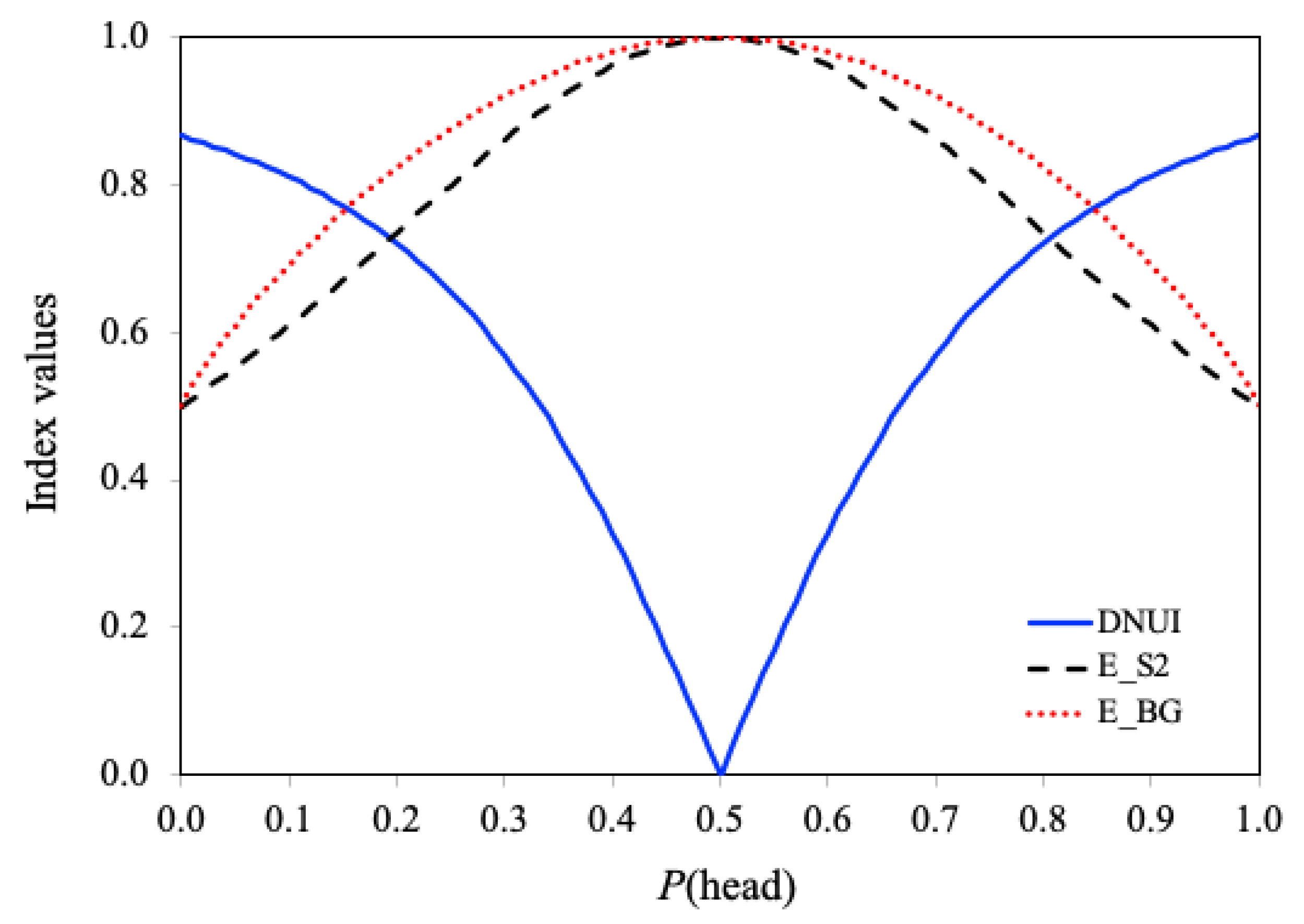
Figure 2.
Plots of the DNUI for the partial exponential distribution with and the PDF of the original exponential distribution.
Figure 2.
Plots of the DNUI for the partial exponential distribution with and the PDF of the original exponential distribution.
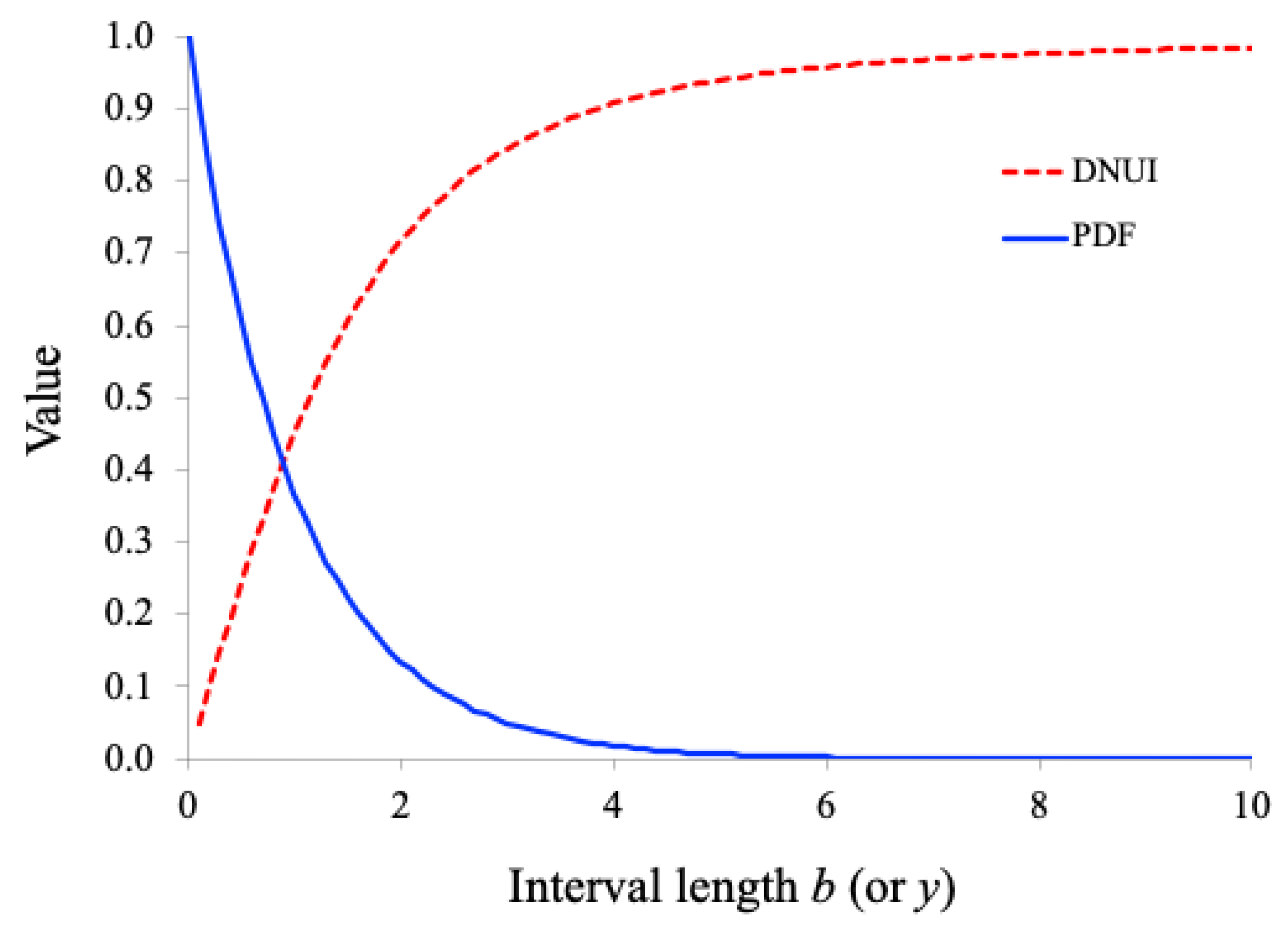

Table 1.
Three frequency data series and the corresponding DNUI, , and values.
| Series |
|
|
|
|---|---|---|---|
| A: {0.1, 0.11, 0.1, 0.09, 0.09, 0.11, 0.1, 0.1, 0.12, 0.08} | 0.1864 | 0.9881 | 0.9940 |
| B: {0.1, 0.1, 0.1, 0.08, 0.12, 0.12, 0.09, 0.09, 0.12, 0.08} | 0.2499 | 0.9785 | 0.9891 |
| C: {0.03, 0.02, 0.6, 0.02, 0.03, 0.07, 0.06, 0.05, 0.05, 0.07} | 0.9767 | 0.2625 | 0.4545 |
Table 2.
The PDF , variance , bias , second moment , and DNUI for five continuous distributions with fixed support
Table 2.
The PDF , variance , bias , second moment , and DNUI for five continuous distributions with fixed support
| Distribution |
|
|
|
|
|
| Uniform |
|
0 | 0 |
|
0 |
| Triangular |
|
|
|
|
0.7071 |
| Quadratic |
|
|
|
|
0.5932 |
| Raised cosine |
|
|
|
|
0.7746 |
| Half-cosine |
|
|
|
|
0.6262 |
Disclaimer/Publisher’s Note: The statements, opinions and data contained in all publications are solely those of the individual author(s) and contributor(s) and not of MDPI and/or the editor(s). MDPI and/or the editor(s) disclaim responsibility for any injury to people or property resulting from any ideas, methods, instructions or products referred to in the content. |
© 2025 by the authors. Licensee MDPI, Basel, Switzerland. This article is an open access article distributed under the terms and conditions of the Creative Commons Attribution (CC BY) license (http://creativecommons.org/licenses/by/4.0/).
Copyright: This open access article is published under a Creative Commons CC BY 4.0 license, which permit the free download, distribution, and reuse, provided that the author and preprint are cited in any reuse.


