
Submitted:
30 April 2025
Posted:
02 May 2025
You are already at the latest version
Abstract
Maxwell’s electromagnetic wave theory has provided the foundation for life- changing and life-saving technologies from smartphones to magnetic resonance imaging. This is especially intriguing given that Maxwell’s electromagnetic wave is inconsistent with the fundamental scientific principles of causality and conservation of energy, as well as the assumption of the Kirchhoff diffraction integral, which is the fundamental equation used in optics to relate the object to the image. These contradictions exist because Maxwell arbitrarily considered the waves that represent the magnetic and electric fields to be in-phase. In this article, I show that the reintroduction of the “evil” magnetic vector potential resolves the contradictions by giving a first principle approach to the claim that the waves that represent the magnetic and electric fields are a quadrature out-of-phase.
Keywords:
magnetic vector potential
; Maxwell’s equations
; electromagnetic wave
; causality
; conservation of energy
; Kirchhoff’s diffraction equation
; binary photon
1. Introduction
James Clerk Maxwell [1] is one of the most brilliant and influential scientists who ever lived. By combining the equations that describe Gauss’, Faraday’s, and Ampere’s laws of electricity and magnetism, he was able to unify electricity, magnetism, and optics and predict that light propagates as an electromagnetic wave though a vacuum at a speed characterized by the electric permittivity and the magnetic permeability of the vacuum [2], and it propagates through a dielectric at a slower speed characterized by the relative permittivity and relative permeability of the dielectric [3].
Einstein [4] described Maxwell’s discovery like so:
Imagine his feelings when the differential equations he had formulated proved to him that electromagnetic fields spread in the form of polarized waves, and at the speed of light! To few men in the world has such an experience been vouchsafed. At that thrilling moment he surely never guessed that the riddling nature of light, apparently so completely solved, would continue to baffle succeeding generations. Meantime, it took physicists some decades to grasp the full significance of Maxwell’s discovery, so bold was the leap that his genius forced upon the conceptions of his fellow-workers.
Maxwell’s electromagnetic wave theory, was based on Faraday’s [5] idea that radiation was “a high species of vibration in the lines of force which are known to connect particles and also masses of matter together.” However, Maxwell’s electromagnetic wave equation neglected the particles that served as the sources and sinks of the electromagnetic vibrations, and which are now known as electrons. Few [6] worried about the omission after the marvelous experimental researches of Heinrich Hertz [7] demonstrated the reality of electromagnetic radio waves propagating through free space using a linear antenna to detect the electric field and a hoop antenna to detect the magnetic field. The successful application of electromagnetic waves in technologies, including smartphones, television, radio, radar, microwave ovens, microscopes, CAT scans, and MRI, provided no impetus for questioning Maxwell’s electromagnetic wave equation.
Maxwell’s equations for free space are typically given in vector form in terms of the electric field (E, in ) and the magnetic field (B, in ) that exist between the unaccounted-for sources and sinks.
where is the charge density (in ), is the magnetic permeability of the vacuum (in ), is the electric permittivity of the vacuum (in ), and is the current density (in ), which is set to zero for free space. By also letting , Maxwell obtained the homogeneous second-order differential electromagnetic wave equations for the E field and B field:
There is nothing in the above equations that stipulate the phase relationship between the electric and magnetic fields. Nevertheless, Maxwell [8] considered the two fields to be in-phase (Figure 1) rather than having one precede the other; and to this day, the E and B fields are typically considered to be in-phase [9,10]. It was as if Maxwell had not removed the possibility of instantaneous action-at-a-distance from his field theory.
It seems to me that too much fundamental science must be sacrificed to continue to represent the electric and magnetic fields in-phase.
- We sacrifice the cause-and-effect relationship inferred in Faraday’s and Ampere’s laws if the waves representing the electric and magnetic fields are in-phase.
- We sacrifice the conviction that the conversion of one form of energy into another form cannot take place instantaneously as demanded by special relativity. Having the electric and magnetic fields in-phase implies instantaneous action-at-a-distance.
- We sacrifice conservation of energy in the electromagnetic field if the waves representing the amplitudes of the electric and magnetic fields are in-phase, since at successive points in time, the energy in the electromagnetic field, which is proportional to the square of the amplitudes, will go from zero to maximum and back to zero [11].
- We also sacrifice the demand of Kirchhoff’s diffraction equation, based on Green’s theorem, that both the Neumann and the Dirichlet boundary conditions be simultaneously fulfilled at a boundary [12].
While Maxwell’s wave equation has been extremely successful in serving as a foundation for technological development, Maxwell’s electromagnetic wave theory leaves something to be desired when it comes to creating a consistent and logically-uniform set of laws that coherently explain natural phenomena. After all, Einstein [4] describes “science” as “the attempt to make chaotic diversity of our sense-experience correspond to a logically uniform system of thought.” The aim of this work is to take a second look at Maxwell’s electromagnetic wave theory in order to develop a logically uniform and consistent set of equations that coherently explain natural phenomena. To do so, I return to Faraday’s [6] conception of particles and fields and employ the magnetic vector potential to connect and unite the particles with the fields.
2. Results
Maxwell [13] considered that the magnetic vector potential represented “the fundamental quantity in the theory of electromagnetism,” yet by the end of the 19th century, the magnetic vector potential lost favor. Oliver Heaviside [14] considered the magnetic vector potential “evil” and “cured” Maxwell’s equations by writing the magnetic vector potential out of them. Generally, with only a few exceptions, Heaviside’s form of Maxwell’s equations is considered to be Maxwell’s equations, and except for a few holdouts [15,16,17], the magnetic vector potential has been considered merely a mathematical device used to help in calculations but not something that had physical meaning or something that was based in reality [18,19]. Here I will show that the generation of electromagnetic radiation by moving electrons in an antenna (Figure 2) is best understood using the magnetic vector potential. Then I will show that the electromagnetic waves described by the curl of the magnetic vector potential are consistent with causality, conservation of energy, and the Kirchhoff diffraction equation.
The magnetic vector potential is defined for a static case like so:
where A (in ) is the magnetic vector potential produced by a current density (J, in ) at a source point () and measured at a field point (r) where r and are position vectors in a Cartesian coordinate system starting at the origin (0,0,0), and . The magnetic vector potential is integrated over an infinitesimal volume that includes the source point. The magnetic vector potential vanishes at infinity. is the magnetic permeability of the vacuum and is equal to .
In magnetostatics, the static magnetic field () is related to the magnetic vector potential in the following manner:
When the current density is time-varying, the magnetic vector potential is time dependent, and to take into consideration the fact that it takes time for the magnetic vector potential to propagate from to r, the retarded time must be used to characterize the source when the field is measured at the present time (t). Assuming that the magnetic vector potential propagates a distance R from the source point to a point in the field at the speed of light (c), then the retarded time is given by:
and the time-dependent magnetic vector potential is given by:
This form of the equation establishes temporal causality between the source and the field and ensures that the magnetic vector potential propagates at the speed of light. While the static case of the magnetic vector potential implies instantaneous action-at-a-distance, the time-dependent case that includes the retarded time is based firmly on causality where the magnetic vector potential propagates from source point to the field point at the speed of light. Equation 6 bridges potential theory with field theory.
I propose that the electric and magnetic fields produced by the curl of the time-varying current density () can be calculated from the curl of the magnetic vector potential . I will show that when taking the curl of the time-dependent magnetic vector potential, the two complementary fields emerge. The magnetic field emerges directly as it does when taking the curl of the static magnetic vector potential; however, in the time-dependent case, the electric field also emerges after multiplying the semi-integral by the speed of light.
Taking the curl of both sides of Equation 6, we get:
To simplify Equation 6, we use the vector identity:
where and . Thus
We solve for the first term in the integrand, using the definition of curl of in Cartesian coordinates:
hen resolve the curl into its three orthogonal components , , and , multiply each term by , let , , , , and rearrange to get:
Simplify by using the definition of curl in Cartesian coordinates, :
Then solve for the last term in the integrand.
Then insert Equation 13 into Equation 12:
After rearranging, we get:
Now, split the integral into two parts:
and define each part.
The first part is proportional to and inversely proportional to R. It represents the electric part (in Tesla or ):
The second part is proportional to J and inversely proportional to. It represents the magnetic part (in Tesla or ):
Tesla is the unifying unit of the electromagnetic field.
Equation 17 is directly equal to the magnetic field (, in Tesla or ):
To express the electric part as the electric field (), we must multiply the r.h.s. of Equation 17 by c:
Since is a constant, we can take it out of the integral and cancel:
and in Equations 19 and 21 describe the magnetic and electric fields produced by a dipole antenna. and in the denominators of Equations 19 and 21 represent a circular magnetic wave and a plane electric wave, respectively. The circular wave is consistent with and J. A linear wave requires acceleration where .
If we assume that the current density in a half-wavelength dipole antenna has the following form:
where is the angular frequency, then the magnetic field that results from the sinusoidally-varying current density will have the identical form. By contrast, the electric field that results from the sinusoidally-varying temporal derivative of the current density () will have this form:
Consequently, the magnetic and electric fields will be a quadrature out-of-phase with each other, and this satisfies causality, conservation of energy, and the boundary conditions demanded by Kirchhoff’s diffraction equation. The contradiction is resolved.
At a given position in the field, the sinusoidal waves described by Equations 24 and 25 are out-of-phase (Figure 3). They remain out-of-phase from the near-field through the far-field.
Since the magnetic and electric waves presented here are out-of-phase, the traditional equations that relate the square of the amplitude of the fields to the energy density are not applicable. Using Equations 24 and 25, the magnetic energy density (, in ) and the electrical energy density (, in ) at any point in space and time are given by:
Figure 3 illustrates the magnetic field as if it vibrated in a single plane like the electric field. According to Equation 24, it is actually a circular wave vibrating in a plane, which is consistent with the fact that there are no magnetic monopoles (Figure 4).
While the phase relationship between the and fields were obtained using the curl of the magnetic vector potential, we must return to Faraday’s law (Equation 1c) to justify the orthogonal relationship. The orthogonal relationship between and comes directly from the definition of the curl. Moreover, since , Faraday’s Law (Equation 1c) can be written
Plotting the electric field on the abscissa and the magnetic field on the ordinate, we get a phasor diagram that shows that there is a quarter-wave lag between the E field and the B field (Figure 5).
Heaviside [20] simplified Maxwell’s equations in a way that made them at the same time more useful and less explanatory. By replacing the temporal derivative in Maxwell’s equations with the form of Maxwell’s equations given below emphasizes the phase relationships between , , and , incorporates Faraday’s [5] idea that radiation was “a high species of vibration in the lines of force which are known to connect particles and also masses of matter together,” and makes the theory of the electromagnetic wave, based on the magnetic vector potential, consistent with causality, conservation of energy, and Kirchhoff’s diffraction theory.
This form of Maxwell’s equations, which includes the imaginary number i, is like that used by electrical engineers.
3. Discussion
Maxwell’s electromagnetic wave theory where the magnetic and electric fields are in-phase are inconsistent with causality, conservation of energy, and the demands of the Kirchhoff diffraction integral. By reintroducing the “evil” magnetic vector potential to describe the magnetic and electric fields that emanate from an antenna, I have resolved the contradictions by showing that magnetic and electric fields are a quadrature out-of-phase from where they are produced in the near-field to where they radiate in the far-field.
This means that there is no need to perform the technique/trick of a multipole expansion to convert the out-of-phase magnetic and electric waves in the reactive near-field through a complicated mixture of phases in the radiative near-field to in-phase magnetic and electric waves in the far-field in order to be consistent with Maxwell’s electromagnetic wave theory where the magnetic and electric fields are in phase [21].
Funding
This research received no external funding.
Conflicts of Interest
The author declares no conflicts of interest.
References
- Maxwell, J.C. A dynamical theory of the electromagnetic field. Philos. Trans. R. Soc. Lond. 1865, 155, 459–512. [Google Scholar]
- Maxwell. J.C. On a method of making a direct comparison of electrostatic with electromagnetic Force; with a note on the electromagnetic theory of light. Philos. Trans. R. Soc. Lond. 1868. 158, 643–657. [CrossRef]
- Wayne, R. Light and Video Microscopy. 3rd ed.; Elsevier, Amsterdam, The Netherlands. 2019. p. 76.
- Einstein, A. Considerations concerning the fundaments of theoretical physics. Science 1940, 91, 487–492. [Google Scholar] [CrossRef]
- Faraday, M. Thoughts on ray-vibrations. Phil. Mag. S.3. 1846, 28, 325–350. [Google Scholar]
- Einstein, A. On the present status of the radiation problem. In The Collected Papers of Albert Einstein, The Swiss Years: Writings, 1900–1909; Stachel, J., Cassidy, D.C., Renn, J., Schulmann, R. Eds.; Princeton University Press, Princeton, New Jersey, USA, 1989; Volume 2, pp. 357–375.
- Hertz, H. Electric Waves being Researches on the Propagation of Electric Action with Finite Velocity through Space; Dover Publications: New York, New York, USA 1952; 107-194.
- Maxwell, J.C. A Treatise on Electricity and Magnetism; Volume 2; Dover Publications: New York, New York, USA, 1954. p. 439.
- Griffiths, D. Introduction to Electrodynamics, 2nd ed.; Prentice Hall: Englewood Cliffs, NJ, USA 1989. p. 357.
- Jefimenko, O.D., Electricity and Magnetism; Appleton-Century-Crofts, New York, New York, USA 1966. p. 532.
- Wayne, R. A description of the electromagnetic fields of a binary photon. African Review of Physics 2018, 13, 128–141. [Google Scholar]
- Wayne, R. The Kirchhoff diffraction equation based on the electromagnetic properties of the binary photon. African Review of Physics 2019, 19, 30–48. [Google Scholar]
- Bork, A.M. Maxwell and the vector potential. Isis 1967, 58, 210–222. [Google Scholar] [CrossRef]
- Heaviside, O. New (duplex) method of treating the electromagnetic equations. The flux of energy. In Electrical Papers; The Copley Publishers, Boston, MA USA 1925, Volume 2, p. 173.
- Ehrenberg, W.; Siday, R.E. The refractive index in electron optics and the principles of dynamics, Proc. Phys. Soc. B. 1949, 62, 8–21. [Google Scholar] [CrossRef]
- Peat, F.D. Infinite Potential. The Life and Times of David Bohm; Addison-Wesley, Reading, MA, USA. 1997.
- Wayne, R. The relationship between the optomechanical Doppler force and the magnetic vector potential. African Review of Physics 2013, 8, 283–296. [Google Scholar]
- Gray, A. A Treatise on Magnetism and Electricity; Macmillan, London, England. 1898. p. 52.
- Larmor, J. Aether and Matter. Cambridge University Press, Cambridge, England. p. 112.
- Heaviside, O. Electromagnetic Theory; The Electrician, London, England. 1893. pp. vi-xii.
- Heald, M.A.; Marion, J.B. Classical Electromagnetic Radiation, 2nd ed.; Saunders College Publishing, Fort Worth, TX USA. 1995.
- Wayne, R. The binary photon: A heuristic proposal to address the enigmatic properties of light. African Review of Physics 2020, 15, 74–91. [Google Scholar]
- Wayne, R. Nature of light from the perspective of a biologist: What is a photon? In Handbook of Photosynthesis, 4th ed.; Pessarakli, M., Ed.; CRC Press, Boca Raton, FL, USA. 2024; pp. 24-74.
Figure 1.
Electromagnetic wave in free space where the electric field and the magnetic field are in-phase as given in A Treatise on Electricity and Magnetism by Maxwell [8].
Figure 1.
Electromagnetic wave in free space where the electric field and the magnetic field are in-phase as given in A Treatise on Electricity and Magnetism by Maxwell [8].
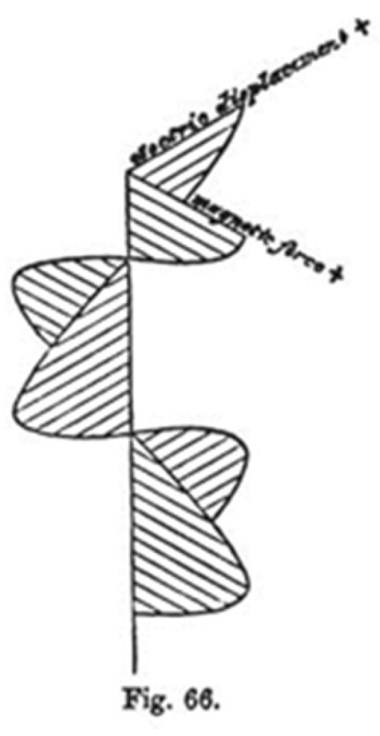
Figure 2.
Frame from an animation showing the A) maximal current (I(x)) in and the B) maximal voltage (V(x)) along a transmitting half-wavelength dipole antenna. The waves of current (green) and voltage (blue) reflect back and forth between the antennae ends to form standing waves where the I(x) wave is a quadrature out-of-phase with the V(x) wave. Source: Wikimedia commons https://commons.wikimedia.org/wiki/File:Dipole_antenna_standing_waves_animation_1-10fps.gif.
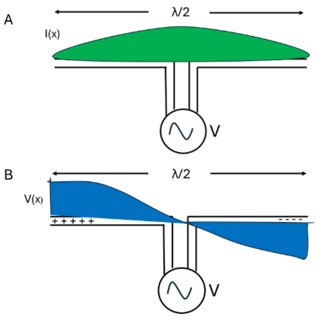
Figure 3.
A. An illustration of the magnetic (green) and electric (blue) fields at any point in free space according to the standard form of Maxwell’s equations. The magnetic and electric fields are in-phase. B. Using Equations 24 and 25 derived by using the magnetic vector potential, at any given point in free space, the magnetic (green) and electric (blue) fields are a quadrature out-of-phase.
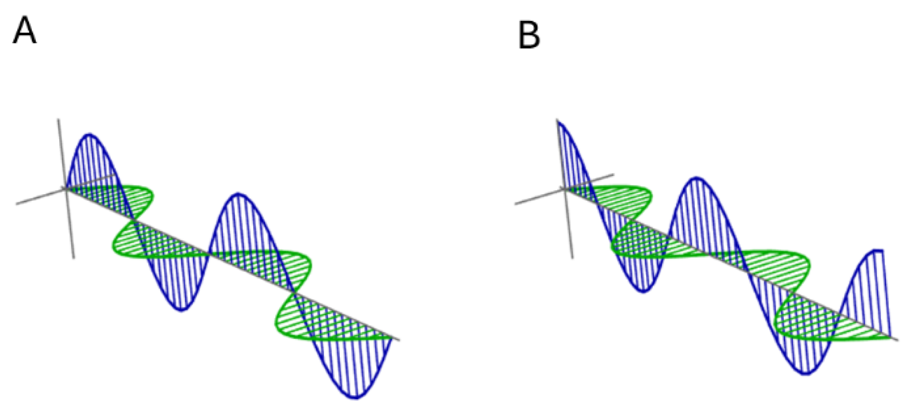
Figure 4.
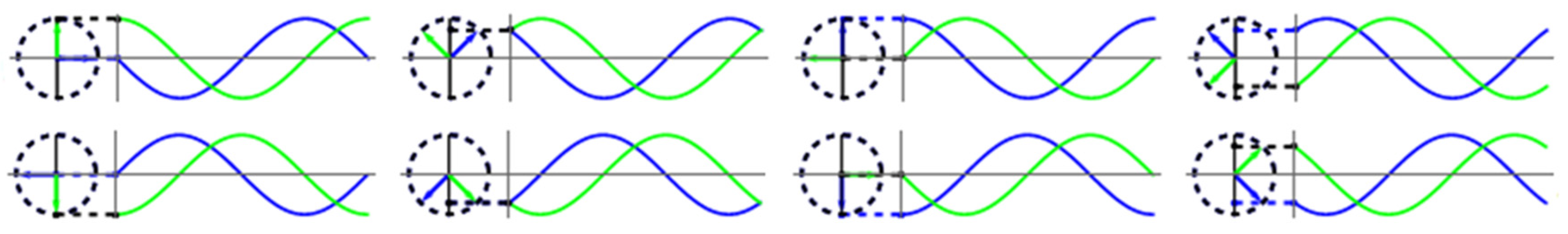
Images captured from an animation of the amplitudes of a circular magnetic wave (green circles) and a linear electric wave (blue arrow) propagating through free space. The amplitudes are a quadrature out-of-phase. The images were captured every 1/8 of a wavelength from a .gif.
Figure 4.
Images captured from an animation of the amplitudes of a circular magnetic wave (green circles) and a linear electric wave (blue arrow) propagating through free space. The amplitudes are a quadrature out-of-phase. The images were captured every 1/8 of a wavelength from a .gif.
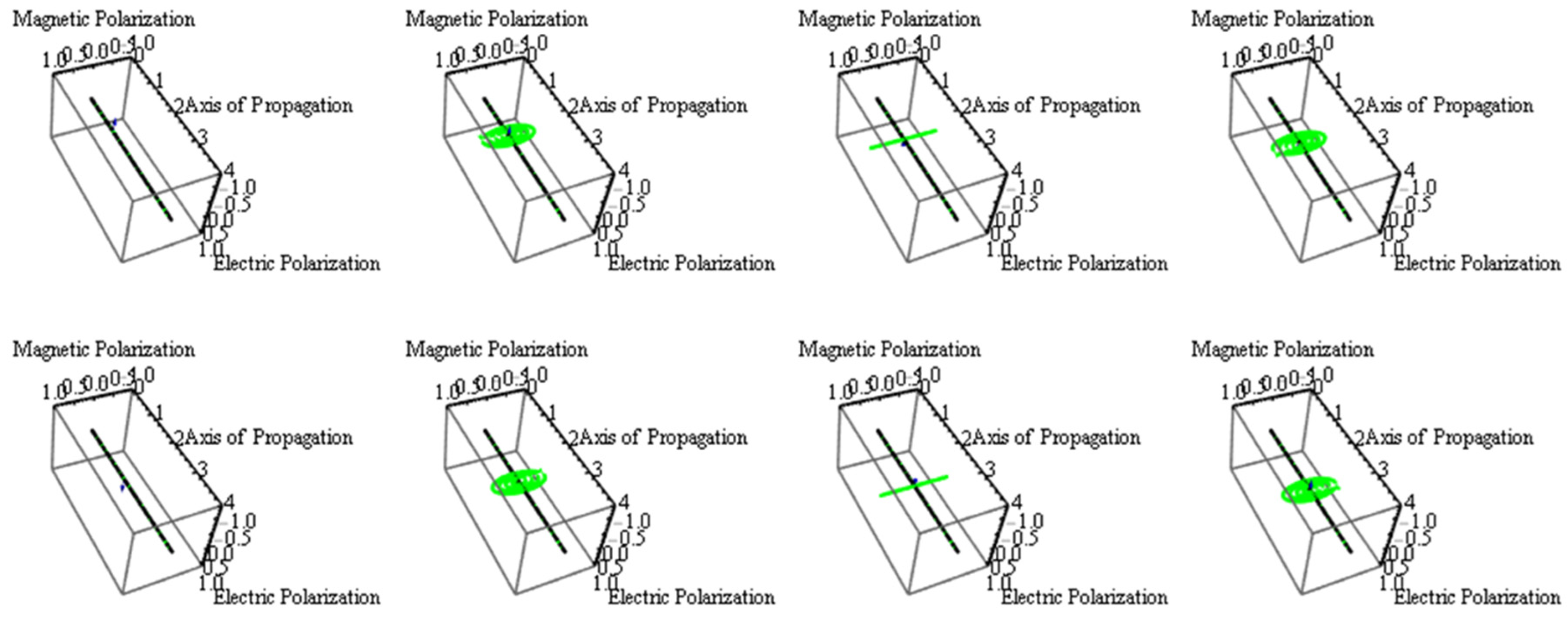
Figure 5.
Phasor diagram that represents the phase difference between the magnetic (green) and electric (blue) fields in electromagnetic waves propagating in free space. The images were captured every 1/8 of a wavelength from a .gif.
Figure 5.
Phasor diagram that represents the phase difference between the magnetic (green) and electric (blue) fields in electromagnetic waves propagating in free space. The images were captured every 1/8 of a wavelength from a .gif.
Disclaimer/Publisher’s Note: The statements, opinions and data contained in all publications are solely those of the individual author(s) and contributor(s) and not of MDPI and/or the editor(s). MDPI and/or the editor(s) disclaim responsibility for any injury to people or property resulting from any ideas, methods, instructions or products referred to in the content. |
© 2025 by the authors. Licensee MDPI, Basel, Switzerland. This article is an open access article distributed under the terms and conditions of the Creative Commons Attribution (CC BY) license (http://creativecommons.org/licenses/by/4.0/).
Copyright: This open access article is published under a Creative Commons CC BY 4.0 license, which permit the free download, distribution, and reuse, provided that the author and preprint are cited in any reuse.


