
Submitted:
11 August 2024
Posted:
13 August 2024
You are already at the latest version
Abstract
Maxwell's equations accurately describe the propagation of electromagnetic (EM) waves. However, the conventional formulation implies invariance to observers, posing challenges in explaining how the wave is perceived by different observers. For example, Doppler effect shows that observers perceive the same EM wave differently.By employing mathematical transformations, we derive a general form of Maxwell’s wave equations by incorporating a "time scaling" factor to account for observer perception. The original form is shown to be a special case when static. The Doppler effect and Sagnac effect are directly derived from Maxwell’s equations. All the results are consistent with established experiments.Our findings offer a fresh perspective, promising a deeper understanding and unification of EM phenomena. We extend Maxwell’s equations to describe not only the propagation of an EM wave, but also how it will be measured by different observers, say, antennas.
Keywords:
Maxwell equations
; Doppler effect
; Doppler radar
; Electromagnetic propagation
; Wave functions
; Sagnac effect
1. Introduction
Maxwell’s equations [1] provide a comprehensive description of EM wave propagation. What is missing from the picture is how an EM wave will
be perceived by different observers. Different observers will measure the same EM wave differently, for example, Doppler effect [2,3] shows that the same EM wave will be measured at different frequencies. While the frequency of the original EM wave doesn’t change after emission, the frequency “as measured” varies for different observers. Hence, Maxwell’s equations in current form only describe the EM wave “as propagated” but not “as measured”. This paper mathematically derives a general form of Maxwell’s equations which also describe the EM wave “as measured” by the observer.
The key to understand the difference between “as propagated” and “as measured” is the concept of “time scaling factor”, which explains the phenomenon: when an observer moving away from a clock, the clock appears ticking slower and when the velocity approaches , he will see the clock coming to a stall. If he compares the observed clock with his own clock, he will see a “time scaling factor”, which is due to the asymmetry between the light emission time at the light source and the observed time by the observer, and mathematically represented as . A formula for is mathematically derived in Asymmetry Theory [5]. The well-established principle of the constancy of the velocity of light [4] can be mathematically represented as . Based solely on this equation without any other assumption, a comprehensive set of results was derived through pure mathematics, named Asymmetry Theory [5,6,7].
The time in original Maxwell’s equations represents the clock for propagation. If we substitute it with the observer’s clock, i.e. , a generalized form of Maxwell’s equations for moving observer is mathematically derived in [5]. The transformed Maxwell’s equations are shown covariant for different observer reference frames in [5] and the original form of Maxwell’s equations is just a special case when .
In this paper, we further extend the case to also include the motion of the EM emitter. A general form of Maxwell’s equations is mathematically derived, and the original form is just a special case when the observer and emitter are static. Its solution demonstrated that the light velocity to observers is independent of the motion of the emitter, which demonstrates the principle of constancy of light velocity. The Doppler effect and Sagnac effect [10] are mathematically derived from the solution. A summary of the solutions of general equations in special cases is shown to be in harmony with all established experiments.
This paper is organized as follows:
Section II introduces the notations and background of the time-scaling factor.
Section III introduces how to mathematically transform the original Maxwell’s equations by substituting the time with .
Section IV presents the mathematical transformation of a general form of Maxwell’s equations for observers and the derivation of Doppler effect and Sagnac effect.
2. Notations and Background
2.1. Notations
Define as the emission time of a light; as the origin of the light when emitted at ; as the time an observer observed the light from ; as the position of at . Define as the velocity of the observer relative to at and as the velocity of the emitter relative at . Figure 1 also shows key angles for the velocity of light, .
2.2. Principle of Constancy of the Velocity of Light
Principle 1: In empty space, the light always propagates with a velocity . independent of the state of motion of the emitting body [4].
Principle 1 can be mathematically represented as:
This paper is solely based on the mathematical derivation from equation (1) without any other assumptions.
2.3. The Formula of
Perform an inner product of both sides of (3), we have:
Differentiate both sides as to and reorganize:
Let denote the unit vector in , we have:
Finally, the formula of time scaling factor [5] is:
When are constant and , (2) reduces to:
3. Maxwell Wave Equations for Observers
In this section, we introduce how to mathematically transform and solve the Maxwell wave equations for observers in [5].
3.1. Maxwell Wave Equations for Observers
Let’s consider a reference frame that the wave emitter is static to the wave origin, i.e. . The clock of the wave propagation, i.e. t, is in the same scale as the clock of the light emitter, i.e. . (4) can be written as:
By solving this equation (6), the wave propagation velocity is constant , consistent with Principle 1.
From the perspective of an observer, only the time it detects the light, i.e. , can be used to measure the wave propagation. Assume an observer with a velocity along the direction of the wave propagation. From equation (3), since , we have
Substitute with in (6), we have:
Similarly,
(8), (9) are the Maxwell wave equations as to an observer, which are mathematically equivalent to the original equations, simply in another form using for the observer’s perspective. They are shown covariant for different observer reference frames in [5]. When , they reduce to the original Maxwell’s equations.
3.2. Solution and Derivation of Classical Doppler Effect
The Doppler effect [2] is the change in frequency of the light to an observer who is moving relative to the light source, which is mathematically derived in [5] from solving Maxwell’s equations for observers (8), (9). The general solution to (8) is a linear superposition of waves of the form. Let
where is the frequency observed by the observer, is the wave vector and is the wavenumber. From (8), shall satisfy:
Hence, the wave propagation speed is:
The observed wave frequency is:
Since the emission wave frequency is , we have:
which is the same formula as the classical Doppler effect.
In summary, the formula of Doppler effect can be mathematically derived from the Maxwell wave equations for observers, which validates its physical correctness.
4. General Maxwell’s Equations for Observers
Now let’s consider the general case that both EM wave emitter and observer are moving. As Doppler effect shows the motion of the emitter also impacts how an observer measures the EM wave. This section will mathematically derive a general Maxwell’s equations for observers, which describe how the motions of emitter and observer impact the measurement of the EM wave.
4.1. General Maxwell’s Equations for Observers
First, let be the frame in which the EM wave emitter always stays in the center. Assuming are constant , we define:
and transfer to a new frame , in which the light origin is static. Hence, in this frame, the original Maxwell’s equations apply:
It follows:
We have:
Substitute with using ,we have:
(16) is the general form of Maxwell’s equations for observers. Similarly, we can get the same wave equation for the magnetic field .
4.2. Principle of Constancy of the Velocity of Light
Consider the simpler case where a polarized uniform plane wave propagates along the x direction, and (16) becomes:
The general solution to (16) is a linear superposition of waves. Let the solution be:
From (16), shall satisfy:
We have:
It is important to note that (17) shows the EM wave speed to any observer is independent of the motion of emitter , which clearly demonstrates the principle of constancy of the velocity of light [4].
Further note that in (17) is for one-way, which currently is considered un-measurable. The round way light speed can be calculated as:
Hence, the round-trip light speed always approximates if , which is consistent with experiments.
4.3. Derivation of Doppler Effect
From (17), we have the observed wave frequency as:
To get the emission wave frequency , we need to use the equation (15) with emission timing , which can be written as:
Solving (20) similarly, we have:
Hence,
Finally, combine (19) and (21) and we have:
So, we mathematically derived the same formula of traditional Doppler effect from the solution of the general form of Maxwell’s equations.
4.4. Reduced Forms and Solutions in Special Cases
The general Maxwell’s equations for observers (17) are mathematically transformed from the original equations. So, they are mathematically equivalent, and the general form reduces to the original form when ==0. Table 1 lists the reduced form and solution of Maxwell’s equations in some exemplary special cases.
In scenario 2, 0 =0, the solution shows that the EM wave speed is constant independent of the motion of the emitter, i.e. , which is consistent with the principle of constancy of the velocity of light.
In scenario 3, = 0, i.e. the emitter and observer are relatively static, the solution shows there is no Doppler effect, which is consistent with experiment.
Currently, many formulas are required to describe Doppler effect in different scenarios, for example, the scenario of moving emitter requires a different formula than the scenario of moving observer. But this general Maxwell’s equations provide a unified solution that is consistent with experiments in all scenarios.
4.5. Derivation of Sagnac Effect
The Sagnac effect [10] shows that two light beams, sent clockwise and counterclockwise around a closed path on a rotating disk, take different time intervals to travel the path, which contradicted the assumption that the light velocity is independent of the motion of the observer. Special Relativity attributed this contradiction to the rotating/accelerating frame [4,16]. Sagnac effect can be extended to a FOG [11] with
where is the detector speed, is the path length.
The phase variation of a light wave over the propagation path is given by:
where is the wave number. Use + and – distinguish the two light beams, we have the phase difference in the interferometer as:
From (19), it follows that:
Since this is the scenario3 in Table 1,
We have:
Since , hence
Since , finally we have:
which is the same formula of Sagnac effect as (23). So, we mathematically derived the same formula of Sagnac effect from the solution of Maxwell’s equations.
5. Conclusion
Maxwell’s equations in traditional form describe EM wave from the propagation perspective, where the time represents the propagation clock. Through mathematical transformation, a general form of Maxwell’s equations is derived to describe the EM wave from observer’s perspective by incorporating the time-scaling factor, i.e. using each observer’s own clock . The traditional form is just a special case when static. The solution of this general form of Maxwell’s equations is consistent with all established experiments. The formulas of classical and transverse Doppler effect and Sagnac effect can be directly derived from the solution, further confirming its physical validity. This result offers a comprehensive perspective of EM phenomena for both propagation and observers. One application is to predict the measurement of EM waves by a moving observer, say radar, and leverage it to improve design and performance.
References
- J. Maxwell, “A Dynamical Theory of the Electromagnetic Field,” Philos. Trans. R. Soc. Lond. 155, 459-512 (1865).
- C. Doppler, “Beiträge zur fixsternenkunde,” Prague: G. Haase Söhne, 69 (1846).
- Bélopolsky, “On an Apparatus for the Laboratory Demonstration of the Doppler-Fizeau Principle”, ApJ. 13, 15 (1901).
- Einstein, “On the Electrodynamics of Moving Bodies”, Annalen der Physik, 17, 891-921 (1905).
- Q. Chen, “Asymmetry Theory mathematically derived from the principle of constant light speed”. [CrossRef]
- Q. Chen, “Design of Experiments for Light Speed Invariance to Moving Observers”. [CrossRef]
- Q. Chen, “A mathematically-derived unified formula for Time-Varying Doppler effect, Cosmological red-shift and Cherenkov radiation”, Optica Open, doi.org/10.1364/ opticaopen.25612566.v1 (2024).
- D.C. Champeney et al., “Absence of Doppler shift for gamma ray source and detector on same circular orbit.,” Proc. Phys. Soc. 77, 350 (1961). [CrossRef]
- H. W. Thim, “Absence of the relativistic transverse Doppler shift at microwave frequencies,” IEEE Trans. Instr. Measur. 52, 1660-1664 (2003).
- G. Sagnac, “L’ether lumineux demontre par l’effet du vent relatif d’ether dans un interferometre en rotation uniforme,” C. R. Acad. Sci. Paris 157, 708 (1913).
- R. Wang et al., “Modified Sagnac Experiment for Measuring Travel-Time Difference between Counter-Propagating Light Beams in a Uniformly Moving Fiber,” Physics Letters A. 312 (1–2): 7–10 (2006). [CrossRef]
- S.J. Barnett, “On Electromagnetic Induction and Relative Motion,” Phys. Rev. 35, 323 (1912). [CrossRef]
- K. Brecher, “Is the Speed of Light Independent of the Velocity of the Source?” Phys. Rev. Lett., 39, 1051 (1977). [CrossRef]
- T. Alvaeger et al., “Test of the second postulate of special relativity in the GeV region,” Phys. Lett. 12, 260 (1964). [CrossRef]
- G. C. Babcock et al., “Determination of the Constancy of the Speed of Light,” J. O. S. A. 54, 147 (1964).
- P. Langevin, “Sur la théorie de la relativité et l'expérience de M. Sagnac,” Comptes Rendus. 173: 831–834 (1921).
Figure 1.
Notations for light velocity [5].
Figure 1.
Notations for light velocity [5].
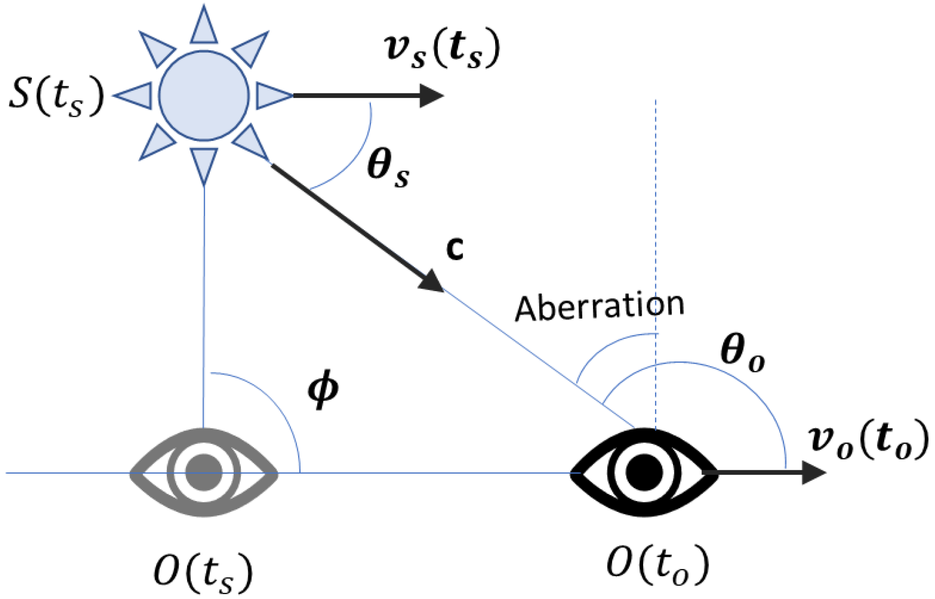

Table 1.
Reduced forms of general Maxwell’s equations in special cases and corresponding solutions.
| Scenarios | Maxwell Equations for observer | ||
| General equation for the motion of observer and source | |||
| ==0Original Maxwell’s equation | 1 | ||
| 20 =0Principle of constant light speed | |||
| 3.= 0Observer static to source | 1 | ||
| 4=0 0Source fixed to origin |
a Gaussian units are the same as cg emu for magnetostatics; Mx = maxwell, G = gauss, Oe = oersted; Wb = weber, V = volt, s = second, T = tesla, m = meter, A = ampere, J = joule, kg = kilogram, H = henry.
Disclaimer/Publisher’s Note: The statements, opinions and data contained in all publications are solely those of the individual author(s) and contributor(s) and not of MDPI and/or the editor(s). MDPI and/or the editor(s) disclaim responsibility for any injury to people or property resulting from any ideas, methods, instructions or products referred to in the content. |
© 2024 by the authors. Licensee MDPI, Basel, Switzerland. This article is an open access article distributed under the terms and conditions of the Creative Commons Attribution (CC BY) license (http://creativecommons.org/licenses/by/4.0/).
Copyright: This open access article is published under a Creative Commons CC BY 4.0 license, which permit the free download, distribution, and reuse, provided that the author and preprint are cited in any reuse.


