Maxwell and Artificial Intelligence: Preliminary QED Models of AI (LLM) Dynamics

1. Maxwell Vector Potential

1.1. Consider a Verbal Task A for LLM

Assume A has a family of n features. Note that the task A may involve more than n features, and together these residues features are treated as gauge freedom later. In LLM, the transformer generates a weight for each of n features, and embeds A as vectors. This step is called embedding. Solving a task may involve many rounds of embeddings, each updates the vector space to certain extensions.

Definition 1. As an LLM procedure, the transformer embeds a verbal task to a vector space, denoted by $A_{\mu }$. Call $A_{\mu }$ the Maxwell vector potential; it is also called the Maxwell field. In other words, a verbal task brings in the external potential. $A_{\mu }$ can be characterized by exterior form as 1-form, which stands for $f\left(x\right)dx$.

In LLM, gradience descent is a major technique for deep learning. The gradience, $F_{\mu \upsilon }$, can be characterized as 2-form in terms of the exterior form. The relation between $A_{\mu }$ and $F_{\mu \upsilon }$ is as below.

Definition 2. The gradience of $A_{\mu }$, denoted by $F_{\mu \upsilon }$. We have,

$$F_{\mu \upsilon }={\partial }_{\mu }{A}_{\nu }-{\partial }_{\nu }{A}_{\mu }$$

In gauge field theory, $F_{\mu \upsilon }$ stands for the gauge field strength; it is a density function.

There are three paths to build QED models for LLM. [1] The first path is by interactions of a charge field with Maxwell field. The second path is by the interactions of a spinor field (Direc field) with Maxwell field. The third path is by the interactions of Klein-Gordon field with Maxwell field. In this theoretical note, we only consider the first two paths, i.e., we follow the first path and the second path to build QED models for LLM framework.

1.2. From the Angle to the Dynamic Phase

In LLM, the inner product is introduced in the vector space. Thus, from one vector can produce another vector and the superposition of two vectors. Between any two vectors, there is an angle which is currently called the distance. This is exactly the illusion effected H. Wyle that delated him from establishing gauge field theoretic dynamics. To correct it, we have,

Definition 3. The angle between two potential vectors is defined as the dynamic phase. Thus, from one potential state $\psi$ to another potential state ${\psi }^{\prime }$can be represented as

$$\psi \to {\psi }^{\prime }=e^{i\theta }\psi$$

where $\theta$ stands for dynamic phase. This is the key move from LLM to AI dynamics. This is called the gauge transformation of the first kind at the global level. This gauge transformation also requires keeping the transformation conformal at the local level, where $\theta$is no longer an any given constant but a function $\theta$(x). The gauge transformation at the local level is called the gauge transformation of the second kind. The gauge principle says that if the gauge transformation of the first kind does not hold, then the gauge transformation of the second kind can not be hold. In order to achieve the local gauge symmetry, it needs to introduce new notions, namely, covariate derivative and gauge field. We will develop this point latter.

2. Charge Field Interacts with Maxwell Potential

Dynamic analysis is the sourced analysis, and this source is called the charge. We have

Postulate 1. The LLM tasks carry the task charge, denoted as E. A task can be characterized by a family of features. By Anne Treisman [2], the integration of these features demands attention. Call this integration the charge potential and denote it as $\varphi$.

To solve a task demands some intentions and solving a task demands a number of intelligence factors, such as reasoning, learning, understanding, integrating, etc. We have

Postulate 2. Let $A_i$ are intelligence factors. The integration of $\left(A_i\right)$ is defined as the intelligence potential, denoted by $\overrightarrow{A})$.

Definition 3. The notion of AI vector potential is defined as a unit with two components,

$$A_{AI}=\left[\varphi ,-\overrightarrow{A}\right]$$

This idea can be seen as a Platonic version of Maxwell vector potential; it is a field. In quantum field theory, the charge is characterized as a field. Here it is called the task-charge field. denoted as TCF. The TCF interacts with $A_{AI}$ yields a dynamic model, logically skin to that an electric field interacts with the Maxwell potential field yields quantum electrodynamics (QED).

3. Spinor Field Interacts with Maxwell Potential

3.1. Wyle Spinor

We make a clear distinction of the human intelligence ($\mathsf{\alpha })$and the machine intelligence ($\mathsf{\beta })$. Further, we make a mathematical trivialization treatment such that $\mathsf{\alpha }$ and $\mathsf{\beta }$ are orthogonal:

$${\delta }_{\alpha \beta }=\left\{\begin{array}{c}1, \alpha =\beta \\ 0, \alpha \ne \beta \end{array}\right.$$

Now we define $\mathsf{\alpha }$ as the intelligence demand ($D_{\mathsf{\alpha }})$ and $\beta$ as the intelligence supply $\left(S_{\beta }\right)$. For an any given task $\mathsf{\phi }$, we have

Definition 5. $e^{-}=\left[ D_{\mathsf{\alpha }} , {\mathsf{\phi }}^{-}\right]$, and $e^{+}=\left[ S_{\beta } , {\mathsf{\phi }}^{+}\right]$.

The above definitions can be characterized as a Wyle spinor below,

$$\psi =\left(\begin{array}{c}{\psi }_1\left(=e^{-}\right)\\ {\psi }_2\left(=e^{+}\right)\end{array}\right)$$

3.2. Dirac Spinor

In the neural network for deep learning, the hidden layers indicate that both human intelligence and machine intelligence hesitate. This kind of intellectual hesitation reflects a certain kind of rationality. Such a hesitation is characterized as spin, which has two eigenstates, spin up ($\uparrow )$or else spin down ($\downarrow$); thus, in a sense, both $e^{-} \mathrm{and} e^{+}$ spin ½. This can be seen at the activating stage in the architecture of neural network, which returns only 0 or 1. We need hidden layers to calibrate and update neural weights (probabilities), during which the intelligent processes experience all possible superpositions of the two eigenstates. Taking spins into account, the Wyle spinor is developed into Dirac spinor, represented as below，

$$\psi =\left(\begin{array}{c}\begin{array}{c}{\psi }_{1 }\left(=e^{-}\uparrow \right)\\ {\psi }_2 \left(=e^{-}\downarrow \right)\end{array}\\ \begin{array}{c}{\psi }_3 \left(=e^{+}\uparrow \right)\\ {\psi }_{4 }\left(=e^{+}\downarrow \right)\end{array}\end{array}\right)$$

3.3. Photon Field

In quantum field theory, the Maxwell field is the photon field, which is denoted by $\mathsf{\lambda }$. In market dynamics [3], the phone field is used to model the price field. Here, in LLM, the photon field is used to mode the cost function of neural network. In quantum field theory, all particles are described as a field, and a field is characterized as an operator. In addition, all the particles have its life span, they are created and annihilated. We need to introduce the creation operators here, the creation operator (${\widehat{a}}^{†}$) and the annihilation operator ($\widehat{a})$. They are adjoint operators. A simple interaction is that a pair of $e^{-}$ and $e^{+}$are created and they fly in inverse directions to each other. Then, both are annihilated by creating a photon field $\mathsf{\lambda }$. This process can be pictured by Feynman diagram shown in Figures 1,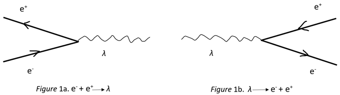

One may start from here to develop a detailed model of LLM skin to spinor electrodynamics.

4. Wavefunction and Measurement Problem

The major processes in LLM learning/training are not directly observable; thus, it should be characterized as the U-procedure (Unitary procedure) of a wavefunction [4]. Hence, the probability used in LLMs should be Born probability. Note that at the activating stage of the neural network, the feature weights are converted to 0 or 1; this is actually a Yes/No measurement [5], which is called the R-procedure (reduction procedure). This reflects the measurement problem in quantum physics. Yang [6] proposed a unified account of the U-Procedure and the R-Procedure as an alternative solution of the measurement problem.

References

- Wang, Z. Elementary Quantum Field Theory; Peking University Press (China), 2008. [Google Scholar]
- Treisman, A. A Feature-Integration Theory of Attention. Cognitive Psychology 1980, 12, 97–136. [Google Scholar] [CrossRef] [PubMed]
- Yang, Y. Principles of Market Dynamics: Economic Dynamics and Standard Model (II). Science, Economics, and Society 2022, 40, No. 5 (China). [Google Scholar]
- Penrose, R. The Road to Reality: A Complete Guide to the Laws of the Universe; Random House, Inc.: New York, 2005. [Google Scholar]
- von Neumann, J. Mathematical Foundations of Quantum Mechanics; Princeton University Press: Princeton, New Jersey, 1955. [Google Scholar]
- Yang, Y. The revised Schrödinger equation as a solution of measurement paradox: A unified model of the U-procedure and the R-procedure. 2024. [Google Scholar] [CrossRef]
Disclaimer/Publisher’s Note: The statements, opinions and data contained in all publications are solely those of the individual author(s) and contributor(s) and not of MDPI and/or the editor(s). MDPI and/or the editor(s) disclaim responsibility for any injury to people or property resulting from any ideas, methods, instructions or products referred to in the content. |
© 2025 by the authors. Licensee MDPI, Basel, Switzerland. This article is an open access article distributed under the terms and conditions of the Creative Commons Attribution (CC BY) license (http://creativecommons.org/licenses/by/4.0/).
Copyright: This open access article is published under a Creative Commons CC BY 4.0 license, which permit the free download, distribution, and reuse, provided that the author and preprint are cited in any reuse.