Submitted:
25 April 2025
Posted:
30 April 2025
You are already at the latest version
Abstract
This paper introduces a novel control technique for embedded systems based on error-dependent sampling, referred to as Error-Dependent Sampling Control (EDSC). Unlike traditional control methods, which rely on fixed sampling intervals, EDSC dynamically adjusts the sampling rate based on the magnitude of the error signal. By incrementing or decrementing the control signal by a fixed step size of 1 when an error is present, and maintaining the output when the error is zero, this approach minimizes computational complexity. The sampling frequency increases as the error grows, resulting in faster response times during larger errors and fewer updates during smaller errors, thus optimizing system performance and reducing energy consumption. The proposed method utilizes timer interrupts, making it well-suited for embedded systems with limited processing power. The advantages of EDSC are highlighted through its efficiency in both energy consumption and computational load, particularly for low-power microcontrollers. This technique is compared with traditional control methods such as PID and other variable sampling approaches, demonstrating its potential for real-time applications in embedded control systems.
Keywords:
adaptive control
; variable-rate sampling
; proportional control
; DC motor control
; embedded systems
1. Introduction
Control systems are central to a wide range of applications, from industrial automation to embedded systems. Traditional control techniques, such as Proportional-Integral-Derivative (PID) controllers, have long been the standard in many systems, offering a reliable and straightforward method for maintaining desired system behavior. However, as systems become more complex and embedded in resource-constrained environments, the need for more efficient control methods becomes increasingly important. In particular, the computational and energy demands of traditional fixed-sampling control methods may pose challenges for microcontrollers with limited processing power.
In response to these limitations, various approaches have been proposed to optimize control performance by adjusting the sampling frequency based on system requirements. Methods like Event-Triggered Control (ETC) [1,2], Self-Tuning Sampling [3,4], and Pulse Frequency Modulation (PFM) [5,6] offer dynamic sampling strategies that improve efficiency by sampling more frequently when the system is experiencing significant changes or errors and less frequently when the system is stable. These methods aim to strike a balance between system performance and resource consumption, but they often introduce complexities in computation, particularly in real-time embedded systems [7,8].
This paper introduces a novel control technique, EDSC, which dynamically adjusts the sampling frequency based solely on the magnitude of the error. The core idea of EDSC is simple: when an error is present, the controller increments or decrements the control signal by a fixed step size of 1 and when the error is zero, the output remains unchanged. The control signal update rate (or simply the sampling rate) is adjusted such that larger errors result in more frequent updates, while smaller errors lead to less frequent updates. This dynamic behavior enables the controller to respond quickly to significant changes in the system, while conserving resources when the system is stable.
The proposed EDSC method is implemented using timer interrupts, making it particularly well-suited for embedded systems with small-core microcontrollers that are limited in processing power. By eliminating the need for complex integration or differentiation calculations, EDSC provides a computationally efficient alternative to traditional control methods. Additionally, the dynamic sampling behavior ensures that system resources are used more effectively, particularly in real-time applications with stringent energy and processing constraints.
In the following sections, a comprehensive analysis of EDSC is provided, comparing it to existing control strategies and highlighting its applications in embedded systems. The advantages and challenges associated with implementing this approach in real-world scenarios are further examined.
The paper is structured as follows: Section II presents a literature review and the mathematical modeling of well-established control techniques that incorporate variable sampling, along with an introduction to the EDSC. Section III formally defines the mathematical modeling of the proposed EDSC technique. Section IV details the implementation methodology of EDSC on microcontrollers, addressing practical considerations. Section V refines the system’s transfer function, providing deeper insights into its behavior. Section VI presents MATLAB-based simulations and a Lyapunov stability analysis to assess system performance. Section VII demonstrates a microcontroller-based implementation of EDSC, including firmware design and experimental validation. Finally, Section VIII concludes the paper with a summary of findings and potential directions for future research.
2. Literature Review and Modeling of Variable Sampling Techniques
2.1. Most Common Variable Sampling Techniques
In control systems, specifically in discrete systems like digital PID controllers, a fixed sampling period is typically used for the computation of error and tuning of constant parameters [1,9]. This consistent sampling allows for predictable integration and differentiation over time. However, there are advanced techniques that use variable sampling instead of a fixed period to optimize system performance [2,7].
Here are some of the techniques that use variable sampling:
-
*Sampling Trigger: Sampling occurs when a certain error threshold is exceeded or a specific event is detected.*Advantages: This reduces unnecessary computation, saving energy and bandwidth. It only samples when needed, optimizing the control process.*Disadvantages: It may introduce unpredictability in system response due to the irregularity of sampling.*Applications: Networked control systems, IoT, and systems with limited communication bandwidth.
-
*Sampling Trigger: The sampling period adapts to the system’s dynamics or state. It changes based on error magnitude, system speed, or performance requirements.*Advantages: More efficient computation as the sampling rate increases when there are large changes in system dynamics.*Disadvantages: Requires real-time analysis of the system’s state, which can be computationally expensive.*Applications: Automotive systems, adaptive controllers, and energy-efficient systems.
-
*Sampling Trigger: The next sampling instant is predicted based on a model of the system, compensating for time delays.*Advantages: This approach can improve stability and control performance in systems with inherent delays.*Disadvantages: Requires an accurate model of the system, which may not always be available or reliable.*Applications: High-speed control systems, nonlinear systems, or systems with communication delays.
-
*Sampling Trigger: The sampling rate varies depending on the system state, such as velocity, acceleration, or other dynamic variables.*Advantages: Adjusting sampling based on system state allows for better responsiveness and performance, particularly in fast-changing systems.*Disadvantages: Requires real-time state estimation and may not be suitable for all systems.*Applications: Robotics, motion control, and aerospace systems.
-
*Sampling Trigger: Sampling is based on a mathematical model that predicts when the next sampling is required, optimizing for performance or energy usage.*Advantages: This approach minimizes unnecessary updates and is energy-efficient.*Disadvantages: It is more complex to implement, requiring an accurate model and real-time computations.*Applications: Embedded systems, low-power control applications, and systems with limited resources.
-
Bang-Bang Control (On-Off Control) [1]*Sampling Trigger: The control action switches fully ON or OFF based on a predefined error threshold.*Advantages: Simple and cost-effective with fast response, especially for systems where precise control is not necessary.*Disadvantages: Can cause oscillations or instability because of the lack of smooth control; not suitable for systems that require fine control.*Applications: Thermostats, motor drives, basic automation systems.
-
*Sampling Trigger: The sampling rate adapts based on the magnitude of the error, adjusting the pulse frequency to maintain control.*Advantages: Energy-efficient, as it dynamically adjusts the control signals according to the system’s needs.*Disadvantages: Less precise than Pulse Width Modulation (PWM), which can lead to less accurate control; requires careful tuning and design.*Applications: Power electronics, switching regulators, and embedded control applications.

Table 1.
Comparison of Variable Sampling Techniques and Related Control Methods.
| Technique | Sampling Trigger | Advantages | Disadvantages | Common Applications |
|---|---|---|---|---|
| Event-Triggered Control (ETC) | Sampling occurs when an error threshold is exceeded | Reduces unnecessary computations, saves bandwidth | May introduce unpredictable delays | Networked control systems, IoT, industrial automation |
| Self-Tuning Sampling (Adaptive Sampling) | Sampling time adapts based on system dynamics | Efficient computation, better transient response | Requires real-time analysis of system state | Automotive control, energy-efficient systems |
| Time-Delay Control (TDC) | Predictive model determines next sampling instance | Compensates for delays, improves stability | Requires an accurate model of the plant | High-speed or nonlinear control systems |
| State-Dependent Sampling | Sampling varies with system state (e.g., velocity, acceleration) | Adjusts to dynamic changes, improves performance | Requires real-time state estimation | Robotics, motion control, aerospace |
| Model-Based Variable Sampling | Uses a mathematical model to optimize sampling | Energy-efficient, minimizes unnecessary updates | Complex implementation, requires a reliable model | Embedded systems, low-power control applications |
| Bang-Bang Control (On-Off) | Control action switches fully ON or OFF based on threshold | Simple, cost-effective, fast response in some systems | Can cause oscillations, not precise | Thermostats, motor drives, basic automation |
| Pulse Frequency Modulation (PFM) | Pulse frequency adapts based on error magnitude | Energy-efficient, dynamic response adapts to needs | Less precise than PWM, requires careful design | Power electronics, switching regulators, embedded control |
2.2. Most Common Control Methods Modeling
2.2.1. Proportional-Integral-Derivative (PID) Control
PID control remains the most widely used control algorithm in industrial applications due to its simplicity and effectiveness [14]. The control law combines three distinct actions:
where is the tracking error, is the proportional gain, the integral gain, and the derivative gain. The proportional term responds to present error, the integral term eliminates steady-state error through historical error accumulation, and the derivative term anticipates future trends [9]. In frequency domain, the PID transfer function is:
2.2.2. Bang-Bang Control
Also known as on-off control, bang-bang control represents the simplest nonlinear control strategy, characterized by:
where is a hysteresis band that prevents chattering. This discontinuous control law drives the system to its target by applying maximum effort in alternating directions [16]. While simple to implement, it causes persistent oscillations (limit cycles) around the setpoint:
where depends on system dynamics and delay [17]. Applications include thermostats, spacecraft attitude control [18], and systems with actuator saturation. Modified versions incorporate dead zones or adaptive thresholds to improve steady-state performance [19].
2.2.3. Pulse Frequency Modulated (PFM) Control
PFM is a nonlinear control strategy that modulates the switching frequency of actuator pulses based on system error, offering inherent efficiency advantages in power-constrained systems [10]. Unlike fixed-frequency PWM, PFM regulates energy delivery through variable timing between constant-width pulses:
where is the base frequency, K the modulation gain, and the sampled error. The binary control action follows:
with fixed pulse width . This produces a duty cycle , where , enabling proportional behavior through frequency-domain averaging [11]. PFM’s efficiency stems from reduced switching losses at light loads (), making it ideal for battery-powered systems [12]. However, variable-frequency operation introduces harmonic complexity requiring careful electromagnetic compatibility (EMC) design [13]. Recent implementations combine PFM with hysteretic current control for improved transient response:
where defines the high-error regime [6].
2.3. Contribution: Proposed EDSC Method
The EDSC method introduces a unique approach to discrete control systems by dynamically adjusting the control signal update rate (i.e. sampling frequency) based on the magnitude of the error, while keeping the control step size fixed at 1. The sampling period , is function of error, :
Unlike traditional control systems such as PID, where the sampling period is constant and the controller updates its output at regular intervals, the EDSC method varies the sampling rate according to the error magnitude (see Figure 1). This means that when the error is large, the system updates the control signal more frequently. Thus, the updated control signal, , is function of its previous value and the sign of the error:
This dynamic adaptation enables faster corrections in case of large errors while conserving computational resources when the error is small, leading to improved efficiency and responsiveness.
A key advantage of this method is its ability to operate with timer interrupts, which is particularly beneficial for embedded systems using small core microcontrollers. In these systems, computational power is often limited, and complex operations such as integration or differentiation are impractical due to the constraints of the microcontroller’s Arithmetic Logic Unit. EDSC eliminates the need for such computations by leveraging timer-based interrupts to control the sampling rate, simplifying the control process. This means that instead of performing complex mathematical calculations, the controller simply relies on timers to adjust the frequency of control updates based on the error magnitude. When the error is small, the method reduces the frequency of updates, preventing unnecessary computations and conserving power, which is especially important in battery-operated or energy-efficient systems. On the other hand, when large errors occur, the system increases the update frequency, enabling rapid corrections without the need for complex algorithms or additional hardware.
3. Mathematical Modeling of EDSC
In the context of EDSC, the control signal is represented by a PWM signal that is adjusted according to the error signal. PWM is widely used in embedded control systems to regulate power delivered to devices by varying the duty cycle of a rectangular wave signal.
For this system, the PWM signal is directly linked to the error , and the controller modifies the duty cycle based on the error value. The controller adjusts the PWM signal in such a way that the changes with a fixed step size of 1, depending on the sign of the error.
Let denote the Duty Cycle of the PWM signal at time step k. The PWM signal is modulated as follows:
where, is the maximum value of the control signal, which defines the upper limit of the duty cycle.
is adjusted by incrementing or decrementing the control signal based on the error signal. If the error is positive, the is incremented, and the duty cycle increases. Conversely, if the error is negative, is decremented, and the duty cycle decreases. When the error is zero, the duty cycle remains constant, and the control signal does not change. The duty cycle adjusts as:
Thus, while the frequency of the PWM signal remains constant, the variation of the duty cycle is dependent on the error, providing a dynamic control mechanism. This dynamic control adjusts the power delivered to the system faster when the error is large and less frequently when the error is small.
The EDSC technique adjusts the sampling period dynamically based on the magnitude of the error. The key equations governing the system are:
The control signal is updated with a fixed step size of 1:
where:
The sampling period is inversely proportional to the magnitude of the error:
where:
- is the maximum sampling period,
- C is a tunable constant that controls the rate of adaptation.
The next sampling instant is determined as:
4. Embedded System Implementation of EDSC
Timer is the major component used to calculate the EDSC control signal. Usually, even small core microcontrollers have timer interrupt events. The timer is incremented through a prescaler and generates interrupt on overflow. The incrementing speed of timers depends on the oscillating frequency of the chip.
The PIC16F886 microcontroller is used to implement EDSC using Timer0 interrupts. Assuming the PIC is running at an oscillating frequency (MHz) and the instruction time is (). Timer0 register is set based on the error magnitude.
4.1. Timer0-Based Sampling Period
Using Timer0 of the PIC16f886, the timer overflows after based on the following equation:
Since Timer0 is an 8-bit timer, . Assuming also that the PIC is running at 4Mhz, i.e. .
The equation becomes
where TMR0 is calculated as:
acts as a scaling factor, or proportional gain, that determines how the sampling period adapts to the error magnitude. It plays a similar role to the proportional gain, in a PID controller but affects the sampling rate instead of the control signal directly.
Substituting into Equation (1), becomes:
For a prescaler of 256, this simplifies to:
where 65536 represents the maximum sampling period .
It can be concluded from the above equation that affects the sampling time as:
- Increasing :→ Faster response, as larger errors lead to smaller (higher sampling frequency). However, too high may cause instability due to excessive sampling.
- Decreasing :→ Slower response, as the system updates less frequently even for large errors, leading to sluggish control.
On the other hand, the sampling frequency, can be represented as:
As shown in Figure 2, for , the sampling frequency is 15 Hz. This indicates that in the absence of error, the timer generates approximately 15 interrupts/overflows (i.e., 15 checks per cycle). However, when the error increases (e.g., ), the timer generates 17 overflows, corresponding to 17 increments of the duty cycle. This results in a faster response of the output.
The control signal is applied through PWM, where the is updated as:
The PWM frequency remains constant, but the duty cycle is updated dynamically at every sampling interval . The PWM duty cycle register, CCPRxL, is adjusted in steps:
It is also important to mention the effect of on the sampling frequency, . For example, for the same error of 30, the sampling frequency changes from 17 Hz (for ) to 23 Hz (for ).
As a summary of the implementation steps: The mathematical equations listed above are implemented in the microcontroller through the following steps:
- Setup the timer prescaler (256 as per Equation (2)).
- Measure error,
- Reload Timer0 as
- Adjust PWM duty cycle
- Wait for Timer0 interrupt and repeat step 2
This ensures that:
- The sampling time decreases as the error increases
- The PWM duty cycle changes in discrete steps based on the sign of the error
- The plant response adapts dynamically, improving efficiency
5. Refined Transfer Function Approximation of EDSC with DC motor
Approximating the transfer function of the EDSC system is challenging due to its nonlinear and time-varying nature. Since the sampling time depends on the error , the system is approximated using a continuous-time equivalent model.
5.1. Motor Dynamics and Control Law
The DC motor follows the standard first-order dynamics:
where:
- J is the moment of inertia (kg·m2),
- B is the viscous friction coefficient (N·m·s),
- K is the motor gain constant (rad/V·s),
- is the angular velocity (rad/s),
- u is the control signal (PWM or voltage applied to the motor).
Taking the Laplace transform:
The control law in discrete time is:
Unlike conventional discrete controllers that use a fixed sampling period, this system dynamically adjusts the sampling period based on the error magnitude:
To approximate the system as a sampled-data system with a fixed sampling rate, a nominal error is assumed:
Applying zero-order hold (ZOH) discretization, the discrete-time transfer function is approximated as:
which shows that the system behaves like a gain-scheduled discrete system, where varies with .
5.2. Continuous-Time Approximation with Delay
For small perturbations around , the sampling time variation can be approximated as:
This introduces a time-varying delay in the system response. The motor dynamics in the presence of delay can be approximated as:
Approximating using a first-order Taylor expansion:
Substituting this into the motor equation:
Taking the Laplace transform:
Solving for , the system can be approximated as a first-order system with a varying delay:
The delay term represents the nonlinear, error-dependent delay.
This refined model provides a mathematical foundation for understanding the impact of variable sampling on system behavior and can guide further tuning and stability analysis. The system’s stability can be analyzed using Lyapunov-Krasovskii methods for delay systems.
6. EDSC Matlab Simulation and Lyapunov Stability Analysis
6.1. Matlab Simulation Setup and Results
The adaptive control system was simulated in MATLAB to analyze its performance under two error sensitivity gains: and . The simulation results are presented in Figure 4 and Figure 5. The system comprised a DC motor with parameters:
- Moment of inertia: kg·m2,
- Viscous friction: N·m·s,
- Motor constant: rad/V/s.
The motor was tasked with tracking a reference velocity rad/s. The EDSC adjusted the control signal u in discrete steps () with saturation limits: and .
- Case 1 (): The system achieved a 95% settling time of s with an average sampling interval of s. However, steady-state oscillations persisted, with rad/s, due to discrete control adjustments.
- Case 2 (): The average sampling interval reduced to s, improving the transient response with a reduced settling time of s. However, the steady-state error remained unchanged ( rad/s), indicating that primarily affects transient behavior.
These results highlight a key design trade-off: increasing enhances transient performance but at the cost of increased interrupt events, whereas lower values conserve resources at the expense of marginally slower convergence.
6.2. Lyapunov Stability Analysis of the EDSC System
To analyze the stability of the EDSC system, Lyapunov’s Stability Theorem is used. A discrete-time system, , is stable if there exists a Lyapunov function such that:
1. for all and (Positive definite).
2. (Non-increasing function, ensuring energy dissipation).
3. If , the system is asymptotically stable (error converges to zero).
A suitable Lyapunov candidate function for this system is:
which is positive definite and represents the "energy" of the error.
evolves over time as:
From the control law equation presented in Equation (5), since the error updates based on the motor dynamics, it can be approximated as:
Substituting into of Equation (6) and expanding the expression:
The difference of Equation (7) is thus:
For stability, it is required to have , which simplifies to:
which ensures , meaning the system is globally asymptotically stable as long as:
- If is too large, the system updates too aggressively, leading to potential oscillations.
- If is too large, the system updates too slowly, making convergence slow.
- By ensuring , the system remains stable, and the error will eventually reach zero.
Based on the numerical values discussed previously, the maximum Ts is , means that the stability is satisfied as long as is lower than 2/0.065536 = 30.517. Thus, the stability condition ensures that the error-dependent sampling remains effective without causing instability.
7. EDSC Implementation Design and Experimental Results
7.1. Implementation Setup
The EDSC is implemented on the PIC16F886, an 8-bit microcontroller from Microchip. The main task is to control the speed of a DC motor (with unknown parameters) in conjunction with a Hall sensor. The system utilizes three timers and one external interrupt to achieve the computations defined in Equation (2) and Equation (4).
- External interrupt handler is responsible for counting the pulses generated by the motor shaft’s Hall sensor.
- Timer1 interrupt handler is responsible for measuring a one-second interval, during which the accumulated Hall sensor pulses are utilized to compute the real-time motor shaft speed. Consequently, the actual speed is updated at a fixed interval of one second. In the implemented prototype, the Hall sensor generates 8 pulses per revolution, thus, Timer1 is configured to trigger an interrupt every seconds (i.e., 125 ms), enabling a more frequent update of the actual speed.
-
Timer2, in conjunction with the Capture/Compare/PWM module, is used to generate the PWM control signal.
Additionally, the main code manages UART data transmission, sending real-time values for the desired speed, actual speed, interrupt frequency, and PWM duty cycle. These parameters are graphically visualized through a C#-based application specifically developed for this purpose.
7.2. Experimental Results
The EDSC controller is used to drive a DC motor at various speeds (specified in the code). The desired speeds are provided as step and ramp inputs. The results are presented in Figure 10, Figure 11, and Figure 12 for , 5, and 10, respectively.
The experimental result curves illustrate the motor speed response in relation to the desired speed (displayed in the upper window), the sampling frequency as defined in Equation (3) (shown in the lower left-hand side window), and the PWM duty cycle as described in Equation (4) (shown in the lower right-hand side window). The collected 600 points corresponds to 35 seconds, i.e., time between sample is around 58 ms (PIC sends a set of data every 58 ms).
Figure 10 shows the response for . The motor response is slower, but it successfully follows the desired speed with zero error.
In Figure 11, the motor responds more quickly for . It is evident that the sampling frequency exhibits spikes due to the error being multiplied by 5.
Figure 12 illustrates the motor’s aggressive response for . In all cases, the response demonstrates good tracking of both the step and ramp inputs with zero error.
Hardware Limitations: From Eq. (2), it is evident that the sampling period must always remain positive. This condition implies that the term must be strictly less than 65536; otherwise, becomes negative, leading to instability in the timer operation.
To ensure that remains positive, the constraint must be satisfied. Consequently, the curves showing the sampling frequency are limited to a maximum value of 255.
For example, for , as illustrated in Figure 10, the maximum allowable error is . Any value above 63 must be rectified to 63. This corresponds to a sampling period of and a maximum sampling frequency of , which results in 976 increments of the PWM duty cycle. However, since the PWM register is limited to a maximum value of 255, constraints are imposed on the control algorithm. As a result, in the firmware implementation, the slope value is capped at 250, and the CCPRxL register is also limited to 250, as shown in the snippet code of Figure 7. It is important to highlight that the actual speed is updated every 125 ms, as determined by the Timer1 interrupt previously discussed. This periodic update allows for a direct observation of error reduction, resulting in a rapid adjustment of the sampling frequency, which is one of the major advantage of the proposed controller.
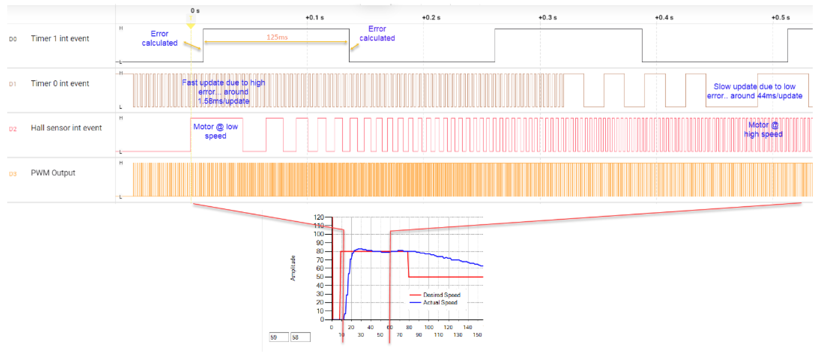
To facilitate real-time monitoring of the microcontroller’s behavior, additional debugging mechanisms were integrated into the firmware. Specifically, each interrupt event is mirrored by a state transition on dedicated digital output pins, enabling precise tracking of the EDSC operation. These signals are captured using a logic analyzer, offering detailed insight into system behavior. Four dedicated pins toggle state upon each respective interrupt event (see Figure 9):
- DO1 – Timer0 Interrupt: Toggles on every Timer0 interrupt event.
- DO0 – Timer1 Interrupt: Toggles on each Timer1 interrupt event.
- DO3 – Hall Sensor Event: Toggles upon every Hall sensor interrupt.
- DO4 – PWM Signal Monitoring: Records the PWM output for comprehensive signal analysis.
The logic analyzer captures all four signals concurrently, allowing for an in-depth examination of timing relationships. A representative waveform snapshot is presented in Figure 13.
For precise measurement, the logic analyzer records these four signals over a 0.5-second duration, triggered by the rising edge of the Hall sensor signal (Pin D2)(Remember that the hall sensor generates 8 pulses per revolution). The Timer1 interrupt executes error computations every 125 ms. Meanwhile, Timer0 interrupt events operate at a dynamically varying rate, adjusting the PWM duty cycle based on the error magnitude.
At startup, the error is initialized at 80, leading to a Timer0 interrupt period of approximately 1.5 ms, meaning the PWM duty cycle increments every 1.5 ms. As the motor accelerates and the error diminishes, the Timer0 interrupt period progressively increases, ultimately reaching 44 ms. This adaptive behavior optimizes control response in accordance with the system’s real-time error dynamics.
The results obtained from the EDSC controller show the effectiveness of the control system in regulating the speed of the DC motor, with zero error observed in both step and ramp input scenarios. The tuning parameter significantly influences the response time and stability of the system. As seen in Figure 10, Figure 11, and Figure 12, increasing results in a faster motor response, but also leads to higher spikes in the sampling frequency due to increased error multiplication.
For , the response was slower, which may be suitable for applications requiring less aggressive speed control, allowing for smoother operation. As was increased to 5 and 10, the motor responded more aggressively, offering faster tracking of the desired speed but introducing higher-frequency oscillations in the sampling process. These oscillations are indicative of the error’s amplification, which could affect system stability under certain conditions.
Furthermore, the experimental setup using the PIC16F886 microcontroller demonstrates the feasibility of implementing a real-time control system with limited resources.
8. Conclusion
This study demonstrated the successful implementation of the Error-Dependent Sampling Control system on the PIC16F886 microcontroller for speed control of a DC motor. The experimental results show that the controller can achieve accurate speed regulation with zero error for both step and ramp inputs, with the system exhibiting good tracking performance.
The performance of the system was found to be highly dependent on the tuning parameter . As increased, the response time of the motor improved, although this also led to higher-frequency oscillations in the sampling process, which could impact the stability of the system under certain conditions. These findings highlight the importance of tuning to balance speed response and system stability.
Future work should focus on optimizing the control strategy to mitigate the observed oscillations and exploring alternative methods to enhance the performance of the EDSC system. Additionally, integrating more advanced sensors or adaptive control techniques could further improve the robustness and accuracy of the motor speed control.
References
- Astrom, K.J.; Wittenmark, B. Adaptive Control. Dover Publications 1999. [Google Scholar]
- Heemels, W.P.M.H.; Johansson, K.H.; Tabuada, P. An Introduction to Event-Triggered and Self-Triggered Control. Proceedings of the IEEE 2012, 100, 232–252. [Google Scholar]
- Wang, X.; Lemmon, M.D. Self-Triggered Feedback Control Systems With Finite-Gain Stability. IEEE Transactions on Automatic Control 2009, 54, 452–467. [Google Scholar] [CrossRef]
- Shi, L.; Johansson, M.; Murray, R.M. Self-Tuning Sampling for Networked Control Systems. IEEE Transactions on Control Systems Technology 2017, 25, 316–323. [Google Scholar]
- Liu, X.; Wang, Z. Pulse Frequency Modulation for Digital Control of Power Electronics. IEEE Transactions on Power Electronics 2013, 28, 5106–5113. [Google Scholar]
- Zhang, H.; Chen, Y. Dynamic Adaptive Sampling in Embedded Systems. IEEE Embedded Systems Letters 2018, 10, 85–88. [Google Scholar]
- Tabuada, P. Event-Triggered Real-Time Scheduling of Stabilizing Control Tasks. IEEE Transactions on Automatic Control 2007, 52, 1680–1685. [Google Scholar] [CrossRef]
- Miskowicz, M. Event-Based Control and Signal Processing; CRC Press, 2014.
- Ogata, K. Modern Control Engineering, 5th ed.; Prentice Hall, 2010.
- Middleton, R.H.; Goodwin, G.C. Adaptive Control for Discrete-Time Systems. IEEE Transactions on Automatic Control 2009, 54, 785–791. [Google Scholar]
- Stefanovic, M.; Antsaklis, P.J. Feedback Control with State-Dependent Discrete-Time and Logic-Based Switching. IEEE Transactions on Automatic Control 2006, 51, 785–791. [Google Scholar]
- Lee, J.H.; Dahleh, M.A. Model-Based Adaptive Control for Discrete-Time Systems. IEEE Transactions on Control Systems Technology 2012, 20, 615–622. [Google Scholar]
- Bhalla, A.; Thakur, R.S. A Review on Model-Based Adaptive Control Techniques. International Journal of Control, Automation and Systems 2020, 18, 256–272. [Google Scholar]
- Astrom, K.; Hagglund, T. Advanced PID Control; ISA, 2006.
- Ziegler, J.; Nichols, N. Optimum settings for automatic controllers. Transactions of the ASME 1942, 64, 759–768. [Google Scholar] [CrossRef]
- Visioli, A. Practical PID Control; Springer-Verlag, 2006.
- Franklin, G.; Powell, J.; Emami-Naeini, A. Feedback Control of Dynamic Systems; Addison-Wesley, 1994.
- Robert, M. Spacecraft bang-bang control. Journal of Guidance, Control, and Dynamics 2003, 26, 657–663. [Google Scholar]
- Fuller, A. Nonlinear Control; Springer-Verlag, 1996.
Figure 1.
Control system block diagram.
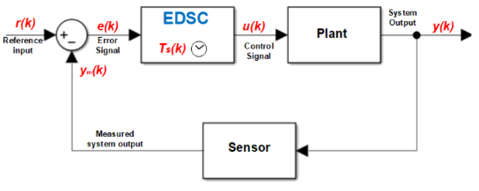
Figure 2.
Variation of Ts and Fs vs. Error.
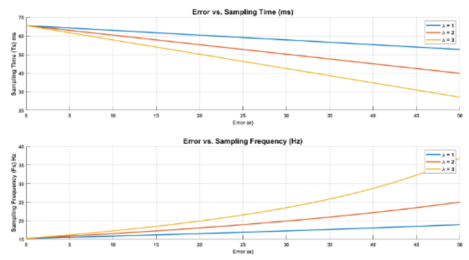
Figure 3.
EDSC block diagram.
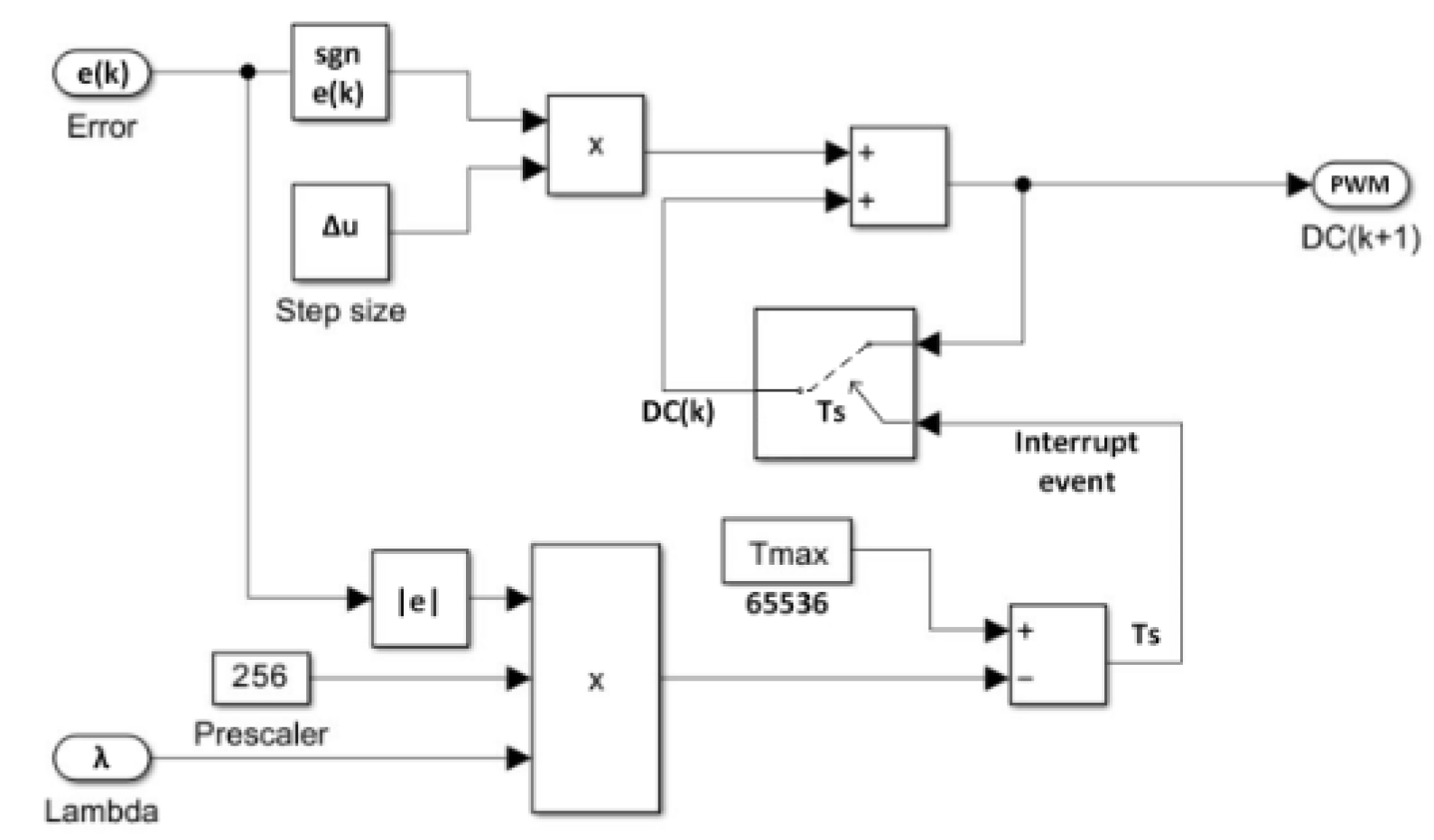
Figure 4.
EDSC simulation result for .
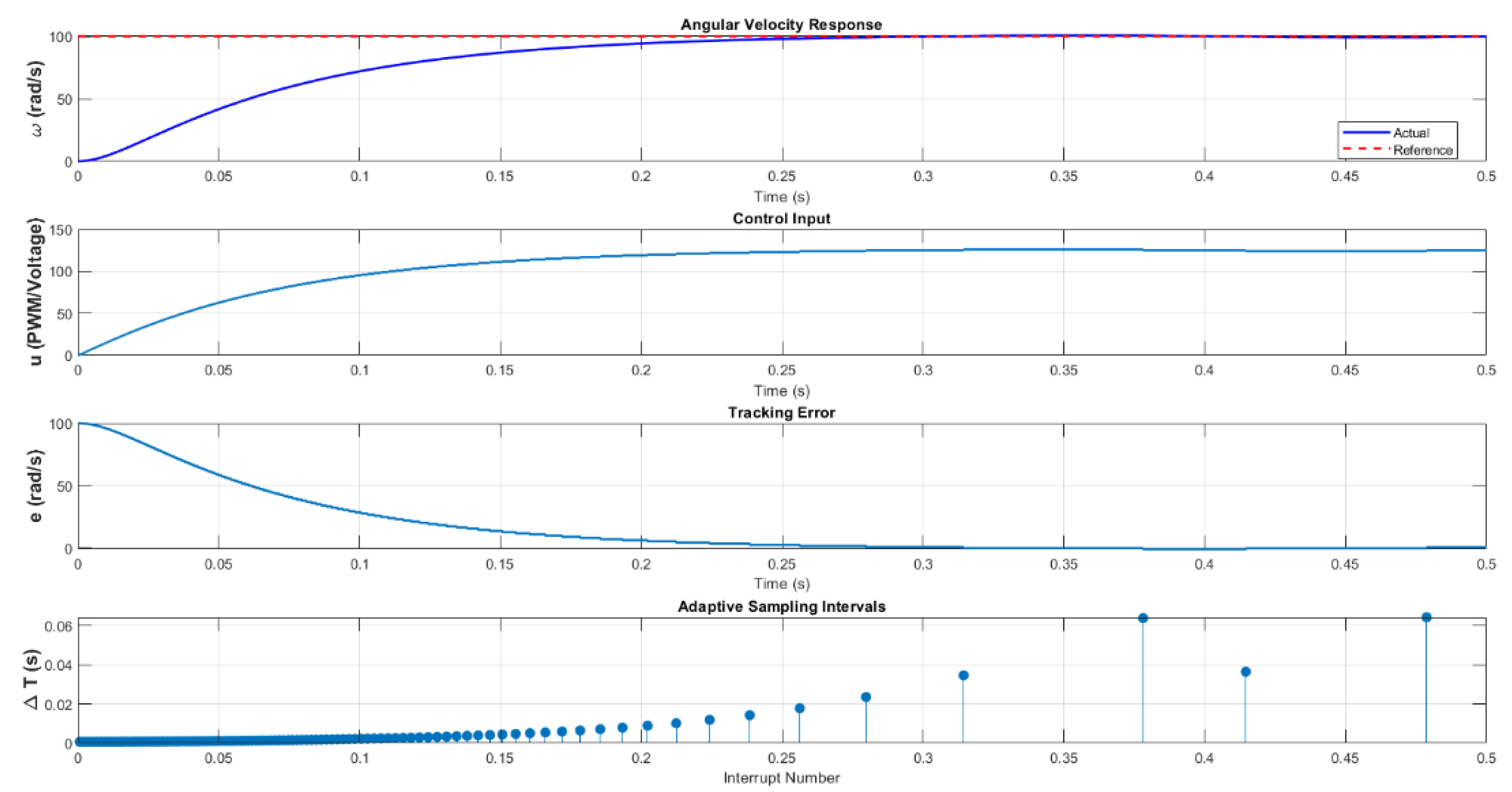
Figure 5.
EDSC simulation result for .
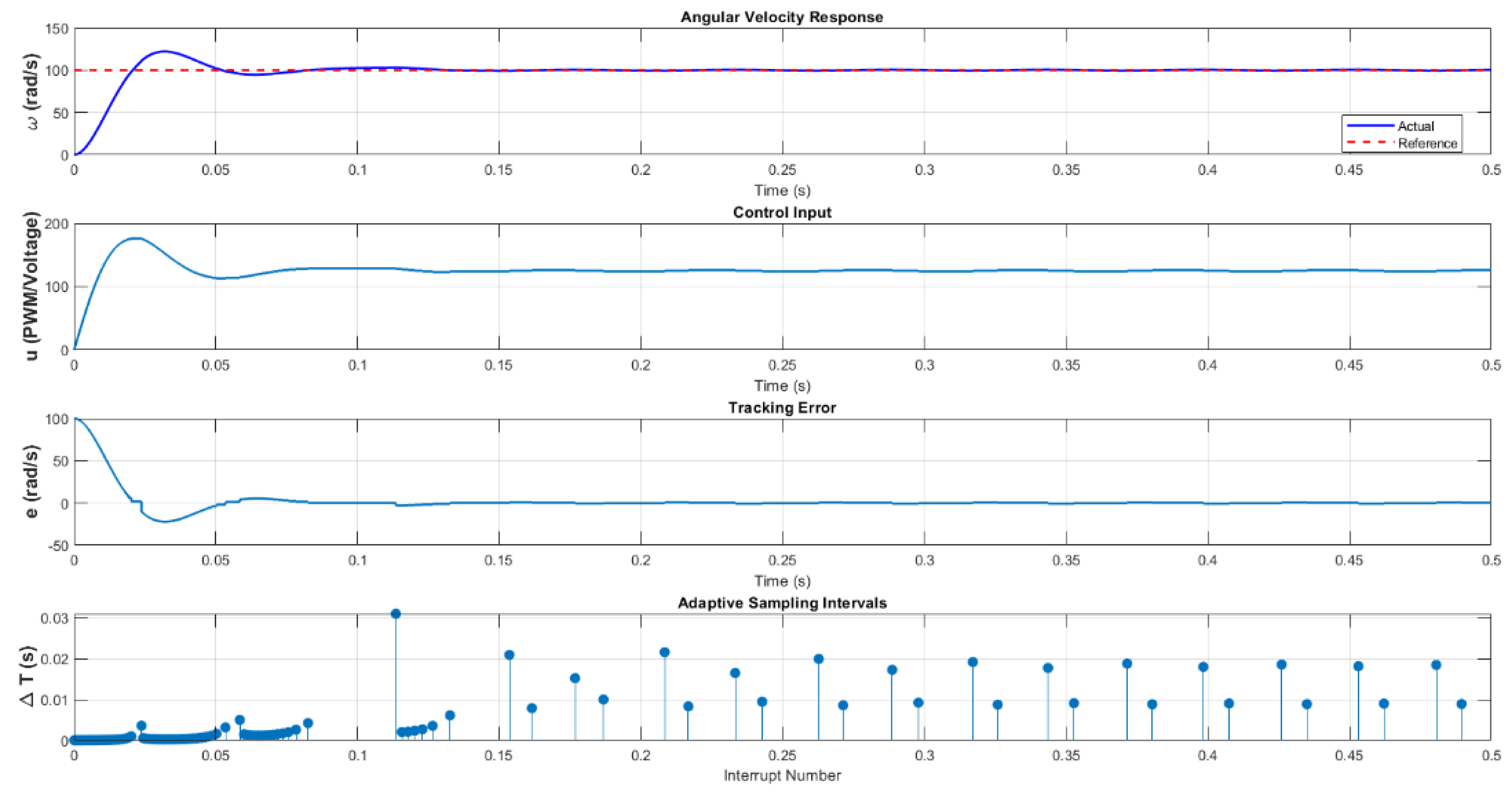
Figure 6.
Lyapunov Function V(e) over time for and .
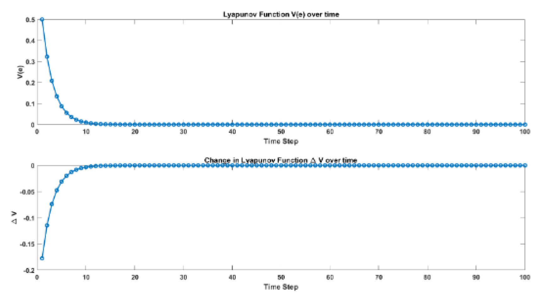
Figure 7.
Timer0 interrupt handler code snippet.
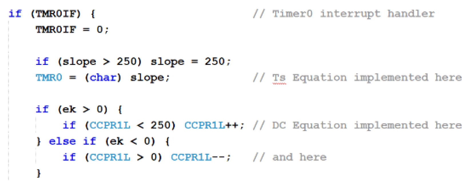
Figure 8.
Main loop code snippet.

Figure 9.
Hardware design setup.
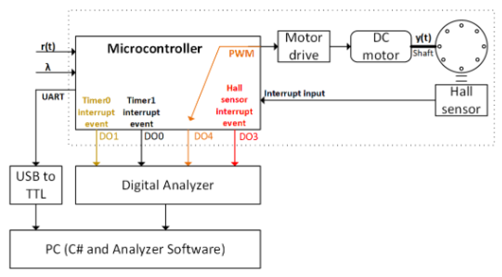
Figure 10.
Response of the motor for .
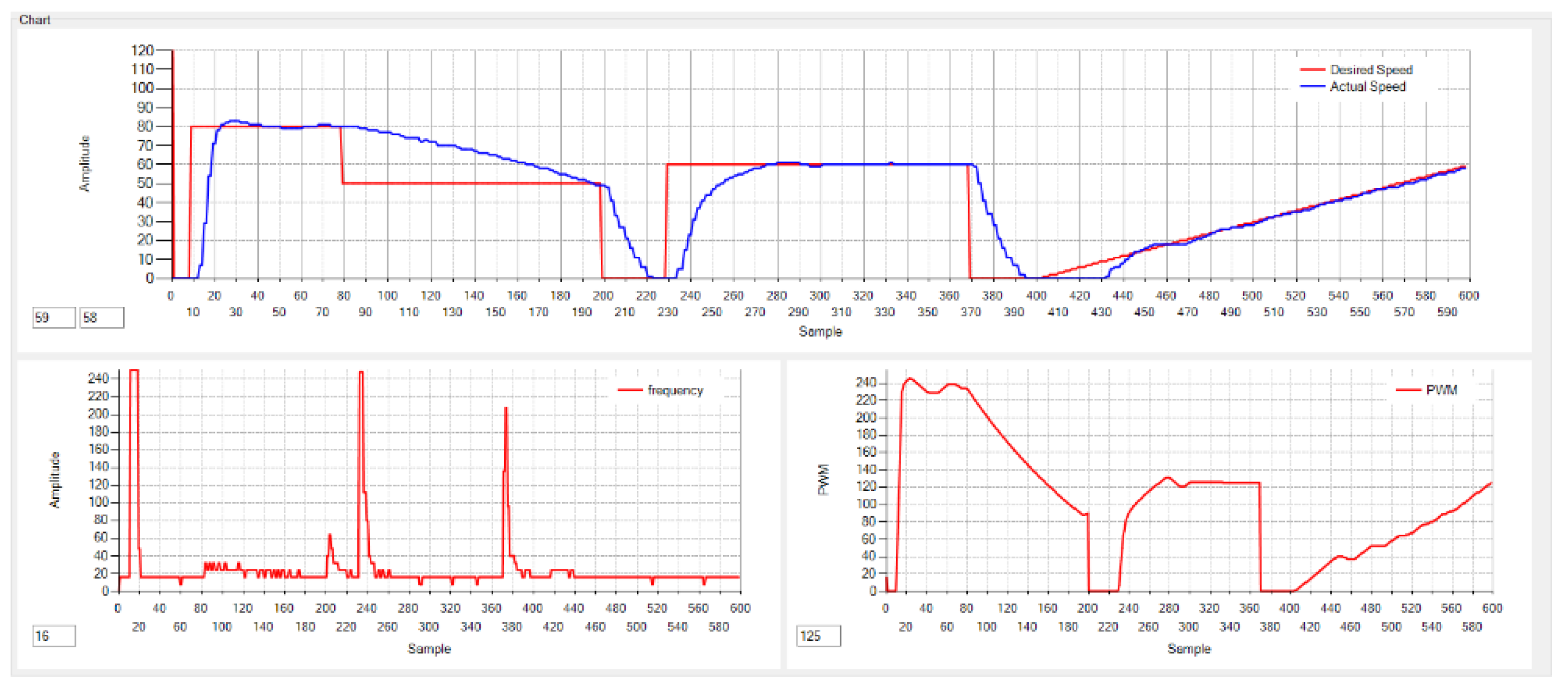
Figure 11.
Response of the motor for .
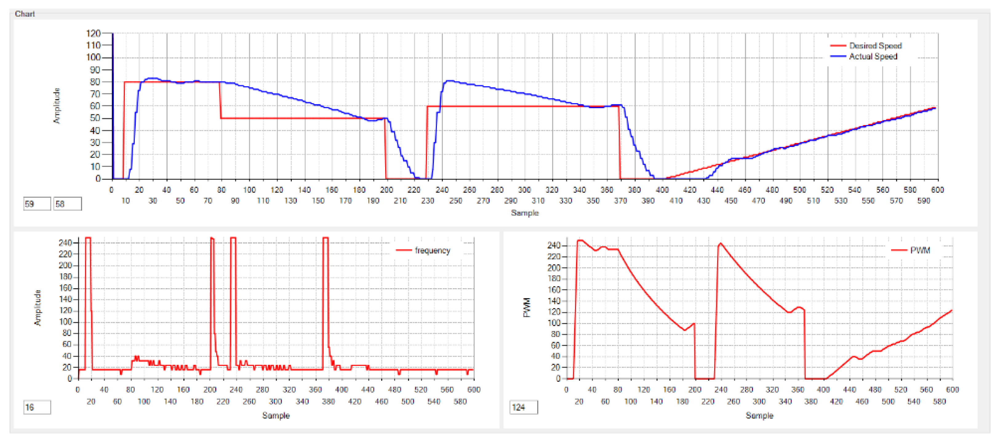
Figure 12.
Response of the motor for .
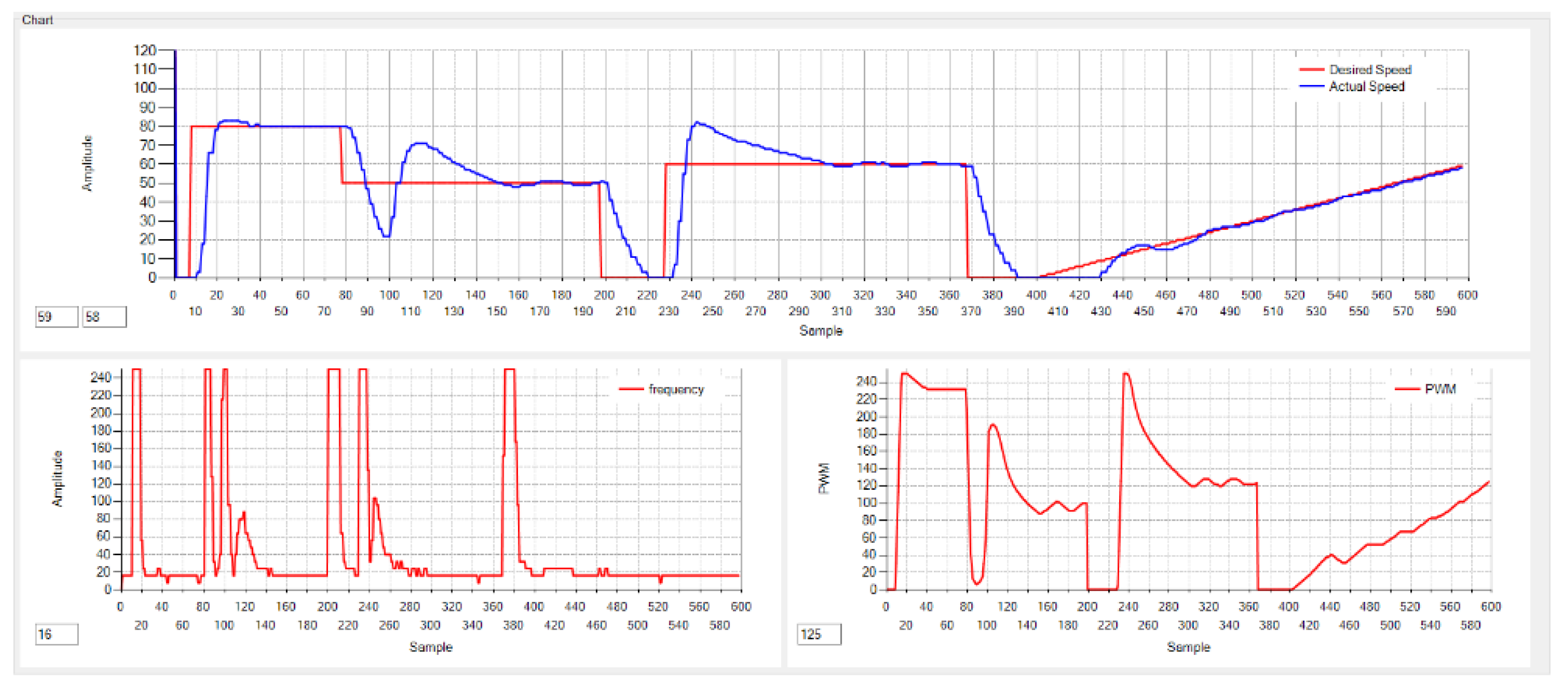
Figure 13.
Logic signals showing interrupt events and the PWM signal, alongside the motor response for over the time interval to s.
Figure 13.
Logic signals showing interrupt events and the PWM signal, alongside the motor response for over the time interval to s.
Disclaimer/Publisher’s Note: The statements, opinions and data contained in all publications are solely those of the individual author(s) and contributor(s) and not of MDPI and/or the editor(s). MDPI and/or the editor(s) disclaim responsibility for any injury to people or property resulting from any ideas, methods, instructions or products referred to in the content. |
© 2025 by the authors. Licensee MDPI, Basel, Switzerland. This article is an open access article distributed under the terms and conditions of the Creative Commons Attribution (CC BY) license (http://creativecommons.org/licenses/by/4.0/).
Copyright: This open access article is published under a Creative Commons CC BY 4.0 license, which permit the free download, distribution, and reuse, provided that the author and preprint are cited in any reuse.


