Submitted:
29 April 2025
Posted:
30 April 2025
You are already at the latest version
Abstract
Accurate clustering of buildings is a prerequisite for map generalization in densely populated urban data. Edge state buildings at the edge of building groups, identified through human-eye recognition, may serve as boundary constraints for clustering. This paper proposes the use of seven Gestalt factors to distinguish edge state buildings from other buildings. Employing the DGI model to produce high-quality node embeddings, optimize the mutual information between the local node representation and the global summary vector. We then conduct training to identify edge state buildings in the two test datasets using eight feature combinations. This research introduces a modified distance metric called the ‘m_dis’ feature, which is used to describe the closeness between two adjacent buildings. Finally, the clusters of edge and inner state buildings are determined through a constrained graph traversal that is based on the ‘m_dis’ feature. This method is capable of effectively identifying and distinguishing densely distributed building groups in cities, as demonstrated by experimental results. It offers novel concepts for edge state building recognition in dense urban areas, confirms the significance of the LOF factor and the ‘m_dis’ feature, and achieves superior clustering results in comparison to other methods. Additionally, this semi-supervised clustering method (DGI-EIC) has the potential to achieve an ARI index of approximately 0.5.
Keywords:
building groups
; DGI model
; clustering
; edge state building
; modified-distance
1. Introduction
Cartography is an academic field focused on the processes involved in scale reduction for maps. The essence resides in the efficient conveyance of information within limited map space via the abstraction of geometric information. In urban map generalization, the boundary structure and shape pertaining to buildings are both significant and intricate. Owing to the dense arrangement of buildings, they must initially be grouped [1], succeeded by map generation operators such as amalgamation and displacement [2,3,4,5].
Buildings, like complex planar polygons, possess attributes including size, orientation, shape, and distribution density. In the context of building clustering, algorithms must thoroughly ascertain the geometric attributes of the building, along with its distribution density and orientation, and establish constraints that adhere to Gestalt principles (proximity, similarity, closure, continuity) to optimize the clustering result [3,6,7,8].
Some clustering methodologies regard buildings as nodes, with the edge between two adjacent buildings representing the graph edge, thereby converting the clustering issue of buildings into node clustering problems within graphs. Examples include clustering based on multi-layer graphs [9,10,11] and local or global edge cut-off based on the density of local Gestalt features and variance values [12,13,14].
Building groups frequently exhibit regular geometric, semantic, and structural features [15]. Research indicates that vertical and linear patterns significantly improve the aggregation effect of buildings [16]. We deduce that the visual characteristics of buildings, including elongated forms, uneven surrounding density distribution, and C-shaped, L-shaped, or U-shaped buildings [17], can be classified as boundary structures of clusters.
The distribution of buildings is irregular, and the reasonable expression of many Gestalt rules [18,19], as well as the automatic identification of edge state buildings, presents several challenges. Certain density-based clustering techniques examine the distribution density of buildings and the delineation of grouping boundaries [20,21,22,23,24,25].
Neural networks is the technique for information transformation that effectively represents the multidimensional attributes of buildings. Self-Organizing-Map (SOM) is employed to identify the contours and boundaries of building clusters [2]. The graph convolutional network (GCN) enhances the contour feature analysis of building clusters by categorizing buildings into three states: edge, inner, and free [26]. By integrating Fourier transform with GCN technology, building features are converted into the embedding space and subsequently grouped utilizing the k-means method [27]. These investigations demonstrate that neural networks serve as a potent deformation mechanism capable of nonlinearly transforming Gestalt factors of intricate building structures, thus producing readily identifiable building structures in embedded space.
Graph Convolutional Networks (GCN) is a robust semi-supervised classification method for graph-structured data [28]. Graphical convolutional networks (GCNs) can encapsulate the characteristics of buildings and their edges (including distances and comparisons of neighboring structures) via local graph convolution operations to derive intricate Gestalt features within groups of buildings.
At present, there is a significant scarcity of research on the characteristics of edge state buildings, with the available research primarily focusing on three indicators: Local statistics (CV value) [24], which is the ratio of the standard deviation to the mean of the local arrangement of the Gestalt feature. The local coordinate deviation, which can be calculated by the center coordinate of the smallest bounding rectangle (SBR) of the central building node and its neighbors [26]. The CDC method measures the local centrality by calculating the directional uniformity of KNNs [29] to distinguish internal and boundary points [30].
This work examines the Deep Graph Infomax model (abbreviated as DGI [31], a kind of Graph Comparative Learning Model) to delineate the edge state building inside the building group and to obtain the building clusters. The binary classification of buildings as either edge state or inner state is accomplished by augmenting the mutual information between local node embeddings and global summary vectors. This approach may differentiate between edge state and inner state buildings inside building clusters on densely populated metropolitan maps. This approach is referred to as the Edge state and Inner state Clustering method with the DGI model, designated as DGI-EIC.
The subsequent sections of this article are structured as follows. Section 2 encompasses the edge state features of the building, the interpretation of the DGI model, and an explanation of graph traversal based on the m_dis constraints. Section 3 displays three experiments. The initial experiment involves the labeling of the edge state buildings of the training dataset through the use of automated rules and manual modifications. The second experiment aims to illustrate the binary classification results of the DGI model under eight feature combination training conditions. The third experiment involves a comparison of the clustering results of the DGI-EIC method in this paper with those of the CDC [30] and Multi-Graph-Partition methods (abbreviated as MGP) [11]. Section 4 is a discussion.
2. Materials and Methods
We maintain that buildings can be classified into two categories: edge state buildings and inner state buildings. Edge state buildings are buildings situated on the outer perimeter of the building group. The P-building in Figure 1 is an example of an edge state building that is typically conspicuous due to the stark contrast in visual features between the buildings on either side. The slender, concave shapes of these structures (C-typed, U-typed, L-typed) and the uneven density distribution surrounding them are frequently used to identify them. The appearance of the building group is typically defined by the presence of edge state buildings surrounding inner state buildings in clustering results. The distribution density, distance, and shape of the inner state buildings are in high balance in relation to the surrounding buildings, as they are situated in the interior area of the cluster. The visual characteristics of the inner state buildings are more consistent than those of the edge state buildings.
The identification of edge state building is the primary focus of this study in order to accomplish effective building clustering. The following features are used to identify edge state buildings: directionality, distribution density, and geometric shape (such as C-shaped, L-shaped, or U-shaped). These characteristics can assist in determining whether the building constitutes a visual boundary. The inner state buildings are subsequently categorized into the corresponding cluster by examining the spatial relationship between the inner state buildings and the adjacent edge state buildings. This approach guarantees the constraints of edge state buildings while simultaneously optimizing the clustering attribution of inner state buildings, thereby concluding the overall clustering assignment. The context of edge state and inner state buildings is illustrated in Figure 1:
Polygons marked with a red stroke indicate edge state buildings, while those marked with a blue stroke indicate inner state, as illustrated in Figure 1. The buildings are identified by letters, with the building number P designated as an edge state building. A building group is formed by the inner state buildings A, B, H, and I, which are surrounded by the edge state buildings C, G, and P, which form a very obvious L-shaped boundary constraint. Buildings D and F are evidently not included in any sub-cluster, while buildings E and J constitute a local sub-cluster.
It is important to note that the classification method employed in this study only categorizes buildings into two types: edge state buildings and inner state buildings. It does not include the "free state buildings" that have been discussed in previous studies [26]. The following section will provide a comprehensive description of the identification characteristics of edge state buildings.
2.1. Descriptive Methods for Edge State Building Features
The building and its association relationship can be represented as graph structural data in the study of building clustering. Nodes represent buildings, and edges represent spatial associations between buildings. Suppose we have a graph G=(V,E), where V and E are the sets of nodes and edges, respectively, and the number of nodes is N. The node feature matrix is formed by the representation of the feature of each node i∈V as , where F is the number of features and N is the number of nodes. The adjacency matrix represents the edge structure information of each building node in the graph. If , it indicates that there is an edge between building node i and building node j; otherwise, it is 0. The Voronoi diagram units constructed at the encrypted boundary points of the building are combined to create the polygonal Voronoi diagram division of buildings [32], which can be observed in Figure 4 (a). The graph structure is formed by establishing the incident edges of two adjacent buildings based on the proximity relationship of the Voronoi diagram polygon.
2.1.1. Expand the K-NN Neighborhoods in Graph
The Euclidean distance between each building and its k nearest neighbor elements is determined by the conventional K-NN procedure. This neighborhood range expression simplifies the process of obtaining spherical neighborhood results. The natural adjacency relationship between the margins of buildings facilitates the construction of neighborhoods. This paper employs the shortest path algorithm and graph structure to define K-NN neighborhoods in the graph structure space, thereby obtaining K-NN expressions that are appropriate for constructing distribution characteristics. The length of the associated edges is used to quantify the distance between buildings. The is defined as the distance between buildings v and u, taking into account their volume and size:
In formula 1, The path distance between node v and node u is denoted by d(v,u), which is calculated using the classic Dijkstra algorithm [33]. The mean radii of the buildings represented by node v and node u are r(v) and r(u), respectively [34]. The spatial volume of a building is more significant as its radius increases, which is then manipulated as a closer relationship in the distance calculation. The constant "0" in the formula is employed to prevent issues with negative value calculations. The volume characteristics of the building can be effectively taken into account by this correction distance. Larger buildings are more likely to be considered in close proximity at the same path distance.
This paper further defines the neighborhood relationship of a building, selects a building node p as the starting point, calculates its shortest path distance from other nodes based on the graph structure, and arranges the path distances of all other nodes. The k-neighborhood collection of node p is composed of the first node to the k-th node of the sorting result of path distance, arranged in order of distance from small to large. The path distance between node u1 and node p is the minimum, and it is denoted as d1(p), as illustrated in Figure 2.
The distances of the nine points to point P in Figure 2 are as follows:. The following two definitions are straightforward to comprehend, as indicated by Figure 2.
Definition 1 K-distance from building P
The k-distance is the distance between the k-th nearest neighbor and point P. For node P, its K-distance is defined as formula 2 :
Among them, is the i-th neighbor sorted from small to large by the distance from point to point P. If the number of neighbors is less than k, then is the farthest distance among all neighbors at point P.
Definition 2 K-NN neighborhood of building P
A set of K-NN neighbors of node p is defined as a neighborhood with a distance of no more than .
where is the number of the i-th neighbor sorted by distance.
2.1.2. The LOF Characteristic of the Building [21]
The formula 4 defines the local reachable density for building P, which is the inverse of the average reachability distance based on the K-NN neighborhood of P.
|kn(P)| is the number of elements in the K-NN neighborhood of building P in formula 4 and is the distance between point P and point in the K-NN neighborhood of point P. The LOF feature of point P is the average of the ratio of the local reachable density of each point in point P’s K-NN neighborhood to the local reachable density of point P. This feature represents the density of the local distribution of data, which is defined as . The formula is as follows:
In formula 5, |kn(P)| is the number of features in the K-NN neighborhood of point P. is the local reachable density of point in the K-NN neighborhood of point P.
2.1.3. The Center_Devia and First_Neighbor_avg_r Features of Buildings
Figure 3 illustrates the points that constitute the first-order neighborhood of point P, which are points A, B, C, D, E, F, and G, respectively. A first-order neighborhood polygon of point P is formed by connecting them in sequence. Point R is the geometric centroid of this polygon. The center_devia feature of the P point is the length of vector. The first_neighbor_avg_r feature is the average distance of the center of the polygon and each vertex of the polygon. As illustrated in Figure 3, the first_neighbor_avg_r is the average of the lengths of PA, PB, PC, PD, PE, PF, and PG.
2.1.4. The Density and vo_to_b_Length Characters of the Building
To achieve the division of building space units, the building boundaries are initially encrypted. Subsequently, the Voronoi graph polygon is generated using the encrypted nodes. The Voronoi polygons generated by nodes within the same building are merged, and the Voronoi graph division results of the building are subsequently obtained [32]. Figure 4 illustrates the buildings and their corresponding Voronoi diagram unit.
Figure 4.
(a) The encrypted points and their Voronoi diagrams; (b) The buildings and Voronoi diagrams.
Figure 4.
(a) The encrypted points and their Voronoi diagrams; (b) The buildings and Voronoi diagrams.

In Figure 4 (b), the blue stroke area represents the Voronoi diagram unit where the building is located. The starting point of the red arrow line is the center of the Voronoi diagram unit, and the end point is the center of the building. This red arrow indicates the position where the building deviates from the center of the Voronoi graph unit, which can express the distribution of the building. The area of a building divided by the area of the Vornoi diagram unit is the density feature [34]
2.1.5. The m_dis of Two Adjacent Buildings and the m_dis_cv Character of a Building
We propose a modified distance (abbreviated as m_dis) between two adjacent buildings and generate the coefficient of variation for modified distances (abbreviated as m_dis_cv) of a building. There are detailed descriptions of the modified distance in Figure 5.
In Figure 5, A is a polygon, and B, C, D, and E are four polygons surrounding A. The shortest distances between A and B, C, D, and E are denoted as dab, dac, dad, and dae, and the inner widths of A, B, C, D, and E are ha, hb, hc, hd, and he. Among them, the internal widths of B, C, and E are equal, while the internal width of D is larger.
Figure 5 shows that polygons with the same inner width (like polygons B and E) are more likely to be linked to A by shorter distances. Since B and A are closer, they are more likely to be in the same cluster. Similar classifications applied to polygons with larger inner widths. Because D has a wider inner width, D and A are more associated despite C having the same distance to A. This correlation defines the modified distance for every two nearby buildings, and the computation formula is as follows:
In the formula, A and i represent the buildings at both ends of their incident edge, d(A,i) is the closest distance between buildings A and i, and and are the inner widths of buildings A and i. For complex polygons, this inner width is difficult to calculate. In this study, the mean radius [34] is used to represent the inner width. The mean radius means the average distance from each vertex of the building to its centroid [35].
For a building, all the m_dis of its incident edges constitute a numerical set, characterized by mean and standard deviation. The coefficient of variation of these m_dis can be shown as formula 7:
In formula 7, is the m_dis of the edge of the i-th building adjacent to A building, std is the standard deviation, and mean is the average. The larger this value, the more deviated the distribution of m_dis features, and the more likely the A building is an edge state building.
In conclusion. Table 1 illustrates the seven characteristics that determine whether the building is an edge state building. If it is an edge state building, we assign it an attribute termed whether_ edge = 1, else the whether_edge attribute is 0.
2.2. The Node Representation Learning Based on DGI Model
The DGI model offers a robust node-embedded representation learning technique for graph-structured data by maximizing local-global mutual information. It excels in numerous tasks, particularly in inductive learning that surpasses conventional unsupervised methods [31]. This paper employs the DGI model to determine edge state buildings and conducts a binary classification (edge state or inner state) of buildings graph from the training set to the test set.
To extract the high-level features of the building, we employ a graph convolutional neural network as an encoder to map building node features and graph structure into node embedding space, thereby obtaining the higher-level representation of the node , where represents the embedding of node i and denotes the embedding dimension. The method of generating node embeddings can be articulated as follows:
In formula 8, the is a graph convolution encoder that generates embeddings by aggregating the immediate neighbors of each node. These embeddings encapsulate the characteristics of a specific building while also integrating its contextual information within the graph. The generated node embedding hi encompasses a "subgraph" of a graph centered on node i, rather than exclusively the node itself. It is termed "subgraph representations".
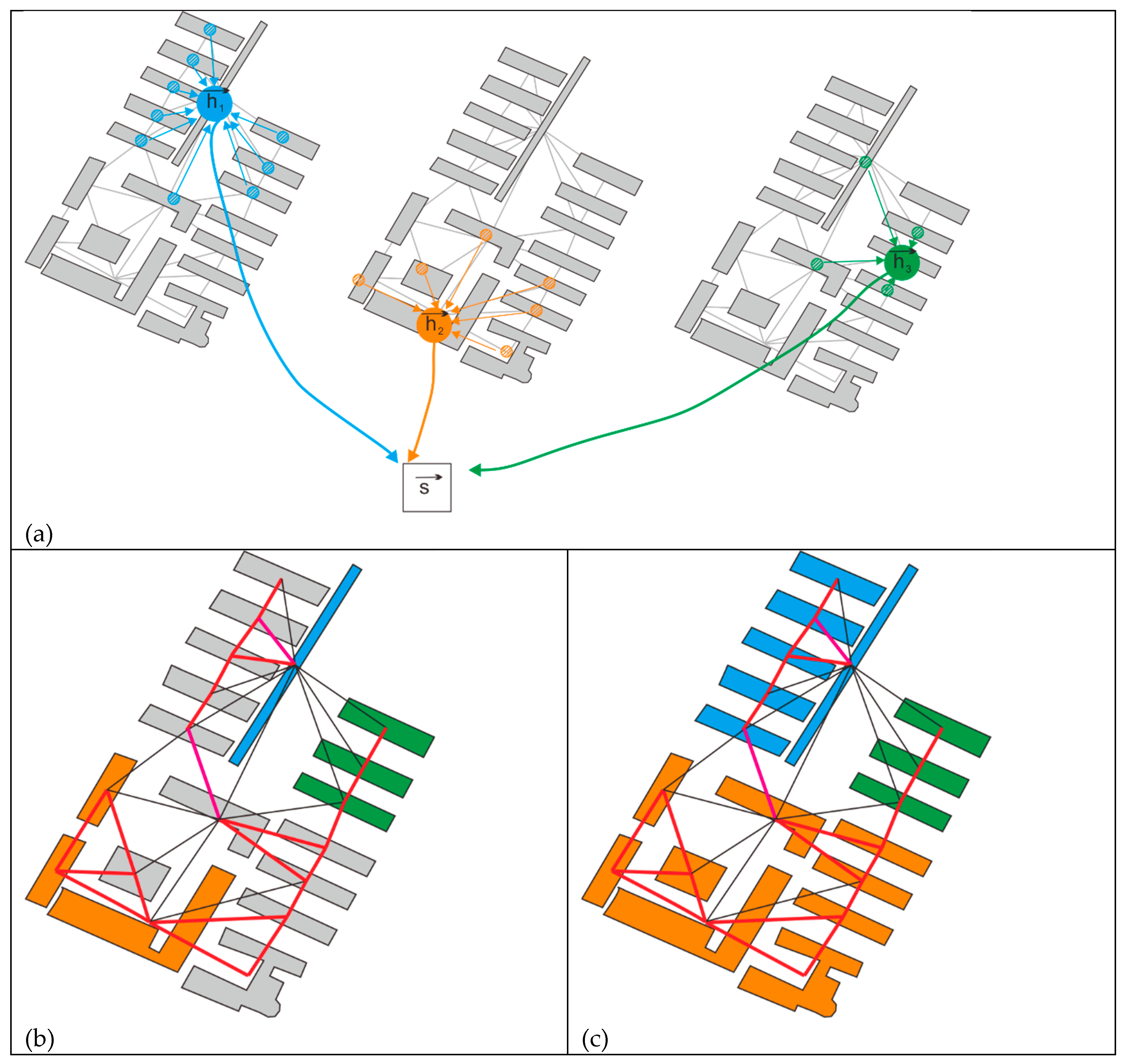
We utilize an unsupervised learning approach aimed at optimizing local-global mutual information to produce node embeddings that encapsulate both global and local information. The objective of the DGI model is to augment the mutual information between node embeddings and the graph-level summary vectors . Each node's embedding signifies its distinct characteristics while ensuring coherence with the comprehensive information of the graph. The global graph summary vector is derived by aggregating all node embeddings, reflecting the overall semantic content of the graph. The graph convolution mechanism transforms the characteristics of building nodes into vectors . Subsequently, the local embedding vectors of every building are combined to create a summary vector . Figure 7 (a) illustrates the process of building node features transformation and aggregation.
We train a discriminator by producing positive samples (node embeddings and global summaries from entire graphs) and negative samples (node embeddings and global summaries from altered graphs), therefore enabling node embeddings to encapsulate more nuanced representations.
We first consolidate all nodes within H into a comprehensive graph-level summary vector through a readout function , represented as , where the R function in this article aggregates nodes into a global graph summary. This function implements the average output of each dimension of the node. The function is utilized to extract the global semantic information of the entire graph. This global overview delineates the overarching attributes of the building graph. To enable the comparison of local and global information, we generate pairs of positive and negative samples, positive samples are , while negative samples are .
The positive sample comprises the node embedding and the global graph summary of the original graph, encapsulating both local and global information within the same graph. The negative sample graph is generated by perturbing the original graph, for instance, by randomly modifying node features or edges, and the node embedding is derived from it. The negative samples are provided by pairing the summary from with patch representations of an alternative graph. This is shown in Figure 6.
The DGI model developed a discriminator to differentiate between positive sample pairs (from the original graph) and negative sample pairs (from an alternative graph). The discriminator enhances node embedding through comparison learning, enabling it to discern the relationship between local and global information. The objective function for optimization is a type of binary cross-entropy loss [31], which is in formula 9:
In formula 9, N is the number of positive samples, and M is the number of negative samples. By maximizing the scores of positive sample pairs while minimizing the scores of negative sample pairs, the DGI model is able to learn high-quality node embeddings. The structure of the DGI model is shown in Figure 6:
In Figure 6, is the original node feature , is the high-dimensional embedding representation of the node, is the perturbation operation of the node feature, and the is the operation to generate node embedding, is the readout function, is the global graph summary vector, and is the discriminator.
2.3. The Traverse of Building Graph
After segmenting the edge state buildings from the building graph, the constraints derived from m_dis characteristics are examined to provide the clustering results of the building graph. Initially, the natural breakpoint approach [38] is employed to categorize the m_dis features into four levels, with the third-level m_dis feature value designated as the separation threshold. When the m_dis value is below the third level, it signifies a reduced m_dis feature between the two buildings, suggesting proximity and potential categorization within the same group; conversely, a higher m_dis value indicates an increased visual distance, implying they may belong to distinct categories.
The buildings in the graph structure are traversed to create the initial cluster, after which the buildings of the established clusters are removed from the total building set. A subsequent traversal is conducted to generate the second cluster, and this process continues until all edge state buildings have been organized into their respective clusters. The design of the specific traversal algorithm is illustrated in the pseudo-code:
| Algorithm BFS with KY Value Limit for Graph Traversal | |
| 1 | Input: Graph G=(V,E) (where V represents buildings and E represents edges), starting building Vstart , threshold m_dis_limit |
| 2 | Initialize: visited: an empty set to store visited buildings. queue: a list initialized withVstart. traversal_result: an empty list to store the result of BFS traversal. |
| 3 | While queue is not empty do: |
| 4 | Pop the first building Vcurrent from queue. |
| 5 | If Vcurrent ∉ visited and G[Vcurrent].we=1: |
| 6 | Add Vcurrent to visited. |
| 7 | Append Vcurrent to traversal_result. |
| 8 | For each neighbor Vneighbor of Vcurrent: |
| 9 | If Vneighbor∉ visited: |
| 10 | Retrieve edge_data for (Vcurrent,Vneighbor). |
| 11 | If edge_data exists and edge_data.m_dis ≤ m_dis_limit |
| 12 | Append Vneighbor to queue |
| 13 | Return: traversal_result. |
In pseudocode, the variable G[Vcurrent].we denotes the whether_edge attribute (described in section 2.1.5) of the current node Vcurrent. A value of 1 signifies that the node is an edge node. In reference to Figure 7, the edges are depicted in black when their m_dis feature value is below the established threshold; conversely, if the m_dis feature value exceeds the threshold, it is represented in red. Upon establishing the boundary structure, categorize the nodes by navigating the graph along the red edge. During the traversal process, in the absence of a red edge on the current side, the accessed edge state buildings are classified into a distinct building group. This procedure persists until all edge state buildings are visited. In the illustration, colored nodes signify edge state buildings, which are designated distinct numbers during traversal to identify their respective clusters; the gray color denotes inner state buildings, with their cluster numbers determined by the cluster numbers of their nearest edge state building.
Figure 7.
(a) The vector is local graph convolution of buildings, and all constitute the summary vector , ; (b) Three edge state building clusters after the traverse; (c) Allocate inner state buildings to clusters based on proximity to adjacent edge state buildings.
Figure 7.
(a) The vector is local graph convolution of buildings, and all constitute the summary vector , ; (b) Three edge state building clusters after the traverse; (c) Allocate inner state buildings to clusters based on proximity to adjacent edge state buildings.
3. Results
This paper's experimental data comprises two city datasets. The Chengdu data originates from the production department, involving semi-automatic map generation (abbreviated as CD data). The Nanchang city data was downloaded from the OpenStreetMap website [39] (abbreviated as NC data). The training dataset originates from the CD dataset, comprising 4,851 buildings, while the test1, test2 datasets are derived from the CD and NC datasets, containing 689 and 1,737 buildings, respectively. The Figure 8 and Table 2 illustrates that the CD data is irregular, exhibiting a predominance of concave shapes. Various shapes of buildings exist, such as C-shaped, U-shaped, Z-shaped, L-shaped, and octopus-shaped structures. The NC data indicates a higher incidence of rectangles, and the orientation of the buildings is relatively consistent.
From Table 2, describing the experimental data, we can see that the Chengdu data (CD) contains more concave polygons and more buildings are not regular rectangles, while the Nanchang data (NC) contains more convex polygons and more regular rectangles.
The subsequent three experiments are as follows: 3.1, semi-automatically identify the edge state buildings in the training dataset; 3.2, employ the DGI model to train the dataset in order to acquire the model parameters. In 3.3, utilize the parameters acquired from model training to perform binary classification of edge state buildings and inner state buildings on test1 and test2 dataset. Utilize the graph traversal method (described in section 2.3) to obtain the clustering results of test1 and test2, and compare these results with the results of the CDC method[30] and MGP method[11].
3.1. Experiment for Semi-Automatically Labeling Edge State Buildings
This subsection pertains to the execution of edge state building delineation. We utilize the Local Outlier Factor (LOF) and the vector length from the Voronoi polygon center to the building center (vo_to_b_length) to develop edge state building labeling. The following are the procedural steps:
3.1.1. Attribute Definition and Grading
The LOF attribute denotes the degree of local outlierness of a building, with elevated values signifying an increased probability of the building being situated at the periphery. Utilizing the natural break method [38], the LOF attribute is categorized into three tiers: low-value range (0.838–0.995), medium-value range (0.995–1.055), and high-value range (1.055–2.000). The vo_to_b_length attribute indicates the vector length from the center of the Voronoi polygon to the center of the building. Greater values reflect a more significant divergence between the Voronoi polygon center and the building center. According to the natural break method, this attribute is also classified into three levels: low-value range (0.02–3.24), medium-value range (3.24–8.70), and high-value range (8.70–115.41).
3.1.2. The Semi-automated Labeling of Edge State Buildings
Initially, employ the subsequent regulations to autonomously identify the edge state buildings:
- When a building's vo_to_b_length value falls within the high-value range (>8.690), it receives the label of an edge state building (whether_edge=1).
- If the vo_to_b_length value falls within the medium-value range (3.236–8.690) and the corresponding LOF value falls within the high-value range (>1.055), it is also labeled as an edge state building (whether_edge=1).
- Buildings that do not satisfy the above conditions are labeled as inner state buildings (whether_edge=0).
Ultimately, a collection of labels that are consistent with the human identification results is obtained by manually modifying a few labels after the edge state building is automatically marked. The training dataset contains 2065 edge state buildings that are automatically labeled according to the rules and 727 edge state buildings that are manually modified, resulting in 2792 edge state buildings in total. Similarly, we added labels of edge state buildings to the test 1 and test 2 datasets to evaluate the results of the DGI model binary classification.
3.2. The DGI Model Training Phase
The DGI model employed in the investigation has an input feature dimension of 7, corresponding to the edge state building features, while the hidden layer dimension is 512, representing the node embeddings extracted through a graph convolutional network (GCN) module via a linear transformation layer. This layer is activated by a nonlinear function (PReLU). Weight initialization uses the Xavier uniform distribution, with bias terms initialized to zero, enhancing the model's stability and training efficiency. The GCN module aggregates neighbor information through the adjacency matrix, improving computational efficiency by performing matrix multiplication during forward propagation. Each node's embedding is determined by the weighted sum of its adjacent nodes' features, processed through the activation function. The global representation, computed as the average of all node embeddings by the global readout module AvgReadout, is subsequently compressed to the range of [0, 1] using the Sigmoid function, producing a summary vector at the full graph level.
The discriminator module distinguishes the global-local alignment relationship between positive samples (real graph) and negative samples (alternative graph) through contrastive learning tasks. It uses a bilinear layer to calculate the relationship score between the global representation and the node embedding, generating the final learning vector by concatenating the score vectors of positive and negative samples.
We use a logistic regression classifier to binary classify the final learning vectors generated by the DGI model. The input is the embedding vector of the node, with the same dimension as the embedding vector, and the output is a probability distribution indicating whether the node is an edge state or inner state node, with a dimension of 2. The Adam optimizer is employed with a learning rate of 0.01 and weight decay set to 0 to avoid overfitting, training the first 100 samples of the embedding vector. The labels during training are randomly generated.
During training, we calculate the logits (unnormalized probability) output by the classifier, evaluate the cross-entropy loss between the logits and the real label using the cross-entropy loss function [31], and perform backpropagation to update the classifier parameters. After training, the classifier switches to evaluation mode, inferring the embedding vectors of all nodes and processing the logits output by the model through a maximum value index operation to obtain the final binary classification result (edge state or inner state).
We developed training protocols for eight feature combinations to assess their impact on binary classification tasks involving edge state buildings versus inner state buildings. These combinations range from subsets missing a single characteristic to a comprehensive set that includes all seven features, with the goal of evaluating the effect of each feature or group of features on classification performance. The specific combinations are in Table 3:
In each training session, the scales of train, val, and test are identical, accounting for 60%, 20%, and 20% of the total. In order to prevent training from collapsing into overfitting, we implement early stopping by setting a variable named cnt_wait. Whether the current loss is less than the highest loss previously recorded will be verified by the code, cnt_wait will be increased by 1 if the current loss does not improve. The early stopping mechanism will be activated, and the training will be terminated when cnt_wait reaches the predetermined patience value. This suggests that it is necessary to discontinue training in order to prevent overfitting if the loss does not progress after multiple training cycles. In Figure 9, the training loss is illustrated:
The training of each feature combination requires 5 minutes (exclusively on CPU), resulting in a cumulative training duration of 40 minutes for the 8 models (on CPU). Among the combinations, the feature set (1, 2, 3, 4, 5, 7) results in the quickest training termination, concluding in 114 steps. This indicates that the absence of the first_neighbor_avg_r feature facilitates the most rapid convergence of the training process. When utilizing the feature combination (1, 2, 3, 5, 6, 7), the training progresses at the slowest rate, concluding in 233 steps. This implies that when the vo_to_b_length feature is absent, it necessitates additional iterations in the learning process to identify the optimal solution. So, The average radius of a building's first-order neighborhood polygon little influences the determination of its status as an edge state building, while the vector length from the center of the Voronoi diagram unit corresponding to the building’s center, this character significantly influences the determination of whether the building qualifies as an edge state building.
The blue dotted line in Figure 9 represents the negative sample score during training of feature combinations (1,2,3,4,5,6,7), while the yellow dotted line represents the positive sample score during training of feature combinations (1,2,3,4,5,6,7). The average positive sample score of each node embedding is 0.5. The average positive sample score progressively increases as the training commences, ultimately reaching 0.63. The average negative sample score decreases steadily until it reaches 0.34. Positive and negative sample scores are clearly distinguished. The node embedding and the global summary are more correlated, and the mutual information is maximized, as the positive sample score increases. The global summary can suppress noise interference by disregarding the node embedding after the perturbation, as evidenced by a decreased negative sample score. The negative sample score's ideal value is not close to the ideal value of 0, and the average value of the positive sample score in our study is not close to the ideal value of 1. This suggests that the research conducted in this article has the potential for development.
This work employs evaluation metrics for classification results, namely Precision, Recall, and F1-score, to assess the binary classification outcomes of edge state buildings and inner state buildings. The subsequent formula illustrates:
In formulas 10, 11, and 12, TP (true positive) is the count of samples anticipated as positive that are indeed positive. FP (false positive) is the quantity of samples erroneously forecasted as positive while being negative. FN (false negative) is the quantity of samples anticipated as negative that are, in fact, positive. The binary classification outcomes for edge state buildings and inner state buildings, under various combinations of training characteristics, are illustrated in the Figure 10 below:
In Figure 10, the horizontal axis denotes the combination of training features, comprising eight distinct categories. Each combination of features is linked to a model training, labeled as Model 1 to Model 8, while the vertical axis shows the evaluation metrics for binary classification, which are precision, recall, and F1-score. Based on the three measures, Model 8 performed the best, indicating that training buildings requires using all seven features together to improve results.
The indicators for the outcomes of No. 1 training are evidently poor, indicating that m_dis_cv is a significant characteristic when delineating edge state buildings, as it reflects the distribution irregularity surrounding the building, and this parameter is a statistical measure. The m_dis feature (refer to section 2.1.5), which quantifies the spacing and volume of a building, is a distinctive element introduced in this article. The outcomes of training sessions No. 2 to 5 exhibit a significant disparity in precision and recall metrics, with the recall parameters being elevated. The elevated recall parameters suggest the model can identify most positive samples, but the prediction is low and may generate more false positives, implying that the absence of any one of the features: first_neighbor_avg_r, center_devia, vo_to_b_length, or density—will affect the training of edge state buildings. The recall parameter of the sixth training is the lowest, indicating a significant number of edge state buildings are unrecognized. Additionally, the F1-score is the lowest, suggesting that the LOF value is a crucial attribute for detecting edge state buildings, corroborating prior research findings [23]. The poor recall parameter of the seventh training indicates that concavity is a significant characteristic in assessing edge state buildings. Manual visual inspection revealed that a greater number of edge state buildings are configured in L-shaped, C-shaped, and U-shaped forms.
In evaluating the entire perspective of the three indications of the eight feature combination, it is advisable to consider all these seven indicators while assessing edge state buildings. The binary categorization outcomes for edge state buildings and inner state buildings are illustrated in Figure 11:
We employ the parameters derived from the DGI model training result to differentiate between edge state buildings and inner state buildings. Figure 11 (a) indicates that both the training set and the test1 dataset comprise Chengdu data generated by the same department. Consequently, the utilization of training model parameters yields superior results on the test1 dataset, whereas the migration of training set parameters to the test2 dataset results in suboptimal performance. The data morphology, distribution density rules, and other characteristics of the test2 data set markedly differ from those of the test1 data set.
3.3. Clustering Comparison Experiment
The DGI-EIC results were obtained using graph traversal of the m_dis feature value constraints on the edge state and inner state buildings from section 3.2. The clustering results can better describe the building's geometric arrangement's density properties and match human perception using graph traversal methods and m_dis feature constraints.
The DGI-EIC approach was examined and assessed alongside the CDC method [30] and the MGP method [11]. The CDC method utilizes only the x-coordinate, y-coordinate of the building's center point, area, and average distance [34] attributes as input, whereas the MGP method assigns weights to the four Gestalt properties of the edges connecting buildings based on the coefficients (0.6, 0.05, 0.3, 0.05) specified in the original text. Figure 12 below illustrates the comparison of clustering results:
Choose the eight local regions A, B, C, D, E, F, G, and H from the test 1 and test 2 datasets for amplification, as seen in Figure 13 and Figure 14 below, to further demonstrate the enhancements of the DGI-EIC approach. Figure 13 presents a slightly amplified segment of the test 1 data set, whereby areas A and the DGI-EIC method indicate that the cluster of E-type in the upper left corner exhibits superior recognition efficacy (highlighted as the red region). The form of this cluster, resembling a rectangle, aligns with the cognitive findings related to human vision; yet, neither the CDC technique nor the MGP approach can discern the E-type cluster. The region of Figure B reveals that the green cluster found by the DGI-EIC approach also encompasses the pink cluster, suggesting that the method remains incomplete. Nonetheless, the pink cluster detected by the CDC technique is illogical, contradicting human visual identification results, and the green area identified by the MGP method is similarly nonsensical. The substantial horizontal Gestalt alignment characteristic between the two buildings in the cross-domain roadway is erroneously classified as a cluster. In region C, the orange cluster delineated by the DGI-EIC approach is excessively large, revealing a flaw in the clustering outcomes. The CDC algorithm demonstrates superior recognition outcomes (shown by the green area). The MGP technique also suffers from unreasonably large cluster areas. In area D, the DGI-EIC approach accurately identifies the cluster of buildings on either side of the roadway, whereas the CDC method erroneously categorizes structures on both sides as a single category, a flaw also present in the MGP method.
The 4 locally enlarged areas of test 2 are in Figure 14 below. For area E, the sub-clusters of buildings divided by streets can be identified by the DGI-EIC method, but the CDC method cannot be identified (green cluster area). For area F, the results of the DGI-EIC method are too broken, while the results of MGP recognition are better. The results identified by the CDC method have cluster boundary crossing. For the G area, the DGI-EIC method has better identification results, while the CDC method has wrong identification results (green buildings should be the same as blue buildings), and the yellow clusters identified by MGP are wrong results. For the H region, the results of the DGI-EIC method do not have the phenomenon of crossing the boundaries of the clusters, while the results of the CDC and MGP methods all have the problem of crossing the boundaries of the clusters.
This is because the test2 data set is a kind of data with uneven density distribution. The key in the MGP algorithm is the weighting coefficient for gestalt factor and distance. For local areas with different densities, the feature weighting and parameters of the associated edges are the same, so some local areas cannot be distinguished. Even if the node exchange mechanism is added, the first step of graph node merge is wrong, which is hard to correct in the subsequent node exchange.
If the building characteristics exceed three, the CDC algorithm determines the angle variance of the building's k-nn neighbors, which is a high-dimensional space. Ordinary individuals are incapable of comprehending the distribution variance of this high-dimensional space. Thus, CDC clustering cannot approximate human eye recognition.
The clustering results of Test 1 and Test 2 data sets are evaluated using these indexes: silhouette coefficient, Davies-Bouldin index, Calinski-Harabasz index, and ARI [40]. The results of index statistics are as Table 4 shows:
Table 4's index analysis indicates that the Silhouette Coefficient for the DGI-EIC method, the CDC method, and the MGP method exhibited subpar performance. The assessment of the Silhouette Coefficient primarily relies on the four attributes of x-coordinate, y-coordinate of building’s center, area, and average distance, whereas the differentiation and internal cohesion among the building clusters encompass more intricate Gestalt characteristics. Consequently, the aforementioned three evaluation metrics (Silhouette coefficient, Davies-Bouldin index, and Calinski-Harabasz index) yield suboptimal assessment outcomes for the three clustering methodologies.
In the Test1 data set, the DGI-EIC method presented in this work has attained a notable enhancement in the ARI index relative to the CDC method. The clustering outcomes of the DGI-EIC method closely align with the visual clustering interpretations perceived by the human eye, thereby supporting the premise of this article: that accurate delineation of clusters is achievable through the successful extraction of edge state buildings. Nonetheless, the drawback of this strategy is that the DGI model training yielded suboptimal results while transitioning from Chengdu to Nanchang, mostly attributable to the substantial disparities in data distribution density and morphology between the two locations. The MGP technique exhibits minimal change in the ARI index across the two city datasets, demonstrating its robustness to diverse data distributions.
4. Discussion
Building clustering is an unsupervised learning task. The primary research significance of this study is the identification of the edge state building of urban morphology through the analysis of the spatial distribution characteristics of buildings. However, the difficulty of migrating from one regional training set to another is not the only thing that is exacerbated by the significant differences in distribution patterns, morphological characteristics, and so forth between different cities. This also places greater demands on the model's generalization ability and the accuracy of cross-region clustering. Therefore, future research should concentrate on investigating the potential of transfer learning or adaptive clustering algorithms to enhance the model's adaptability to data in various cities.
Furthermore, clustering results evaluation continues to be a significant challenge in the present investigation. Historically, the Adjusted Rand Index (ARI) has been adjusted by relying on the correct clustering identifiers, which are frequently challenging to acquire in unsupervised clustering. Conversely, evaluation methodologies that utilize indicators (e.g., the Silhouette coefficient) necessitate the selection of particular features, including the building's shape characteristics. Nevertheless, there are numerous definitions of shape characteristics, and additional research is required to judiciously choose them in order to accurately evaluate the quality of clusters.
Concurrently, the rapid advancement of deep learning technology has facilitated the development of clustering methods that are based on generative adversarial networks (GANs). These methods have opened up new research avenues for the construction of clustering. This method is capable of not only accurately capturing the intricate spatial relationships between buildings but also substantially enhancing the robustness and accuracy of clustering by optimizing the clustering target and feature extraction process in conjunction. Consequently, future research may attempt to integrate multi-scale map feature extraction with GANs.
Author Contributions
Conceptualization, Huang Hesheng; Methodology, Huang Hesheng; Data Curation, Huang Hesheng and Zhang Yijun; Visualization, Huang Hesheng; Writing—Original Draft Preparation, Huang Hesheng; Writing—Review & Editing, Huang Hesheng.
Funding
This research was funded by the Jiangxi Provincial Department of Education Project. Youth Project, GJJ200454.
Conflicts of Interest
The authors declare no conflict of interest.
References
- Li, Z.; Liu Q.; Tang J. Towards a Scale-driven Theory for Spatial Clustering. Acta Geod. Et Cartogr. Sin. 2017, 46, 1534–1548.
- Allouche M K.; Moulin B. Amalgamation in cartographic generalization using Kohonen's feature nets. International Journal of Geographical Information Science, 2005, 19(8-9): 899-914. [CrossRef]
- Basaraner, M.; Selcuk, M. A structure recognition technique in contextual generalisation of buildings and built-up areas. The Cartographic Journal, 2008, 45(4): 274-285. [CrossRef]
- Huang, H.; Guo Q.; Sun Y.; et al. Reducing building conflicts in map generalization with an improved PSO algorithm. ISPRS International Journal of Geo-Information, 2017, 6(5): 127.
- Sahbaz, K.; Basaraner, M. A zonal displacement approach via grid point weighting in building generalization. ISPRS International Journal of Geo-Information, 2021, 10(2): 105. [CrossRef]
- Li, Z.; Yan, H.; Ai, T.; et al. Automated building generalization based on urban morphology and Gestalt theory. International Journal of Geographical Information Science, 2004, 18(5): 513-534. [CrossRef]
- Qi, H B.; Li, Z L. An approach to building grouping based on hierarchical constraints. Int. Arch. Photogramm. Remote Sens. Spatial Inf. Sci, 2008: 449-454.
- Yan, H.; Weibel, R.; Yang, B. A multi-parameter approach to automated building grouping and generalization. Geoinformatica, 2008, 12: 73-89. [CrossRef]
- Anders, K H. A hierarchical graph-clustering approach to find groups of objects. Proceedings 5th workshop on progress in automated map generalization. Citeseer, 2003: 1-8.
- Zhang, L.; Deng, H.; Chen, D., et al. A spatial cognition-based urban building clustering approach and its applications. International Journal of Geographical Information Science, 2013, 27(4): 721-740.
- Wang, W.; Du, S.; Guo, Z.; et al. Polygonal clustering analysis using multilevel graph-partition. Transactions in GIS, 2015, 19(5): 716-736. [CrossRef]
- Zahn, C T. Graph-theoretical methods for detecting and describing gestalt clusters. IEEE Transactions on computers, 1971, 100(1): 68-86. [CrossRef]
- Regnauld, N. Contextual building typification in automated map generalization. Algorithmica, 2001, 30: 312-333. [CrossRef]
- Zhong, C.; Miao, D.; Wang, R. A graph-theoretical clustering method based on two rounds of minimum spanning trees. Pattern Recognition, 2010, 43(3): 752-766. [CrossRef]
- Cetinkaya, S.; Basaraner, M.; Burghardt, D. Proximity-based grouping of buildings in urban blocks: a comparison of four algorithms. Geocarto International, 2015, 30(6): 618-632. [CrossRef]
- Pilehforooshha, P; Karimi, M. An integrated framework for linear pattern extraction in the building group generalization process. Geocarto International, 2019, 34(9): 1000-1021. [CrossRef]
- Yan, X; Ai, T; Yang, M; et al. Graph convolutional autoencoder model for the shape coding and cognition of buildings in maps. International Journal of Geographical Information Science, 2021, 35(3): 490-512. [CrossRef]
- Shuai, Y; Shuai, H; Ni, L. Polygon cluster pattern recognition based on new visual distance. Geoinformatics 2007: Geospatial Information Science. SPIE, 2007, 6753: 411-423.
- Zhan, Q; Deng, S; Zheng, Z. An adaptive sweep-circle spatial clustering algorithm based on gestalt. ISPRS International Journal of Geo-Information, 2017, 6(9): 272. [CrossRef]
- Sander, J.; Ester, M.; Kriegel, H P.; et al. Density-based clustering in spatial databases: The algorithm gdbscan and its applications. Data mining and knowledge discovery, 1998, 2: 169-194. [CrossRef]
- Breunig, M M.; Kriegel, H P.; Ng, R T.; et al. LOF: identifying density-based local outliers. Proceedings of the 2000 ACM SIGMOD international conference on Management of data. 2000: 93-104.
- Rodriguez, A.; Laio, A. Clustering by fast search and find of density peaks. science, 2014, 344(6191): 1492-1496. [CrossRef]
- Aggarwal, C C. Outlier detection in graphs and networks. Outlier analysis. Cham: Springer International Publishing, 2016: 369-397.
- Pilehforooshha, P.; Karimi, M. A local adaptive density-based algorithm for clustering polygonal buildings in urban block polygons. Geocarto International, 2020, 35(2): 141-167. [CrossRef]
- Meng, N.; Wang Z.; Gao, C.; et al. A vector building clustering algorithm based on local outlier factor. Geomatics and Information Science of Wuhan University, 2024, 49(4): 562-571.
- Bei, W; Guo, M; Huang, Y. A spatial adaptive algorithm framework for building pattern recognition using graph convolutional networks. Sensors, 2019, 19(24): 5518. [CrossRef]
- Yan, X; Ai, T; Yang, M; et al. A graph deep learning approach for urban building grouping. Geocarto International, 2022, 37(10): 2944-2966. [CrossRef]
- Kipf, T N; Welling, M. Semi-supervised classification with graph convolutional networks. arXiv preprint arXiv:1609.02907, 2016.
- Cover, T; Hart, P. Nearest neighbor pattern classification. IEEE transactions on information theory, 1967, 13(1): 21-27. [CrossRef]
- Peng, D; Gui, Z; Wang, D; et al. Clustering by measuring local direction centrality for data with heterogeneous density and weak connectivity. Nature communications, 2022, 13(1): 5455. [CrossRef]
- Veličković, P; Fedus, W; Hamilton, W L; et al. Deep Graph Infomax. arXiv preprint arXiv:1809.10341, 2018.
- Wu, J; Dai, P; Hu, X; et al. An adaptive approach for generating Voronoi diagrams for residential areas containing adjacent polygons. International Journal of Digital Earth, 2024, 17(1): 2431100. [CrossRef]
- Edsger, W D. A note on two problems in connexion with graphs. Numerische mathematik, 1959, 1(1): 269-271.
- Yan, X; Ai, T; Yang, M; et al. A graph convolutional neural network for classification of building patterns using spatial vector data. ISPRS journal of photogrammetry and remote sensing, 2019, 150: 259-273. [CrossRef]
- Peura, M., Iivarinen, J., 1997. Efficiency of simple shape descriptors. In: Proceedings of the Third International Workshop on Visual Form, pp. 443–451.
- Basaraner, M; Cetinkaya, S. Performance of shape indices and classification schemes for characterising perceptual shape complexity of building footprints in GIS. International Journal of Geographical Information Science, 2017, 31(10): 1952-1977. [CrossRef]
- Zhang X, Ai T, Stoter J. The evalutation of spatial distribution density in map generalization, ISPRS 2008: Proceedings of the XXI congress: Silk road for information from imagery: the International Society for Photogrammetry and Remote Sensing, 3-11 July, Beijing, China. Comm. II, WG II/2. Beijing: ISPRS, 2008. pp. 181-187. International Society for Photogrammetry and Remote Sensing (ISPRS), 2008: 181-187.
- Chen, J; Yang, S T; Li, H W; et al. Research on geographical environment unit division based on the method of natural breaks (Jenks. The International Archives of the Photogrammetry, Remote Sensing and Spatial Information Sciences, 2013, 40: 47-50. [CrossRef]
- Openstreetmap. Available online: https://www.openstreetmap.org (accessed on 18, April, 2025).
- Arbelaitz, O.; Gurrutxaga, I.; Muguerza, J.; et al. An extensive comparative study of cluster validity indices. Pattern recognition, 2013, 46(1): 243-256. [CrossRef]
Figure 1.
Edge state buildings and inner state buildings.
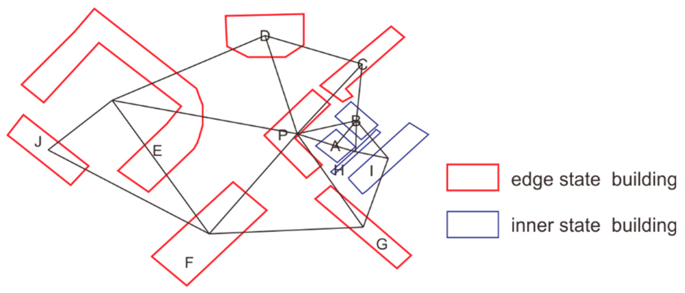
Figure 2.
P building and its K-NN neighborhoods.
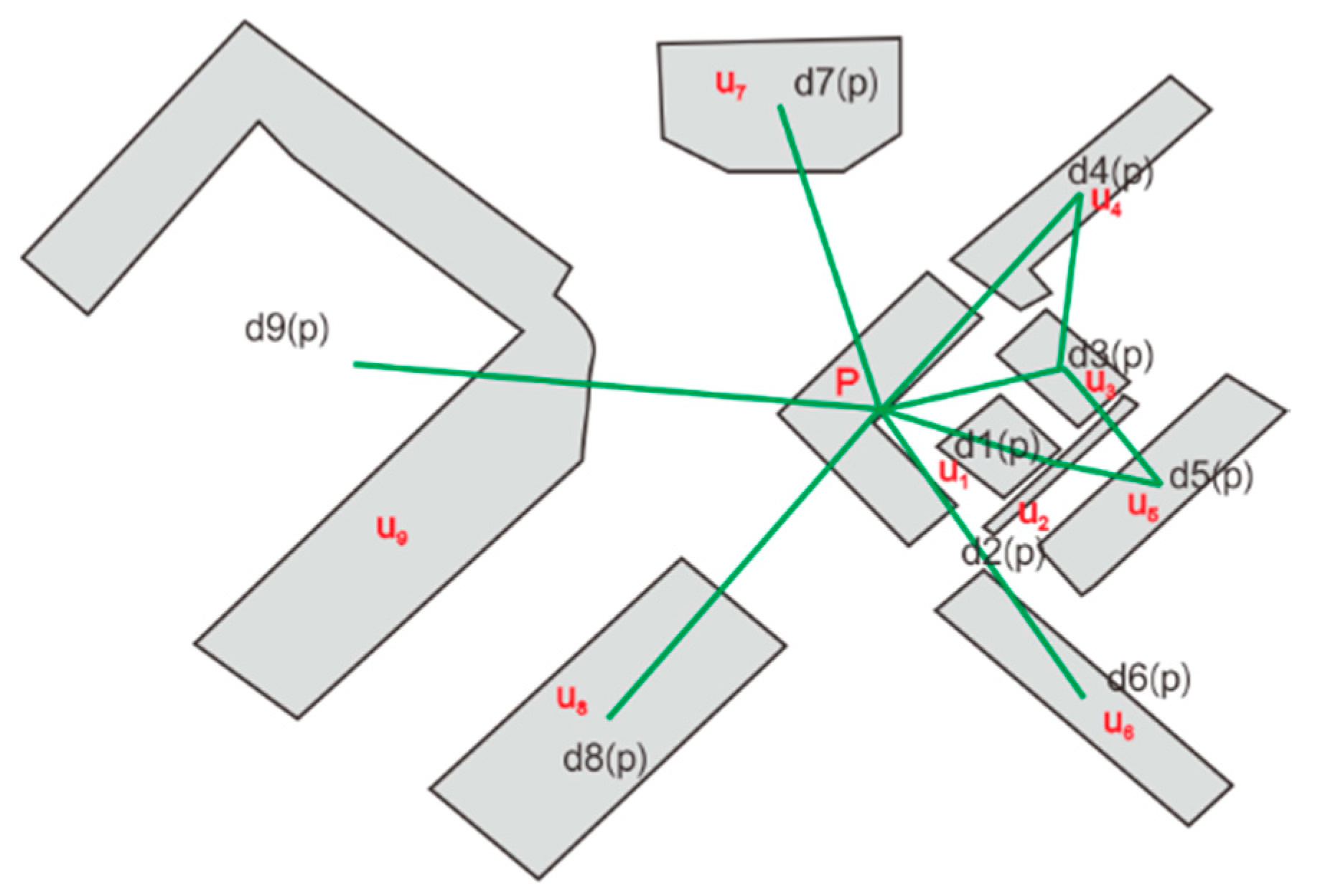
Figure 3.
The center_devia and first_neighbor_avg_r characters of building P.
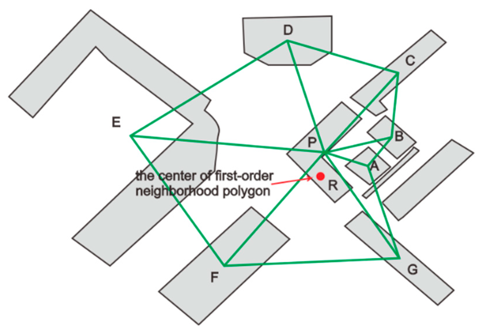
Figure 5.
Building A and its surrounding four buildings.
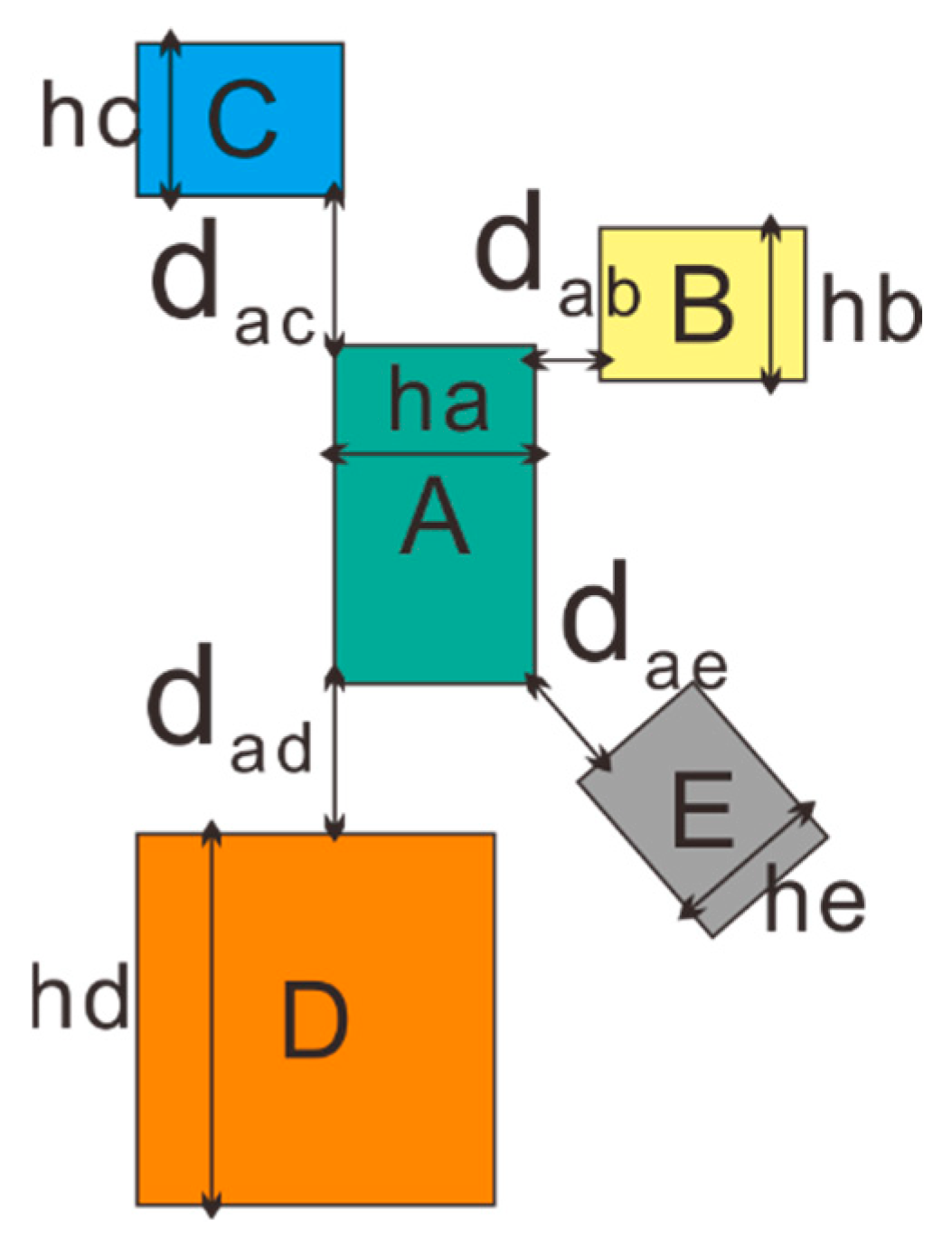
Figure 6.
The DGI model.
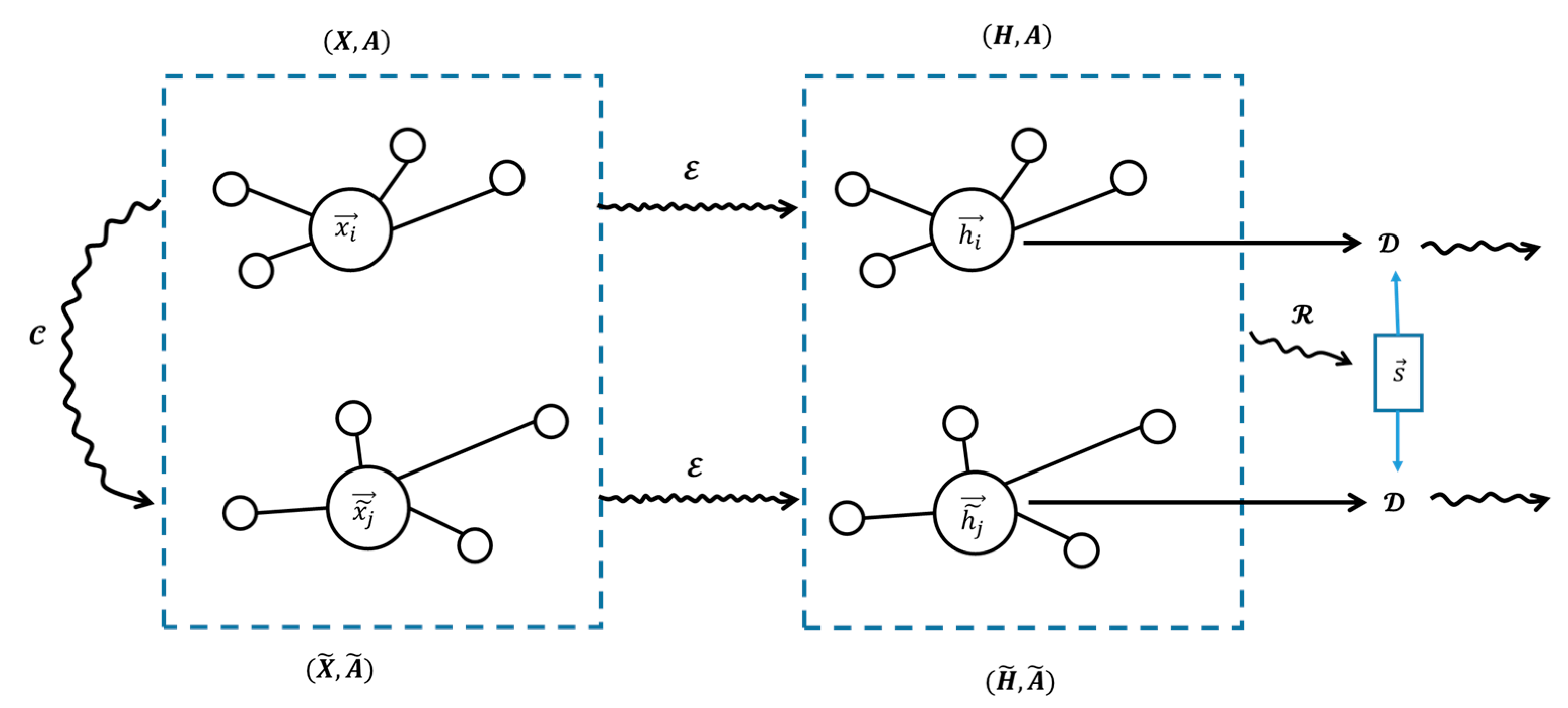
Figure 8.
The experiment data, (a) train dataset from the CD dataset (b) test1 data from the CD dataset, (c) test2 data from the NC dataset.
Figure 8.
The experiment data, (a) train dataset from the CD dataset (b) test1 data from the CD dataset, (c) test2 data from the NC dataset.
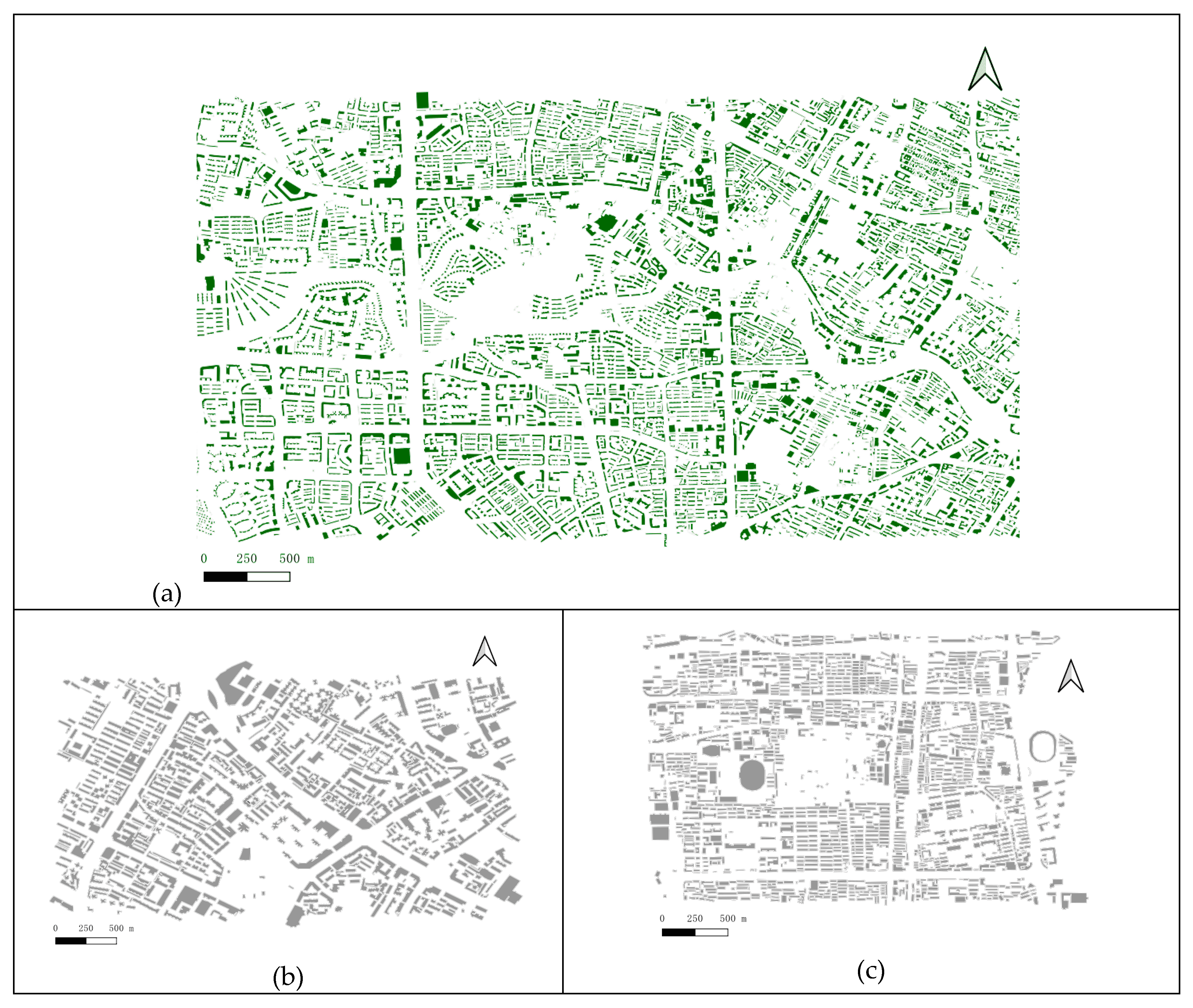
Figure 9.
The training loss diagram for eight feature combinations.
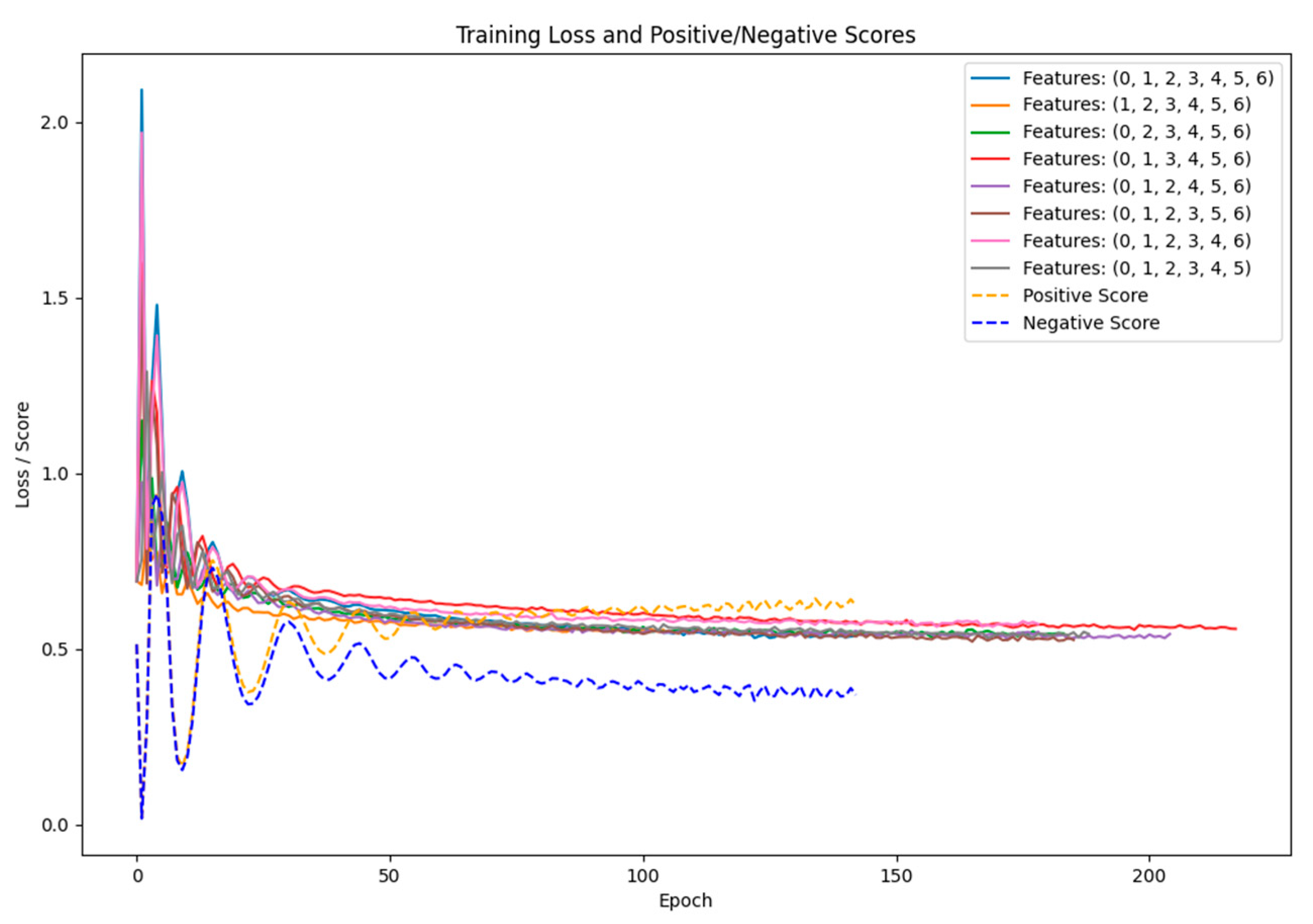
Figure 10.
Evaluation diagram of edge state buildings and inner state buildings (the blue column is pecision, the green column is recall, and the red column is F1-score).
Figure 10.
Evaluation diagram of edge state buildings and inner state buildings (the blue column is pecision, the green column is recall, and the red column is F1-score).
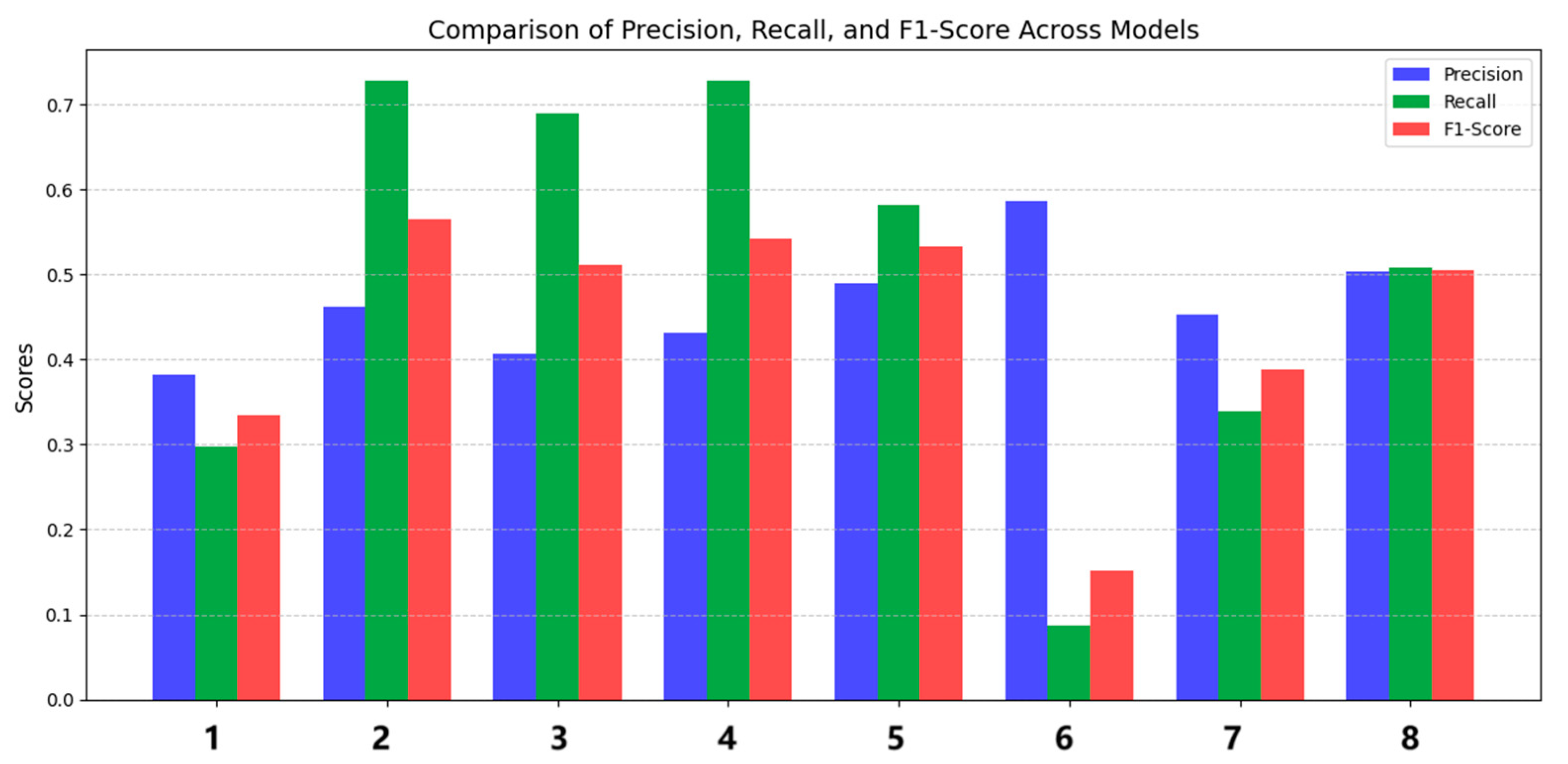
Figure 11.
The binary classification results of edge and inner state buildings: (a) test 1; (b) test 2.
Figure 11.
The binary classification results of edge and inner state buildings: (a) test 1; (b) test 2.
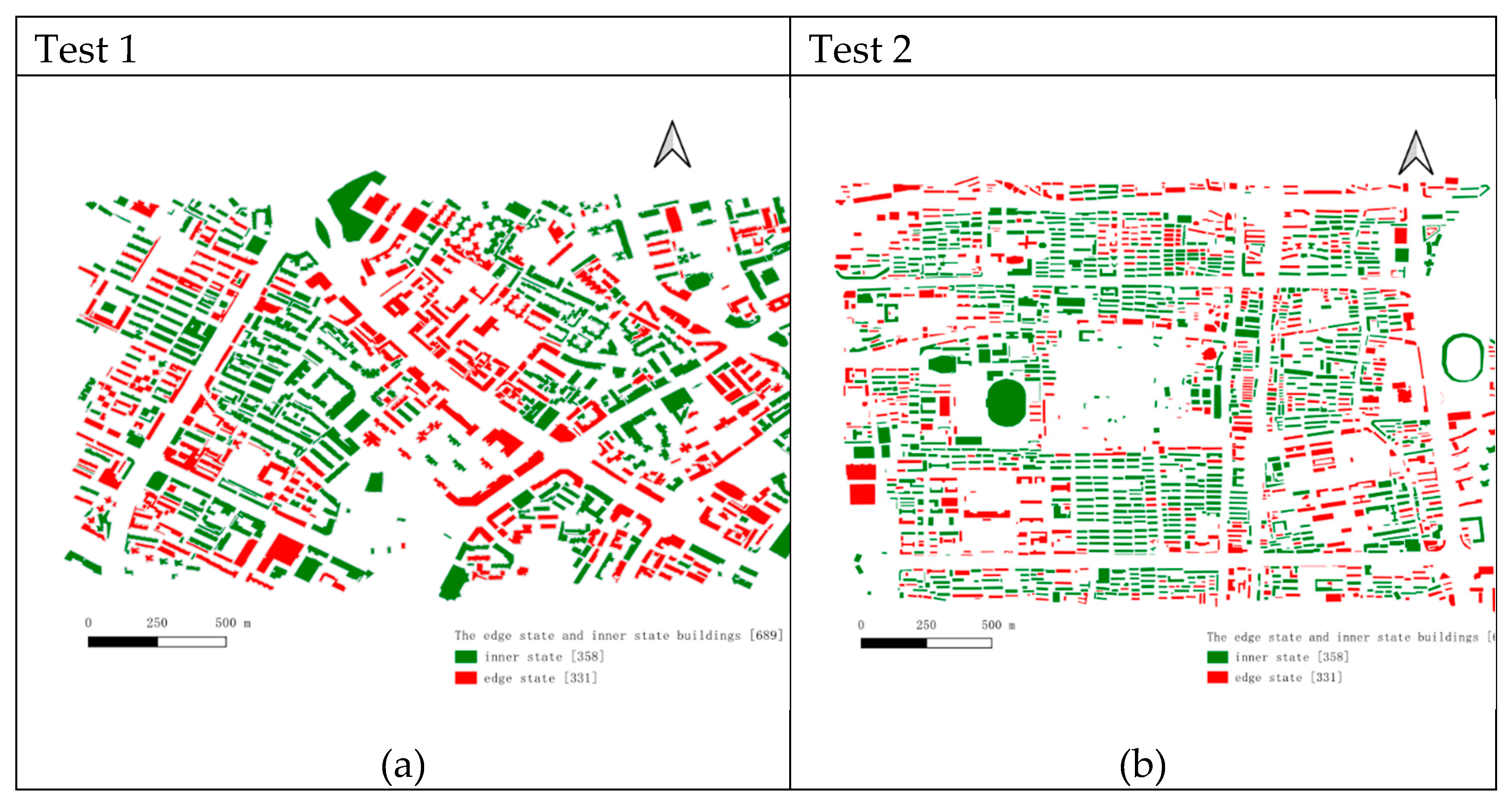
Figure 12.
Clustering results of test data: (a) DGI-EIC on test 1; (b) DGI-EIC on test 2; (c) CDC on test 1; (d) CDC on test 2; (e) MGP on test 1; (f) MGP on test 2.
Figure 12.
Clustering results of test data: (a) DGI-EIC on test 1; (b) DGI-EIC on test 2; (c) CDC on test 1; (d) CDC on test 2; (e) MGP on test 1; (f) MGP on test 2.
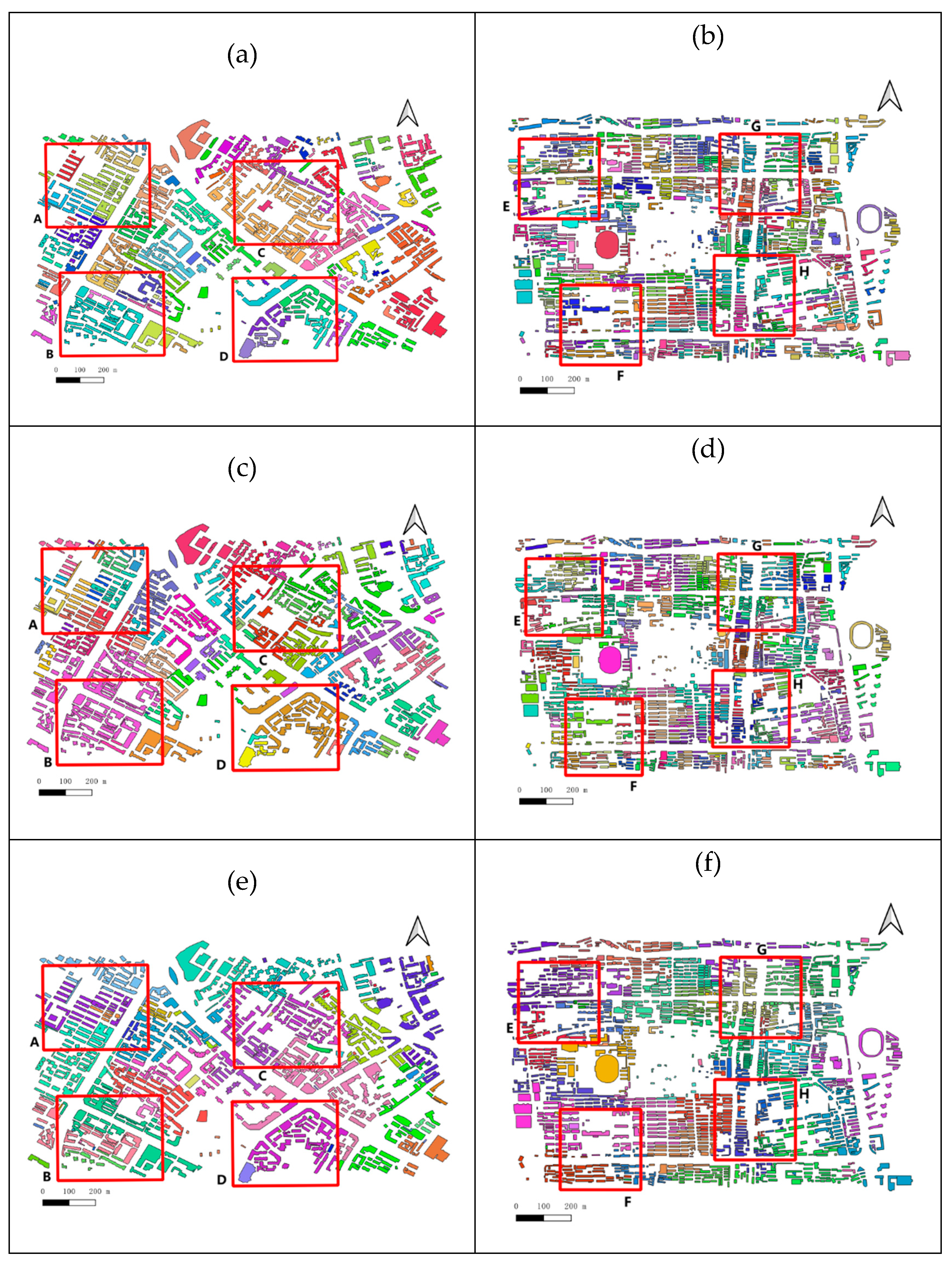
Figure 13.
Clustering details of test 1; (a) DGI-EIC; (b) DGI-EIC; (c) DGI-EIC; (d)DGI-EIC; (e) CDC; (f) CDC; (g) CDC; (h) CDC; (i) MGP; (j) MGP; (k) MGP; (l) MGP.
Figure 13.
Clustering details of test 1; (a) DGI-EIC; (b) DGI-EIC; (c) DGI-EIC; (d)DGI-EIC; (e) CDC; (f) CDC; (g) CDC; (h) CDC; (i) MGP; (j) MGP; (k) MGP; (l) MGP.
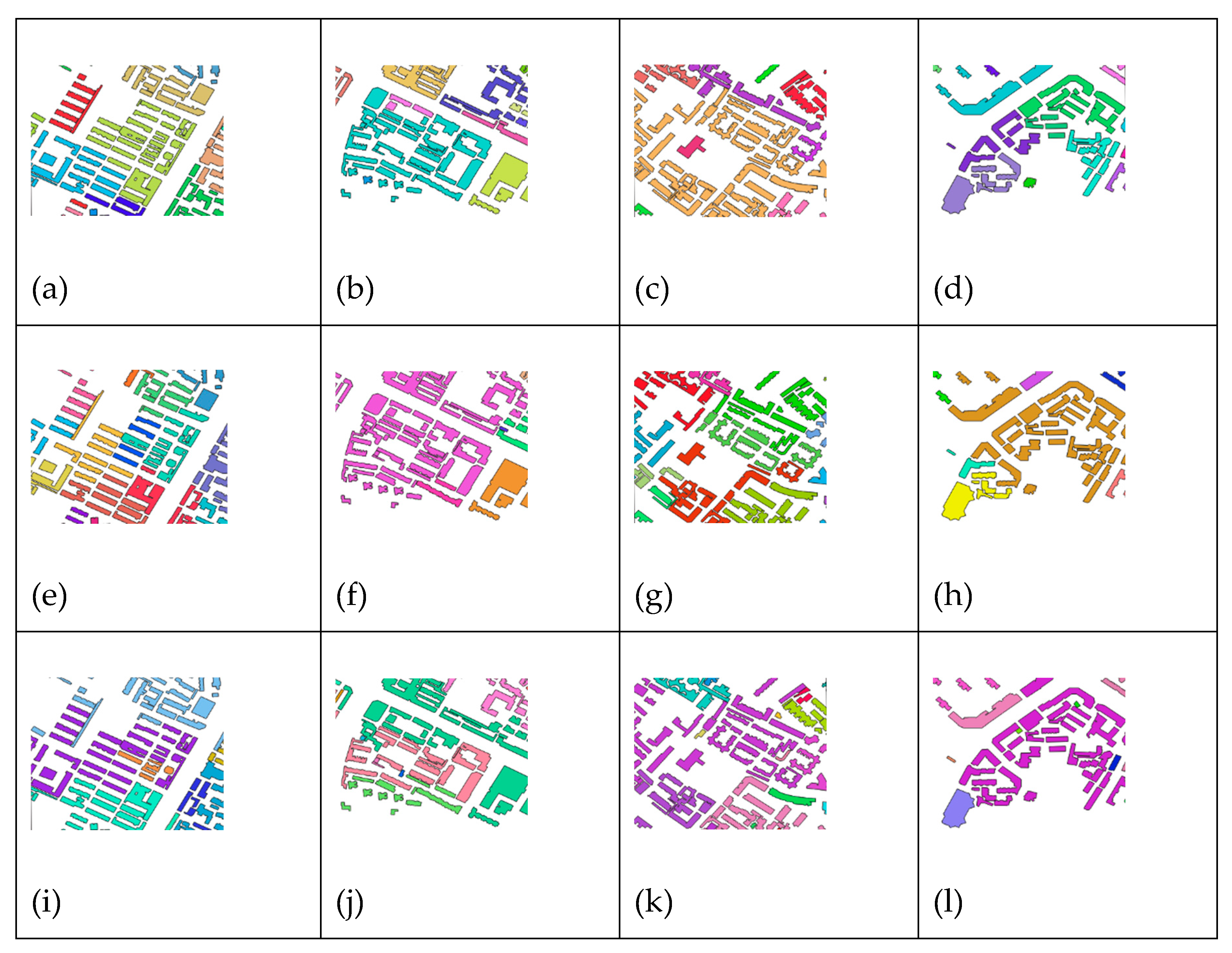
Figure 14.
Clustering details of Test 2: (a) DGI-EIC; (b) DGI-EIC; (c) DGI-EIC; (d)DGI-EIC; (e) CDC; (f) CDC; (g) CDC; (h) CDC; (i) MGP; (j) MGP; (k) MGP; (l) MGP.
Figure 14.
Clustering details of Test 2: (a) DGI-EIC; (b) DGI-EIC; (c) DGI-EIC; (d)DGI-EIC; (e) CDC; (f) CDC; (g) CDC; (h) CDC; (i) MGP; (j) MGP; (k) MGP; (l) MGP.
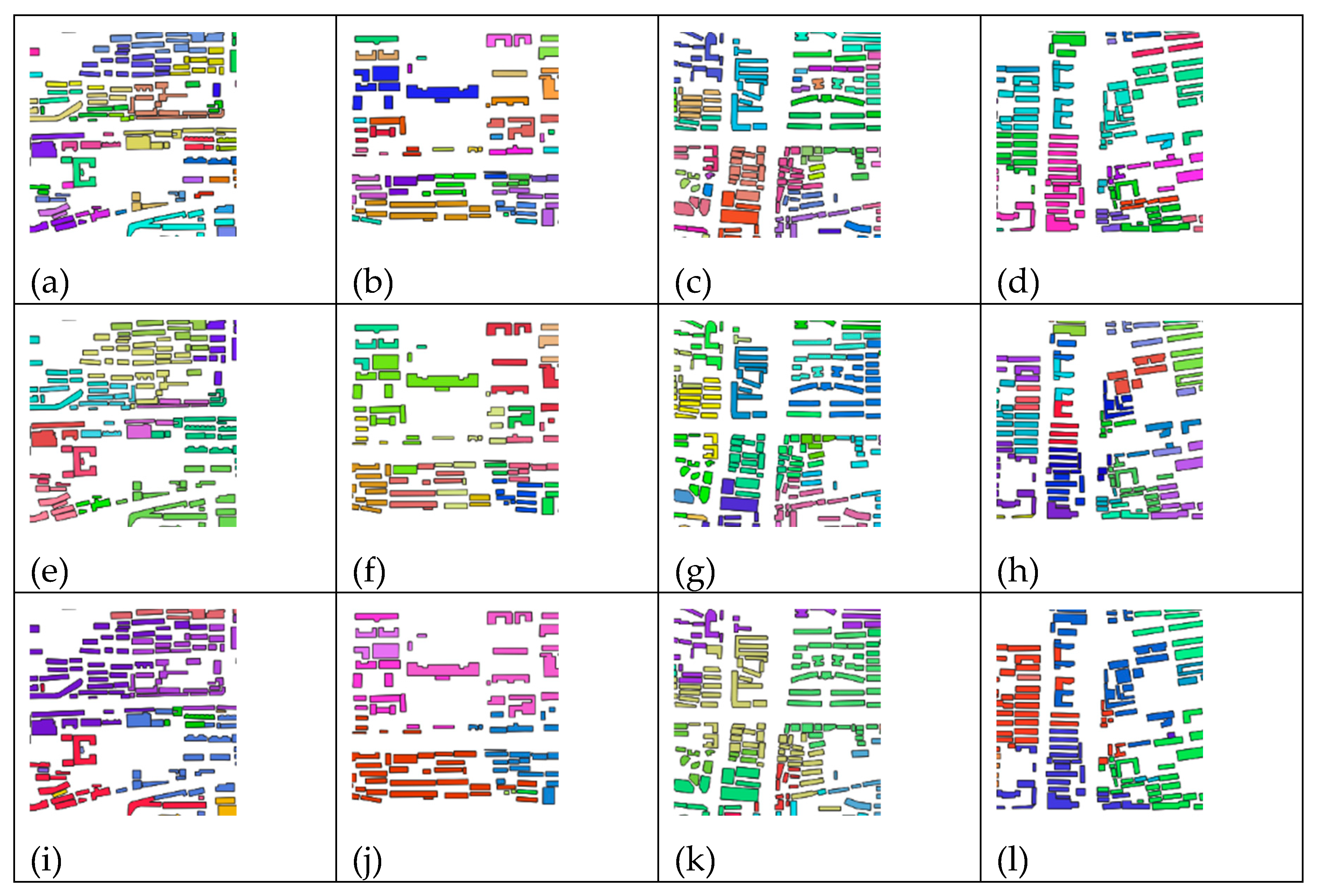

Table 1.
Characteristics to determine edge state building.
| Number | Name | Notation/equation | Description |
| 1 | concavity | The area ratio of the building to its convex hull [36] | |
| 2 | LOF | Section 2.1.2 | |
| 3 | Density | The area of the building is divided by the area of the Voronoi map unit where it is located [37] | |
| 4 | vo_to_b_length | The vector length of the Voronoi graph unit center pointing to the center of the building it contains | |
| 5 | center_devia | Illustrated in Section 2.1.3 | |
| 6 | first_neighbor_avg_r, | - | Average radius of first-order neighborhood polygons of a building |
| 7 | M_dis_cv | Illustrated in Section 2.1.5 |
Table 2.
The percent of concave and rectangular buildings in the experiment data.
| Dataset | Number of Buildings | Percent of Concave Polygon (%) | Percent of Rectangles (ERI index [36]) (%), | Location |
| Training | 4851 | 91.4 | 17.3 | 104.00E,30.66N |
| Test1 | 689 | 94.0 | 16.5 | 104.05E,30.68N |
| Test2 | 1737 | 19.3 | 82.5 | 117.08.E, 28.68。N |
Table 3.
The training of different feature combinations.
| Training number | Feature combination used in training | Feature combination description |
|---|---|---|
| 1 | [concavity,lof,density,vo_to_b_length,center_devia,first_neighbor_avg_r] | Remove m_dis_cv from all seven features |
| 2 | [concavity,lof,density,vo_to_b_length,center_devia , m_dis_cv] | Remove first_neighbor_avg_r from all seven features |
| 3 | [concavity,lof,density,vo_to_b_length ,first_neighbor_avg_r, m_dis_cv] | Remove center_devia from all seven features |
| 4 | [concavity,lof,density ,center_devia,first_neighbor_avg_r, m_dis_cv] | Remove vo_to_b_length from all seven features, |
| 5 | [concavity,lof ,vo_to_b_length,center_devia,first_neighbor_avg_r, m_dis_cv] | Remove density from all seven features, |
| 6 | [concavity ,density,vo_to_b_length,center_devia,first_neighbor_avg_r, m_dis_cv] | Remove lof from all seven features |
| 7 | [lof,density,vo_to_b_length,center_devia,first_neighbor_avg_r, m_dis_cv] | Remove concavity from all seven features |
| 8 | [concavity,lof,density,vo_to_b_length,center_devia,first_neighbor_avg_r, m_dis_cv] | All seven features |
Table 4.
Evaluation of clustering results of test 1 and test 2.
| Experiment data | Method | silhouette coefficient, | davies bouldin index | calinski harabasz index, | ARI |
| Test 1 | DGI-EIC | -0.44 | 4.03 | 5.15 | 0.45 |
| CDC | -0.37 | 4.52 | 5.90 | 0.32 | |
| MGP | -0.46 | 2.26 | 5.70 | 0.37 | |
| Test 2 | DGI-EIC | -0.35 | 3.79 | 5.52 | 0.20 |
| CDC | -0.23 | 3.89 | 10.53 | 0.26 | |
| MGP | -0.35 | 2.12 | 14.93 | 0.37 |
Disclaimer/Publisher’s Note: The statements, opinions and data contained in all publications are solely those of the individual author(s) and contributor(s) and not of MDPI and/or the editor(s). MDPI and/or the editor(s) disclaim responsibility for any injury to people or property resulting from any ideas, methods, instructions or products referred to in the content. |
© 2025 by the authors. Licensee MDPI, Basel, Switzerland. This article is an open access article distributed under the terms and conditions of the Creative Commons Attribution (CC BY) license (http://creativecommons.org/licenses/by/4.0/).
Copyright: This open access article is published under a Creative Commons CC BY 4.0 license, which permit the free download, distribution, and reuse, provided that the author and preprint are cited in any reuse.


