
Submitted:
27 April 2025
Posted:
28 April 2025
You are already at the latest version
Abstract
Batch flotation tests were conducted to recover copper minerals by flotation. Seven flotation intervals (cumulative flotation times) were chosen to characterize flotation kinetics in terms of maximum recoveries, R∞, and flotation rate distributions, f(k). The responses were subsampled, removing one datapoint at a time to obtain seven datasets with six time-recovery data. These datasets were fitted to the Single Flotation Rate, Rectangular and Gamma models. The R∞-f(k) pairs proved to be sensitive to changes in the flotation intervals, particularly under poor model fitting. A simplified scale-up procedure was performed, showing significant uncertainties in the predicted recoveries when the R∞-f(k) pairs were strongly influenced by different flotation intervals.
Keywords:
flotation kinetics
; batch flotation
; kinetic modelling
; flotation rate distribution
; maximum recovery
; scale-up
1. Introduction
Flotation has extensively been used for the separation and concentration of valuable and hydrophobic minerals. The wide range of feed properties and operating conditions, such as mineral liberation, particle size, gas flowrate, froth depth and reagent dosage, as well as the three-phase nature of the process, makes flotation modelling not straightforward [1,2]. This modelling implies the development of mathematical representations that describe the interactions among multiple variables, incorporating implicitly or explicitly critical phenomena that occur in the separation process. These representations are typically based on kinetic, empirical, or first-principle models [3,4,5], from which the former have received special attention due to their applicability for scaling-up purposes.
Kinetic modelling is used to simulate and predict flotation performances under variations in feed properties, changes in reagent schemes and dosages, evaluation of different control strategies, changes in machine geometry and circuits, just to name a few [3]. These models are also used to optimize operating conditions for an adequate trade-off between grade and recovery. Although significant progresses have been made in flotation modelling, difficulties persist in predicting metallurgical results from physical and chemical phenomena related to the collection and separation subprocesses. Thus, kinetic modelling continues to be one of the most used strategies in flotation characterization.
The kinetic model of Equation (1) was originally proposed by Garcia-Zuñiga [6] for batch flotation, establishing a first-order exponential relationship for the cumulative recovery R(t) as a function of the cumulative time, t.
Within Equation (1), R∞ is the maximum recovery and k the flotation rate constant, which was assumed deterministic.
The Single Flotation Rate (SFR) model of Equation (1) has been considered as a suitable representation for modelling flotation kinetics; however, its applicability has proven to be limited mainly due to the distributed nature of the particle properties in flotation feeds [7]. Thus, a flotation rate distribution, f(k), was initially proposed by Imaizumi and Inoue [8] to generalize Equation (1) as a continuous sum of exponential responses, as shown in Equation (2). From this approach, different probability density functions, such as Rectangular [9], Triangular [10], Gamma [8], Exponential [11], Normal [12], among others, have been assumed in literature for f(k).
Particularly, the Rectangular model assumes a uniform f(k) in the range 0 to kmax [9,13], and has commonly led to satisfactory results in the model fitting, keeping only two parameters. From this representation, the resulting R(t) model is given by Equation (3):
The Gamma f(k) proposed by Imaizumi and Inoue [8] has proven to have the required flexibility in describing the heterogeneity of the flotation process [14]. It generalizes Normal and Exponential distributions and can also represent the deterministic case of Equation (1). Equation (4) corresponds to the Gamma f(k), in which aG and kG are shape and scale parameters, respectively, and Γ is the Gamma function. The additional parameter of this f(k), with respect to the Rectangular and SFR models, allows for the simultaneous representation of particles with high and low floatability. The average rate constant kave is obtained from the model parameters, such that kave = kG aG.
From the evaluation of Equation (4) in Equation (2), the R(t) model of Equation (5) is obtained.
The kinetic parameters of Equations (1), (3) and (5) [R∞-f(k) pairs] are obtained from batch flotation tests, and the large-scale results are predicted by applying Equation (6) for continuous systems [15]. Within Equation (6), ξ(t) corresponds to the residence time distribution, which describes the mixing regime of the studied machine or circuit.
In scale-up procedures, the large-scale rate constants are typically corrected based on a scale-up factor, kbatch/kplant, which has been mostly assumed in the range 1.5-3.0 [16]. This factor accounts for all differences between industrial flotation systems and the experimental conditions at laboratory scale [17].
Although kinetic modelling may lead to adequate fitting under specific experimental conditions, some uncertainties persist due to non-standard flotation protocols or poor experimental designs [18,19]. Improvements in kinetic characterizations have been widely reported in literature, with focus on sample representativeness, automation in the concentrate removals, decrease in data variance, among others [19,20,21]. However, the definition of flotation intervals for concentrate removals in batch tests and its effect on the R∞-f(k) estimations have not received special attention, only being assessed under theoretical conditions by Xiao and Vien [22]. Three flotation models were assessed in that study, emulating the application of a D-optimal design in the parameter estimation. Experiments with the same number of datapoints as model parameters were assumed. In addition, independence and homoscedasticity were assumed, conditions that are not satisfied in kinetic responses [19,23]. Although this study presented some limitations, the impact of the definition of flotation times (intervals) on the parameter estimation was for the first time discussed in kinetic characterizations. The methodology reported by Xiao and Vien [22] was subsequently used by Yianatos and Henríquez [24] to define a short-cut approach for the estimation of flotation rates in industrial banks from two mass balances: one mass balance to the overall bank and one mass balance to the first flotation cell. The approach was applied in a rougher flotation circuit, using a Rectangular distribution of rate constants.
This paper evaluates the sensitivity of kinetic characterizations to different selections of flotation intervals in batch tests. From kinetic responses with n time-recovery data, the R∞-f(k) pairs obtained from all possible responses of (n – 1) datasets are evaluated using the R(t) models of Equations (1), (3) and (5). The R∞-f(k) estimates obtained from the sub-sampled kinetic responses are compared to those from the entire dataset (n datapoints). This sensitivity analysis, under moderate changes in the flotation intervals, allows the robustness of an experimental design for the R∞-f(k) estimations to be evaluated. In addition, the variability in the recovery predictions from a scale-up procedure is illustrated under uncertainties in the R∞-f(k) pairs caused by an arbitrary selection of the flotation times in kinetic tests.
2. Materials and Methods
2.1. Sample Preparation and Flotation Tests
Crushed samples of a copper ore were used in the kinetic tests. The 95% confidence interval for the mean of the Cu grade was 0.92 ± 0.08%. The samples were previously crushed, and after quartering, homogenization and splitting procedures, 1-kg sub-samples were prepared for grinding. Dry grinding was performed in a Joy Denver® rod mill (Joy Manufacturing Company, Denver Equipment Division, USA). The grinding times were set at 3.8 min, 5.5 min and 5.8 min to obtain P80s of 300 μm, 212 μm and 150 μm, respectively.
The ground product was poured into a 2.7 L EDEMET flotation cell. Tap water was added to obtain a solid percentage of 33% w/w, and pH was set and kept at 9.5 by adding a lime slurry. Hostaflot 18275 (Clariant Mining Solutions, USA) was used as a collector at 22.5 g/t, with a conditioning time of 5.0 min, whereas Aerofroth 70 (Cytec, USA) was used as a frother at 24 mg/L, and conditioned for 2.5 min. The flotation cell was operated at 700 rpm, with a constant air flowrate of 8 L/min. Seven concentrates were sampled at cumulative times of 0.5, 1.5, 4, 10, 16, 24, and 32 min. Three repetitions were conducted for each experimental condition.
The flotation products were filtered and dried at 90°C. Digested subsamples of each product were filtered, diluted, and analysed by atomic absorption spectrophotometry in a SpectrAA 55 spectrometer (Varian Inc., USA). All feed and product grades were determined for the studied conditions. From the measured Cu grades and the incremental mass recoveries, data reconciliation was performed according to the procedure described by Vinnett, et al. [25]. The average and standard deviation of the time-recovery data are presented in Appendix A.
2.2. Model Fitting and Sensitivity Analysis
Non-linear regression was implemented to obtain all model parameters of Equations (1), (3) and (5). These regressions were performed in Matlab, using the Statistics and Machine Learning Toolbox version 12.3 (The MathWorks, USA). The least-squares estimation problem of Equation (7) was applied, subject to the constraint that R∞ ≤ 100%. Within Equation (7), Rdata is the measured recovery, Rmod is the modelled recovery, ti is the i-th flotation time (cumulative), and n is the number of evaluated datapoints.
The model parameters (R∞, k, kmax, aG, and kG) were first estimated for the entire time-recovery dataset (baseline, with 7 datapoints). Secondly, new regressions were carried out, omitting one data point at a time to perform a sensitivity analysis under sub-sampled kinetic responses. In this analysis, all model parameters were re-estimated as depicted in Figure 1. In this schematic, a cross indicates that that specific datapoint was skipped from the time-recovery dataset for the new R∞-f(k) estimations. Although the approach of removing one data point at a time has previously been employed in assessing flotation kinetics, its use has only been focused on model cross-validation [26,27,28], not evaluating the sensitivity or uncertainties in the R∞-f(k) estimations.
3. Results
The R(t) models of Equations (1), (3) and (5) were fitted to the entire time-recovery datasets, from which reference R∞-f(k) pairs were obtained (baseline kinetic parameters). Figure 2 shows the R(t) model fitting for the three evaluated experimental conditions [Figure 2(a) for P80 = 150 μm, Figure 2(b) for P80 = 212 μm, and Figure 2(c) for P80 = 300 μm], assuming the Single Flotation Rate, Rectangular and Gamma models. The root mean squared errors (RMSEs) are presented as indicators of the magnitude of the modelling errors. The deterministic flotation rate of Equation (1) consistently led to the poorest kinetic representation for the experimental data.
A sensitivity analysis was conducted using the procedure schematized in Figure 1. Figures 3 shows the model fitting, using the SFR model of Equation (1). Figure 3(a) presents the baseline condition, with no data removal. Figures 3(b) to 3(h) show the model fitting after removing one datapoint at a time. From these results, the sensitivity of the R∞-f(k) estimates under moderate changes in the flotation intervals was studied.
Figure 4 presents all the estimated f(k)s for the three evaluated experimental conditions. Figures 4(a), 4(d) and 4(g) present the estimated rate constants of the SFR model, Figures 4(b), 4(e) and 4(h) the Rectangular f(k)s, and Figures 4(c), 4(f) and 4(i) the Gamma f(k)s. The baseline f(k)s are shown as solid black lines, whereas the f(k)s from the sensitivity analysis are presented as coloured dotted lines. In the plot legends, Sens. n indicates that the n-th datapoint was omitted in the parameter estimation.
The SFR and Rectangular models, in most cases, presented a high parameter sensitivity to the experimental design, specifically to the first two flotation intervals in the batch tests (Sens. 1 and Sens. 2). When individually omitting these datapoints, the k and kmax values [Equations (1) and (3), respectively] presented significant deviations regarding the baseline; however, Test 3 led to more robust estimates from the deterministic rate constant [Figure 4(g)]. Removing time-recovery data from the third flotation interval did not lead to significant changes in the SFR and Rectangular f(k)s with respect to the baseline. Results for the SFR and Rectangular models indicate that using 6 datapoints in the kinetic tests will lead to uncertainties in the flotation rate parameters, particularly due to a poor characterization of the recovery rates at the beginning of the process. Thus, the results from Figure 4 suggest that additional flotation intervals must be included at short flotation times to guarantee more accurate k and kmax estimations. For Tests 1 and 2, the Gamma model of Equation (5) presented remarkably higher robustness compared to the SFR and Rectangular models. The location, dispersion, and shapes of these estimated f(k)s were not critically modified regarding the baseline. However, Test 3 led to unstable f(k) estimates from the Gamma model. This model has an additional parameter, which makes it more prone to overfitting, especially for noisy kinetic responses. Indeed, Figure 2(c) shows that the Gamma model presented poorer model fitting in Test 3, with respect to the first two experimental conditions. This result is mainly attributable to the more irregular time-recovery trends between the second and fourth datapoints in Figure 2(c), and the higher flexibility of the Gamma model. As a result, removing the first datapoint significantly impacted the f(k) shape, and thus, the flotation rate characterization.
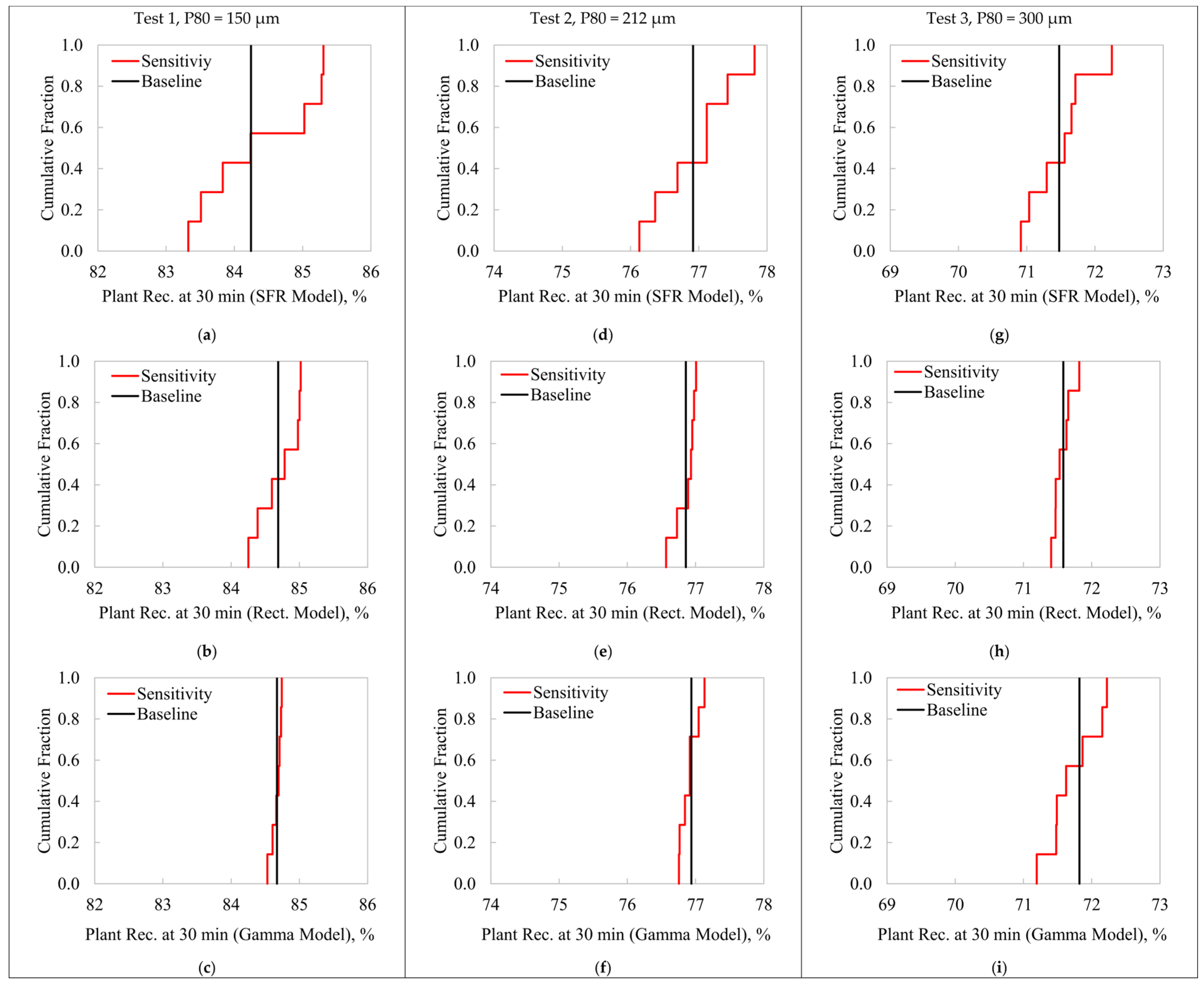
Figure 5 presents the variability in the R∞ estimations when applying the sensitivity analysis, using the SFR [Figures 5(a), 5(d) and 5(g)], Rectangular [Figures 5(b), 5(e) and 5(h)] and Gamma [Figures 5(c), 5(f) and 5(i)] models for the studied experimental conditions. The R∞ estimates when removing one data point at a time are presented as cumulative distribution functions. The vertical continuous black lines represent the R∞ values obtained in the baseline, with the entire dataset. As a reference, the measured cumulative recovery at t = 32 min [R(32)] are also deployed as a vertical blue line (dashed). In all cases, the SFR model led to R∞ estimations significantly lower than the measured recovery at the end of the process, R(32). This inconsistency indicates the limitation of Equation (1) to characterize this flotation process. For Tests 1 and 2, the Rectangular model also led to R∞ values lower than R(32); however, the differences are significantly lower than those observed with the SFR model. Similarly, the Gamma model presented inconsistencies in the R∞ estimates with respect to the experimental data in Test 3, in agreement with the unstable f(k)s shown in Figure 4(i).
The SFR model consistently led to high variability in the R∞ estimation. The comparative results between the Rectangular and Gamma models in terms of the R∞ precision depended on the experimental conditions. In Test 1, the Gamma R∞ estimations were more stable than those obtained from the Rectangular model. However, poor R∞ estimations were obtained in Test 3 with the Gamma approach due to the noisier kinetic response and the higher flexibility of this model structure. In Test 2, the Rectangular model led to slightly lower R∞ variability with respect to the Gamma model, though the maximum recovery values tended to be lower than the experimental recoveries at the end of the process.
An overall comparison of the kinetic representations states that the most robust approach in terms of the R∞-f(k) stability depends on the experimental conditions. Test 1 was adequately described by the Gamma model, with negligible changes in the parameter estimation under moderate changes in the selection of flotation times. Test 3, on the other hand, had a more stable and consistent R∞-f(k) estimations using the Rectangular model. Although both the Rectangular and Gamma models presented comparable results for Test 2, the more consistent R∞ estimations with the experimental recoveries R(32) gave a slight advantage to the latter.
The R∞-f(k) estimations of Figure 4 and Figure 5 were used to analyze the impact of the parameter uncertainties on the scale-up results, under moderate changes in the flotation intervals in the laboratory tests. For illustration purposes, 6 flotation cells in series were considered at large scale, in which each machine was assumed as a perfect mixer for the residence time distribution ξ(t) in Eq. (6). A rougher circuit with a total flotation time of 20 min was evaluated, implying a mean residence time of 3.33 min per cell. A scale-up factor of 2.5 was used as typically reported in literature [16]. Thus, for the SFR and Rectangular models, the rate parameters k/2.5 and kmax/2.5 were used when evaluating Eq. (6). For the Gamma model, the average rate constant was set to kave/2.5 at large scale, keeping the same f(k) shapes as in Figures 4(c), 4(f) and 4(i). This assumption considers that aG in Equation (4) did not change between the evaluated scales. It should be mentioned that the scale-up procedures assuming the SFR and Rectangular models are straightforward as closed expressions for the large-scale recoveries can be obtained [17,29]. For the Gamma model, numerical integration is required.
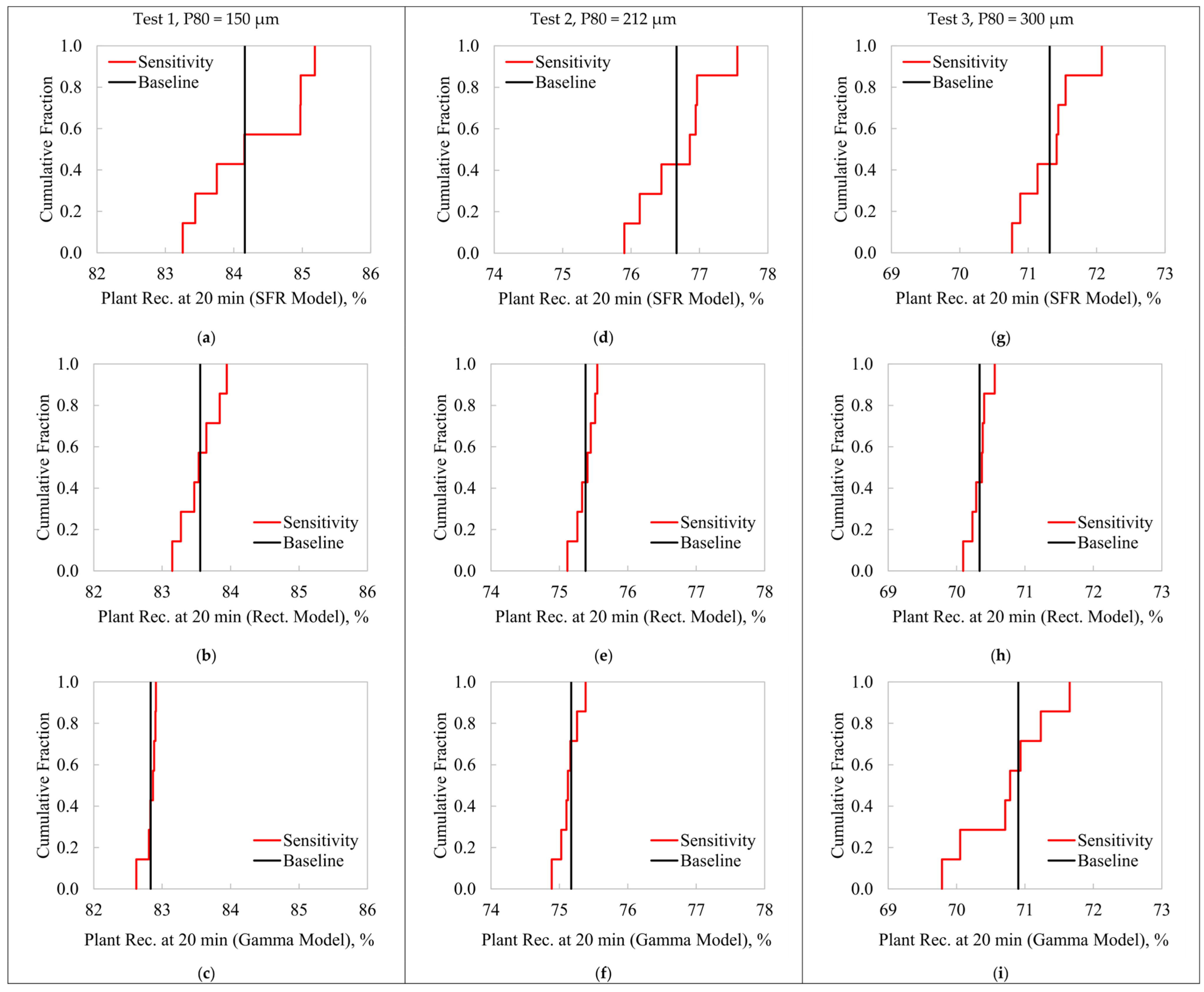
Figure 6 presents the scale-up results at 20 min using the lab-scale kinetic characterizations in the baseline and from the sensitivity analysis, assuming the SFR [Figures 6(a), 6(d) and 6(g)], Rectangular [Figures 6(b), 6(e) and 6(h)] and Gamma [Figures 6(c), 6(f) and 6(i)] models for the three feed P80s. All recoveries are presented as cumulative distribution functions. Figure B1 of Appendix B shows the same results for a large-scale residence time of 30 min, again considering 6 perfect mixers in series (mean residence time of 5.0 min per cell). The SFR model led to a high variability and high correlation with the maximum recoveries depicted in Figures 5(a), 5(d) and 5(g). As pure exponential trends rapidly converge to steady values, it is expected that scaling-up procedures with relatively long flotation times tend to R∞. As these maximum recoveries were highly sensitive to the chosen flotation intervals in the laboratory tests, and their values were inconsistent with the experimental data, the SFR model structure is not recommended for scaling-up this flotation process. Indeed, any flotation system presenting sustained increasing trends at long flotation times will not be well represented by Equation (1), discarding this model for scale-up purposes. It should be noted that the scaled-up SFR recoveries were significantly higher than those obtained from the Rectangular and Gamma models, again justified by the SFR convergence to the maximum recoveries. The uncertainties of the scaled-up recoveries when assuming the Rectangular and Gamma models agreed with the stabilities of the R∞-f(k) estimates shown in Figure 4 and Figure 5. Thus, higher precision was obtained with the Gamma model in Test 1, and this trend was reversed in Test 3. In Test 2, comparable variability was obtained with both models, in agreement with the R∞-f(k) variabilities observed in Figures 4(e), 4(f), 5(e) and 5(f).
An alternative and simplified procedure considers the prediction of large-scale recoveries, scaling-up the lab results based on the flotation times instead of the flotation rates. In this case, given a large-scale residence time τ, the predicted recovery is directly obtained from batch tests at t = τ/f, where f is a scale-up factor [16]. This scale-up factor has proved to be comparable to that from the ratio of batch/plant rate constants [30]. Thus, assuming an f value of 2.5, the large-scale recovery at 20 min can be estimated from the lab-scale recovery at 8 min. Using various interpolation techniques for the experimental data presented in Appendix A, the estimated recoveries of Tests 1, 2 and 3 at t = 8 min (τ = 20 min) were 83%, 75% and 70%, respectively. These values are consistent with the estimated recoveries of Figure 6 for Tests 1 and 2 using the Rectangular and Gamma models, under moderate changes in the flotation intervals. For Test 3, only the Rectangular model led to a consistent estimation with respect to the interpolated recoveries. Again, the SFR model did not lead to recovery estimations that agree with the experimental data, showing the limited kinetic representation obtained from Equation (1).
The results presented here proved the sensitivity of kinetic characterizations to the selection of flotation intervals in laboratory tests. This sensitivity may critically affect the scale-up results for circuit sizing. Particularly, the SFR model not only presented poor model fitting, but also high R∞-k variability and inconsistent scale-up results. Therefore, this model structure is not recommended for flotation systems presenting slight increasing trends at long flotation times. The proposed methodology allows for the detection of opportunities for improvement in experimental designing, detecting the sensitivity of the ∞-f(k) pairs estimated from batch tests. Further developments are being made to establish a systematic procedure for a robust definition of flotation intervals in kinetic characterizations.
4. Conclusions
A sensitivity analysis was conducted for the characterization of flotation kinetics at laboratory scale. The time-recovery data was slightly modified, removing one data point at a time to assess the variability in the parameter estimation, assuming the Single Flotation Rate, Rectangular and Gamma models. The stability of these estimates was used as an indicator of the robustness of the experimental design. The main findings are summarized as follows:
- The classical SFR model not only had poor model fitting but also presented high R∞-k variability under moderate changes in the selection of flotation intervals in the laboratory tests. In addition, the R∞ were consistently lower than the recoveries at the end of the process, given the abrupt decrease of pure exponential decays at long flotation times. As a result, this model structure was inadequate to scale-up metallurgical results, as they converged to R∞, with high variability.
- The Rectangular and Gamma models led to more stable kinetic characterizations. However, the latter also presented high R∞-f(k) uncertainties at a feed P80 = 300 µm, which was attributed to the potential overfitting under noisy kinetic responses when assuming a Gamma model. The parameter stability depended on the experimental conditions. At P80 = 150 µm, the Gamma model led to the highest stability for the R∞-f(k) estimates, whereas at P80 = 300 µm the best results were obtained with the Rectangular approach. At P80 = 212 µm, non-significant differences were obtained with both models, with a slight advantage from the Gamma model due to the consistency between the estimated R∞ and the recovery at the end of the process.
- For scaling-up metallurgical results, the Rectangular and Gamma models kept the same patterns in terms of stability as those of the kinetic parameters. An important feature of both kinetic representations was its consistency with the simplified scale-up approach by flotation/residence time. This consistency was not observed with the classical SFR model, indicating again the poor results typically obtained when assuming pure exponential decays.
The sensitivity analysis presented here proved the significant impact of the selected flotation intervals on kinetic characterizations. As these intervals are, in most cases, arbitrarily chosen in laboratory tests, these findings illustrate the relevance of running optimal experimental designs to minimize R∞-f(k) uncertainties. Further developments are being made to systematically improve kinetic modelling in flotation.
Author Contributions
Conceptualization, L.V.; methodology, L.V. and M.R.; software, L.V., A.E., F.O and M.R.; validation, L.V., A.E., F.O and M.R.; formal analysis, L.V., A.E., F.O and M.R.; investigation, L.V., A.E., F.O and M.R.; resources, L.V.; data curation, L.V. and A.E.; writing—original draft preparation, L.V. and M.B.; writing—review and editing, L.V. and M.B.; visualization, L.V. and M.B.; supervision, L.V.; project administration, L.V.; funding acquisition, L.V. All authors have read and agreed to the published version of the manuscript.
Funding
This research was funded by Agencia Nacional de Investigación y Desarrollo (ANID), Fondecyt de Iniciación 11240125, Chile.
Data Availability Statement
The data presented in this study are available on request from the corresponding author.
Acknowledgments
The authors are grateful to Agencia Nacional de Investigación y Desarrollo. (ANID), Fondecyt de Iniciación 11240125, and Universidad Técnica Federico Santa María, Chile.
Conflicts of Interest
The authors declare no conflicts of interest. The funders had no role in the design of the study; in the collection, analyses, or interpretation of data; in the writing of the manuscript; or in the decision to publish the results.
Appendix A
Table A1 presents the average Cu recoveries and sample standard deviations for the three evaluated tests. Adequate repeatability was obtained. However, a noisier response was obtained in Test 3, which mainly affected the kinetic characterization from the Gamma model, given its higher flexibility and sensitivity to overfitting.

Table A1.
Average copper recoveries and sample standard deviations in the evaluated experimental conditions.
Table A1.
Average copper recoveries and sample standard deviations in the evaluated experimental conditions.
| Test 1, P80 = 150 µm | Test 2, P80 = 212 µm | Test 3, P80 = 300 µm | ||||
|---|---|---|---|---|---|---|
| Flotation Time, min | Average ΦRecovery, % | Standard ΦDeviation, % | Average ΦRecovery, % | Standard ΦDeviation, % | Average ΦRecovery, % | Standard ΦDeviation, % |
| 0.5 | 50.2 | 1.01 | 37.1 | 0.25 | 34.4 | 4.89 |
| 1.5 | 68.9 | 2.25 | 59.2 | 3.20 | 59.4 | 3.43 |
| 4 | 79.8 | 0.69 | 72.0 | 1.25 | 67.6 | 1.64 |
| 10 | 84.3 | 1.31 | 76.2 | 1.40 | 70.6 | 1.56 |
| 16 | 85.9 | 1.44 | 77.8 | 1.38 | 72.2 | 1.73 |
| 24 | 87.2 | 1.52 | 79.1 | 1.41 | 73.2 | 1.78 |
| 32 | 87.9 | 1.59 | 80.0 | 1.42 | 73.7 | 1.85 |
Appendix B
Figure A1 shows the cumulative distribution functions for the scale-up results at 30 min, similarly to Figure 6, assuming the SFR [Figures A1(a), A1(d) andA1(g)], Rectangular [Figures A1(b), A1(e) and A1(h)] and Gamma [Figures A1(c), A1(f) and A1(i)] models. The same patterns as those shown at 20 min are observed in terms of the relative variability. In this case, the scaled-up SFR recoveries converged to the estimated SFR maximum recoveries [R∞ < R(32)] due to the long residence time assumed in the procedure.
Figure A1.
Cumulative distribution functions of the scale-up recoveries at 30 min of continuous flotation, 6 perfect mixers in series: (a) Test 1, P80 = 150 µm, SFR model; (b) Test 1, P80 = 150 µm, Rectangular model; (c) Test 1, P80 = 150 µm, Gamma model; (d) Test 2, P80 = 212 µm, SFR model; (e) Test 2, P80 = 212 µm, Rectangular model; (f) Test 2, P80 = 212 µm, Gamma model; (g) Test 3, P80 = 300 µm, SFR model; (h) Test 3, P80 = 300 µm, Rectangular model; (i) Test 3, P80 = 300 µm, Gamma model.
References
- Bu, X.; Xie, G.; Peng, Y.; Ge, L.; Ni, C. Kinetics of flotation. order of process, rate constant distribution and ultimate recovery. Physicochemical Problems of Mineral Processing 2017, 53, 342–365. [Google Scholar] [CrossRef]
- Bergh, L.; Yianatos, J.; Bravo, G. On-line monitoring of a pilot flotation rougher circuit by using PCA models. IFAC-PapersOnLine 2018, 51, 335–340. [Google Scholar] [CrossRef]
- Gharai, M.; Venugopal, R. Modeling of flotation process—an overview of different approaches. Mineral Processing and Extractive Metallurgy Review 2016, 37, 120–133. [Google Scholar] [CrossRef]
- Villeneuve, J.; Guillaneau, J.C.; Durance, M.V. Flotation modelling: A wide range of solutions for solving industrial problems. Minerals Engineering 1995, 8, 409–420. [Google Scholar] [CrossRef]
- Finch, J.A.; Dobby, G.S. Column flotation: A selected review. Part I. International Journal of Mineral Processing 1991, 33, 343–354. [Google Scholar] [CrossRef]
- Garcia-Zuñiga, H. La recuperación por flotación es una función exponencial del tiempo. Boletín Minero, Sociedad Nacional de Minería 1935, 47, 83–86. [Google Scholar]
- Ofori, P.; O’Brien, G.; Hapugoda, P.; Firth, B. Distributed flotation kinetics models – a new implementation approach for coal flotation. Minerals Engineering 2014, 66–68, 77–83. [Google Scholar] [CrossRef]
- Imaizumi, T.; Inoue, T. Kinetic consideration of froth flotation. In Proceedings of the 6th International Mineral Processing Congress, Cannes, France; 1963; pp. 581–593. [Google Scholar]
- Huber-Panu, I.; Ene-Danalache, E.; Cojocariu, D.G. Mathematical models of batch and continuous flotation. In Flotation--A. M. Gaudin Memorial; American Institute of Mining, Metallurgical, and Petroleum Engineers, Inc.: New York, USA, 1976; Volume 2, pp. 675–724. [Google Scholar]
- Harris, C.; Chakravarti, A. Semi-batch froth flotation kinetics: species distribution analysis. Transactions of the American Institute of Mining, Metallurgical, and Petroleum Engineers 1970, 247, 162–172. [Google Scholar]
- Dowling, E.C.; Klimpel, R.R.; Aplan, F.F. Model discrimination in the flotation of a porphyry copper ore. Minerals and Metallurgical Processing 1985, 2, 87–101. [Google Scholar] [CrossRef]
- Chander, S.; Polat, M. Flotation Kinetics: Methods For Estimating Distribution Of Rate Constants. In Proceedings of the International Mineral Processing Congress (XIX IMPC), San Francisco, USA, 22-27 October, 1995; pp. 105–111. [Google Scholar]
- Klimpel, R.R. Selection of chemical reagents for flotation. In Mineral processing plant design, Mular; A.L., Bhappu, R.B., Eds.; SME-AIME; New York, 1980; Volume 2, pp. 907–934. [Google Scholar]
- Murhula, E.; Hashan, M.; Otsuki, A. Effect of Solid Concentration and Particle Size on the Flotation Kinetics and Entrainment of Quartz and Hematite. Metals 2023, 13. [Google Scholar] [CrossRef]
- Woodburn, E.T.; Loveday, B.K. The effect of variable residence time on the performance of a flotation system. Journal of the Southern African Institute of Mining and Metallurgy 1965, 65, 612–628. [Google Scholar]
- Mesa, D.; Brito-Parada, P.R. Scale-up in froth flotation: A state-of-the-art review. Separation and Purification Technology 2019, 210, 950–962. [Google Scholar] [CrossRef]
- Yianatos, J.; Contreras, F.; Morales, P.; Coddou, F.; Elgueta, H.; Ortíz, J. A novel scale-up approach for mechanical flotation cells. Minerals Engineering 2010, 23, 877–884. [Google Scholar] [CrossRef]
- Sandoval-Zambrano, G.; Montes-Atenas, G. Errors in the estimation of size-by-liberation flotation rate constants. Minerals Engineering 2012, 27, 1–10. [Google Scholar] [CrossRef]
- Napier-Munn, T.J. Statistical methods to compare batch flotation grade-recovery curves and rate constants. Minerals Engineering 2012, 34, 70–77. [Google Scholar] [CrossRef]
- Amelunxen, P.; LaDouceur, R.; Amelunxen, R.; Young, C. A phenomenological model of entrainment and froth recovery for interpreting laboratory flotation kinetics tests. Minerals Engineering 2018, 125, 60–65. [Google Scholar] [CrossRef]
- Ross, V. Key aspects of bench flotation as a geometallurgical characterization tool. Journal of the Southern African Institute of Mining and Metallurgy 2019, 119, 361–367. [Google Scholar] [CrossRef]
- Xiao, Z.; Vien, A. Experimental designs for precise parameter estimation for non-linear models. Minerals Engineering 2004, 17, 431–436. [Google Scholar] [CrossRef]
- Vinnett, L.; Jaques, A.; Alvarez-Silva, M.; Waters, K.E. Incorporating the covariance effect in modelling batch flotation kinetics. Minerals Engineering 2018, 122, 26–37. [Google Scholar] [CrossRef]
- Yianatos, J.B.; Henríquez, F.D. Short-cut method for flotation rates modelling of industrial flotation banks. Minerals Engineering 2006, 19, 1336–1340. [Google Scholar] [CrossRef]
- Vinnett, L.; Yianatos, J.; Flores, S. On the mineral recovery estimation in Cu/Mo flotation plants. Minerals & Metallurgical Processing 2016, 33, 97–106. [Google Scholar] [CrossRef]
- Vinnett, L.; Navarra, A.; Waters, K.E. An inversion approach to characterize batch flotation kinetics. Minerals Engineering 2019, 143, 105944. [Google Scholar] [CrossRef]
- Ni, C.; Bu, X.; Xia, W.; Peng, Y.; Xie, G. Effect of slimes on the flotation recovery and kinetics of coal particles. Fuel 2018, 220, 159–166. [Google Scholar] [CrossRef]
- Polat, M.; Chander, S. First-order flotation kinetics models and methods for estimation of the true distribution of flotation rate constants. International Journal of Mineral Processing 2000, 58, 145–166. [Google Scholar] [CrossRef]
- Yianatos, J.; Vallejos, P. Challenges in flotation scale-up: The impact of flotation kinetics and froth transport. Minerals Engineering 2024, 207, 108541. [Google Scholar] [CrossRef]
- Yianatos, J.B.; Bergh, L.G.; Aguilera, J. Flotation scale up: use of separability curves. Minerals Engineering 2003, 16, 347–352. [Google Scholar] [CrossRef]
Figure 1.
Schematic of removing one data point at a time in the sensitivity analysis for the R∞ and f(k) estimations.
Figure 1.
Schematic of removing one data point at a time in the sensitivity analysis for the R∞ and f(k) estimations.
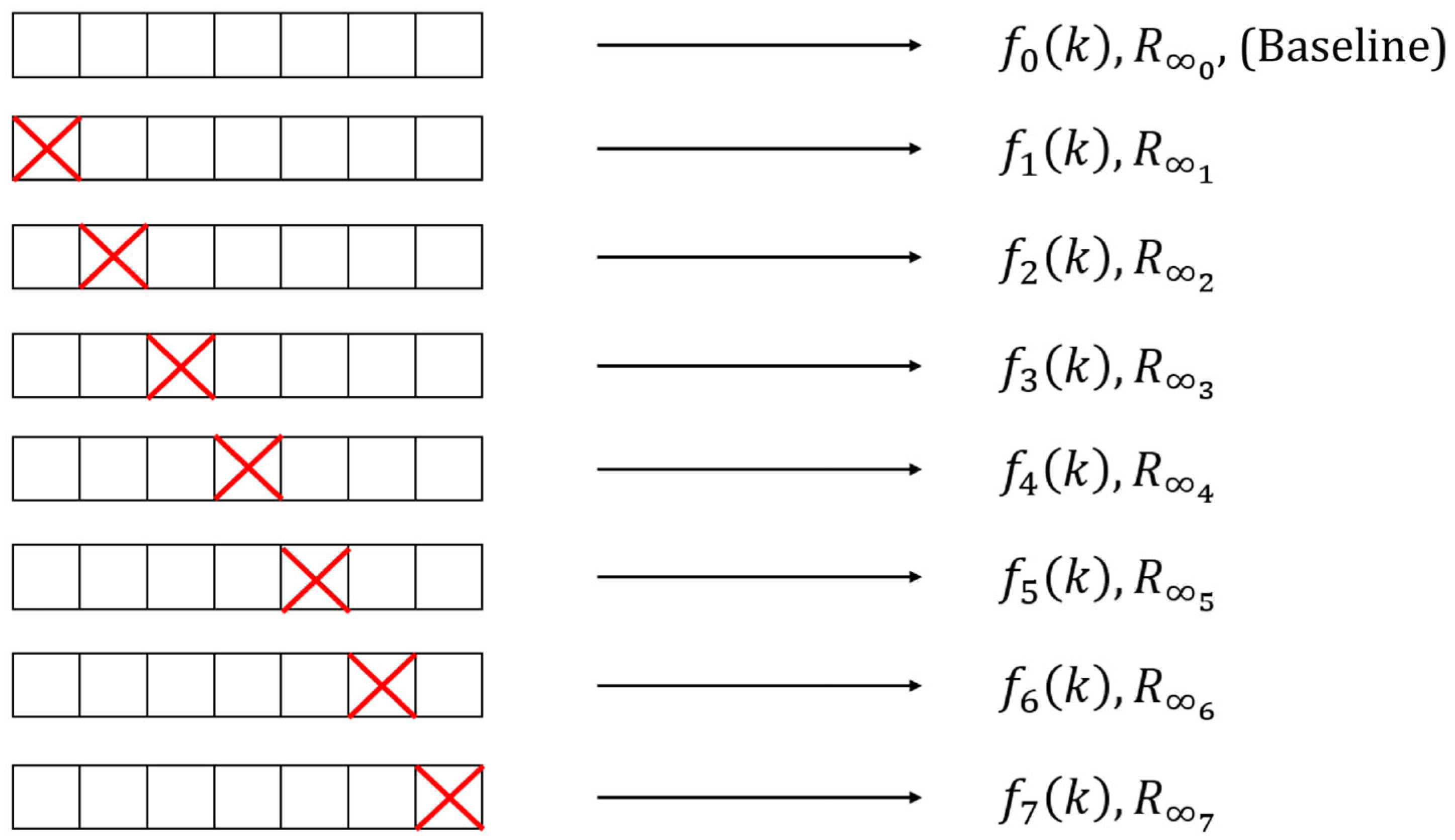
Figure 2.
Kinetic responses and model fitting in the baseline condition, with no data removal. (a) Test 1, P80 = 150 μm; (b) Test 2, P80 = 212 μm; (c) Test 3, P80 = 300 μm.
Figure 2.
Kinetic responses and model fitting in the baseline condition, with no data removal. (a) Test 1, P80 = 150 μm; (b) Test 2, P80 = 212 μm; (c) Test 3, P80 = 300 μm.
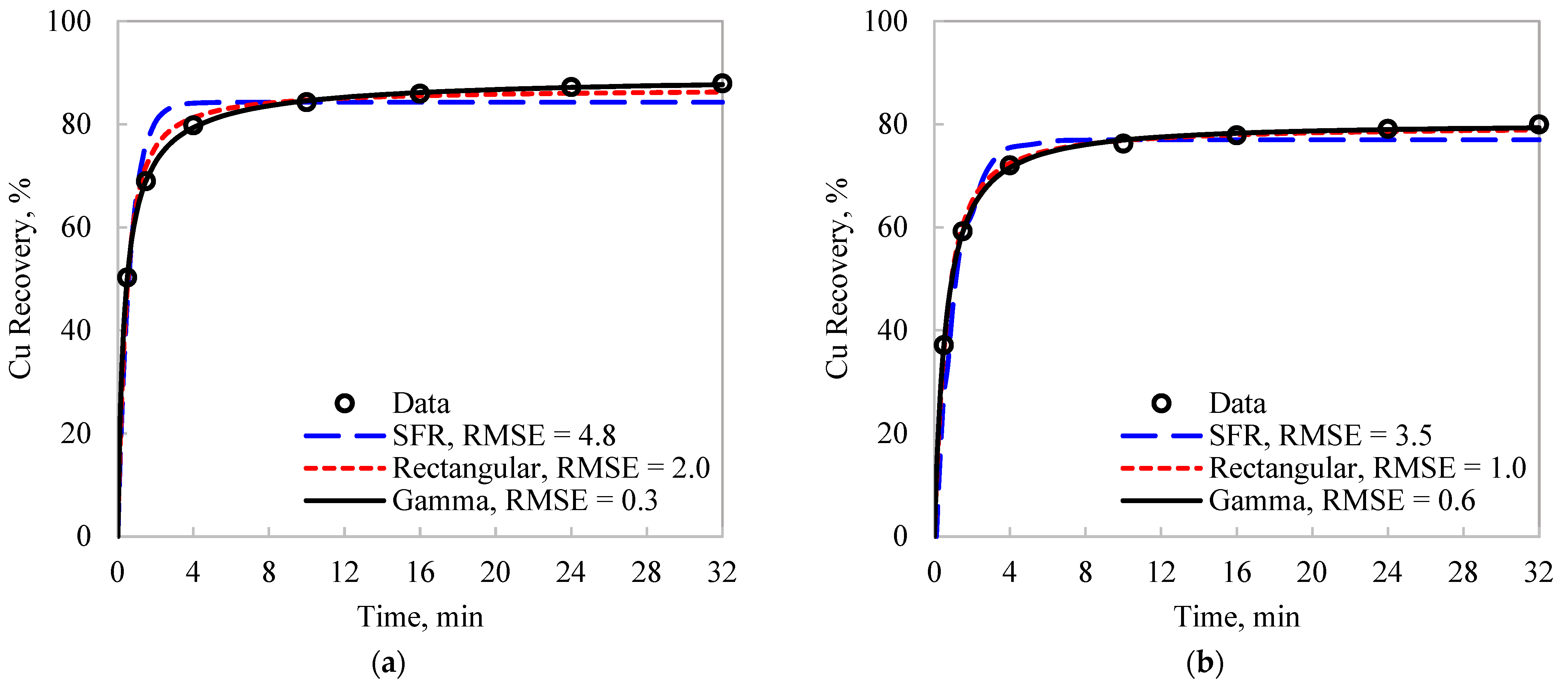
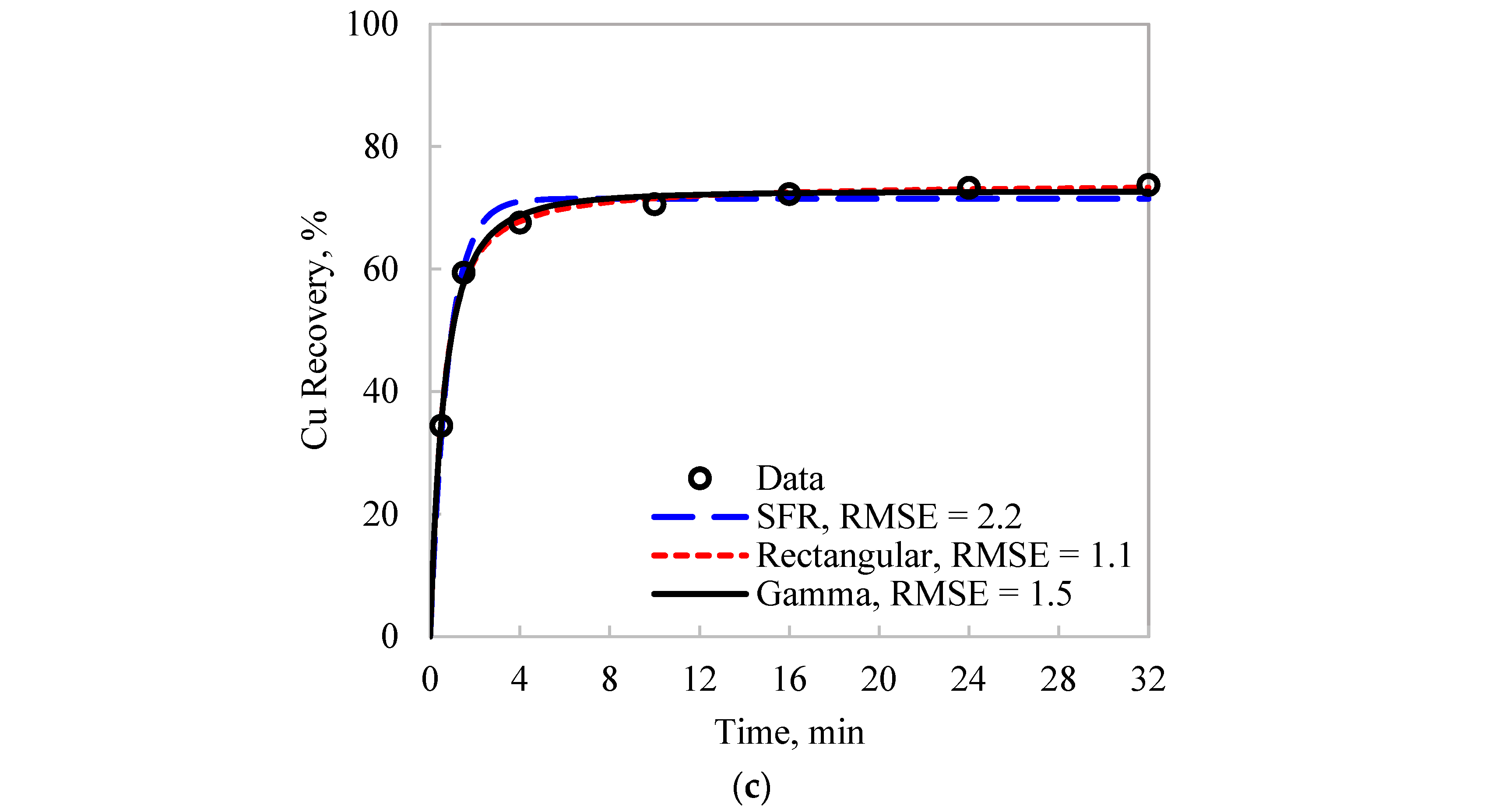
Figure 3.
Model fitting in the sensitivity analysis, Test 2 with P80 = 212 μm using the SFR model: (a) baseline with no data removal; (b) omitting the 1st datapoint; (c) omitting the 2nd datapoint; (d) omitting the 3rd datapoint; (e) omitting the 4th datapoint; (f) omitting the 5th datapoint; (g) omitting the 6th datapoint; (h) omitting the 7th datapoint.
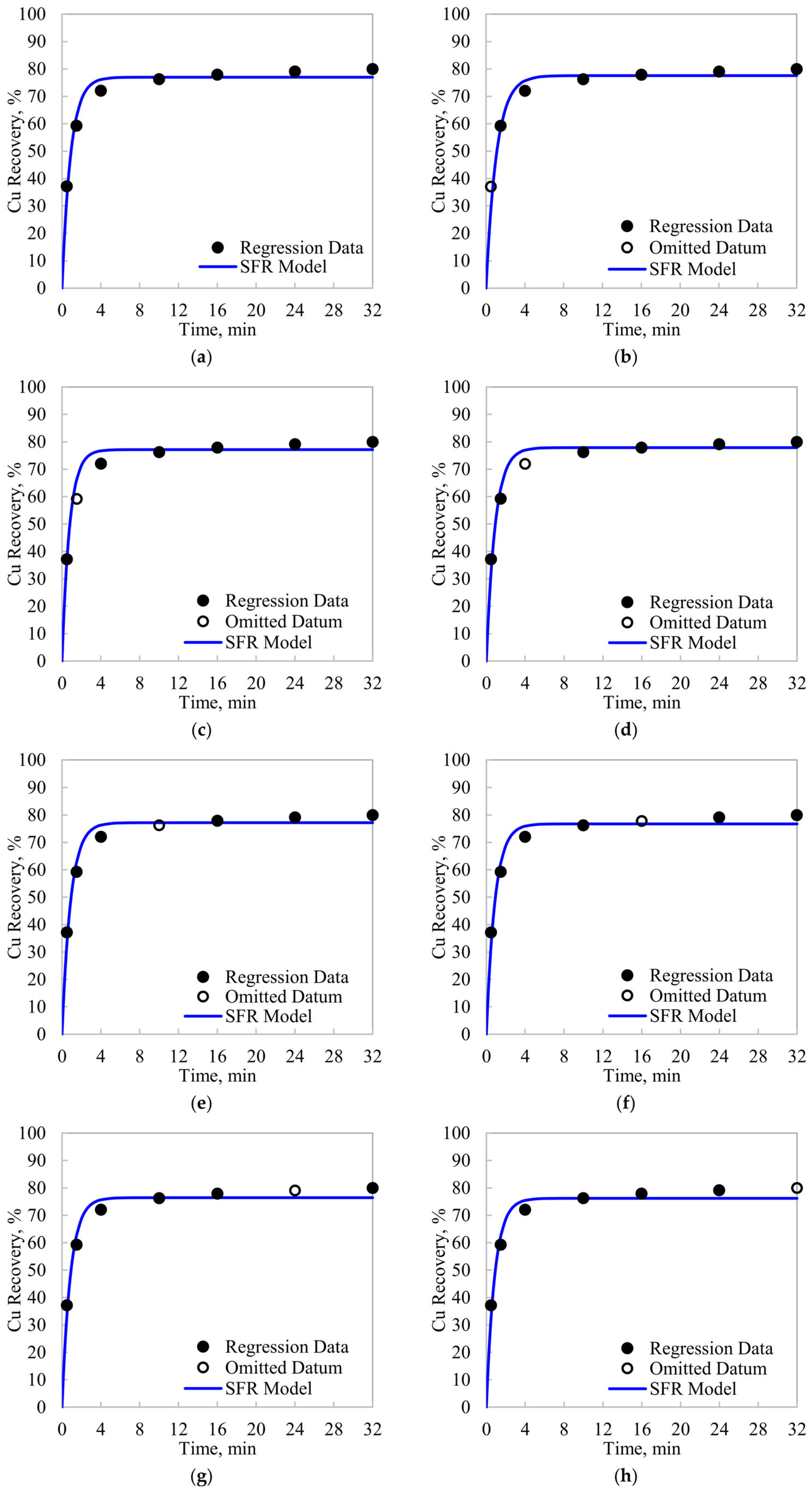
Figure 4.
Estimations of f(k), baseline and omitting one datapoint at a time: (a) Test 1, P80 = 150 µm, SFR; (b) Test 1, P80 = 150 µm, Rectangular f(k); (c) Test 1, P80 = 150 µm, Gamma f(k); (d) Test 2, P80 = 212 µm, SFR; (e) Test 2, P80 = 212 µm, Rectangular f(k); (f) Test 2, P80 = 212 µm, Gamma f(k); (g) Test 3, P80 = 300 µm, SFR; (h) Test 3, P80 = 300 µm, Rectangular f(k); (i) Test 3, P80 = 300 µm, Gamma f(k).
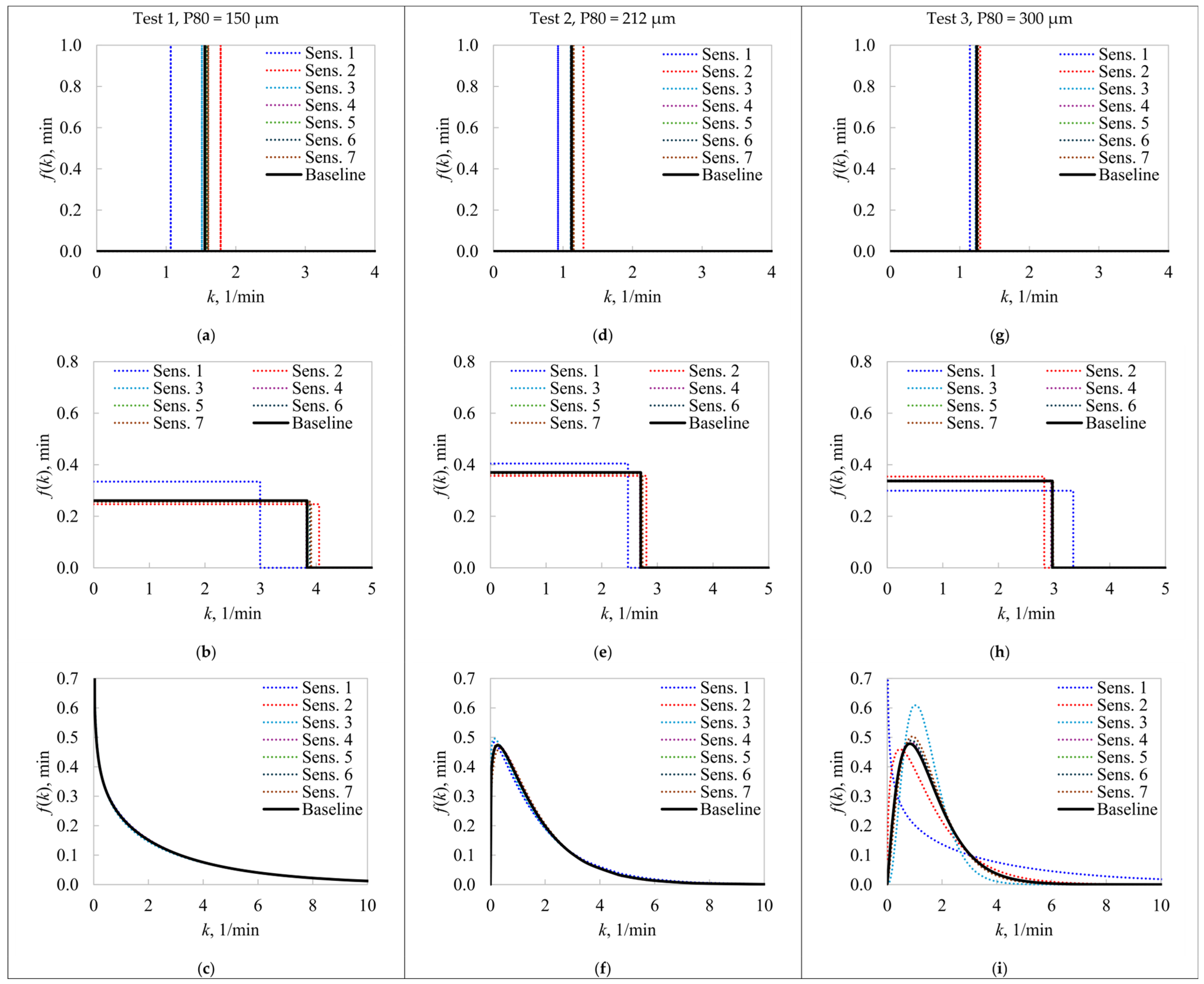
Figure 5.
Cumulative distribution functions of the R∞ estimations: (a) Test 1, P80 = 150 µm, SFR model; (b) Test 1, P80 = 150 µm, Rectangular model; (c) Test 1, P80 = 150 µm, Gamma model; (d) Test 2, P80 = 212 µm, SFR model; (e) Test 2, P80 = 212 µm, Rectangular model; (f) Test 2, P80 = 212 µm, Gamma model; (g) Test 3, P80 = 300 µm, SFR model; (h) Test 3, P80 = 300 µm, Rectangular model; (i) Test 3, P80 = 300 µm, Gamma model.
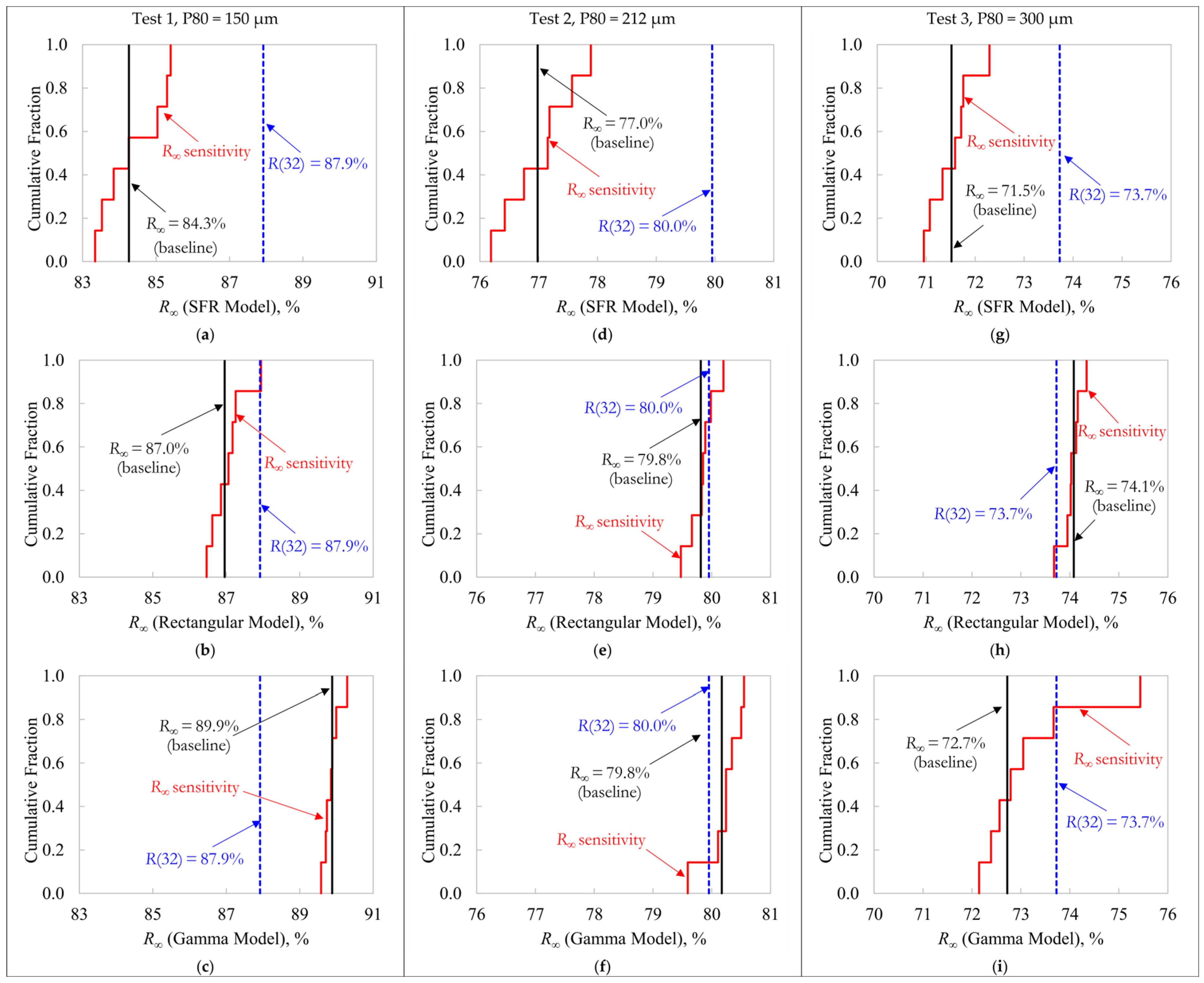
Figure 6.
Cumulative distribution functions of the scale-up recoveries at 20 min of continuous flotation, 6 perfect mixers in series: (a) Test 1, P80 = 150 µm, SFR model; (b) Test 1, P80 = 150 µm, Rectangular model; (c) Test 1, P80 = 150 µm, Gamma model; (d) Test 2, P80 = 212 µm, SFR model; (e) Test 2, P80 = 212 µm, Rectangular model; (f) Test 2, P80 = 212 µm, Gamma model; (g) Test 3, P80 = 300 µm, SFR model; (h) Test 3, P80 = 300 µm, Rectangular model; (i) Test 3, P80 = 300 µm, Gamma model.
Disclaimer/Publisher’s Note: The statements, opinions and data contained in all publications are solely those of the individual author(s) and contributor(s) and not of MDPI and/or the editor(s). MDPI and/or the editor(s) disclaim responsibility for any injury to people or property resulting from any ideas, methods, instructions or products referred to in the content. |
© 2025 by the authors. Licensee MDPI, Basel, Switzerland. This article is an open access article distributed under the terms and conditions of the Creative Commons Attribution (CC BY) license (http://creativecommons.org/licenses/by/4.0/).
Copyright: This open access article is published under a Creative Commons CC BY 4.0 license, which permit the free download, distribution, and reuse, provided that the author and preprint are cited in any reuse.


