Submitted:
27 April 2025
Posted:
28 April 2025
You are already at the latest version
Abstract
Background/Objectives: Cycling became a popular recreational sport, but it can lead to injuries and overload syndromes. The goal of this study is to evaluate the effectiveness of a training-accompanying myofascial self-massage intervention on two primary outcomes: injury occurrence and perceived training intensity. Methods: To achieve this goal we conducted a randomized controlled trial (RCT) with 35 cyclists. A difference-in-differences (DiD) regression analysis was employed to analyze the effects of the intervention. Results: The DiD analysis revealed, on the one hand, no statistically significant effect of the intervention on the overall injury score, which was observed to decrease equally in both the intervention and control groups. On the other hand, the intervention group showed a significantly smaller increase in perceived training intensity compared to the control group, supporting the hypothesis that myofascial self-massage decreases the perception of training intensity. Conclusions: The study found no evidence to support the effectiveness of a training-accompanying myofascial self-massage in reducing injury levels, but it demonstrated that the intervention may reduce perceived training intensity. Future studies with larger sample sizes and more objective injury tracking methods are needed to further explore these findings and their long-term implications for injury prevention in cycling.
Keywords:
health complaints
; symptoms of overload
; training compatibility
; myofascial self-massage
; foam rolling
; Blackroll®
; thoracolumbar fascia
; cycling
1. Introduction
With the increasing popularity of cycling as a recreational sport, health-related aspects have gained importance in recent years. Sports injuries are in most cases not caused by muscle damages but rather by injuries to the connective tissue [1], which is why experts emphasize the importance of training the fascial network as an intrinsic injury prevention mechanism, highlighting its relevance for both health as well as physical performance [2]. The fascia as a metasystem is the only system that connects and influences all physiological functions of the body [3]. As empirical evidence suggests, the fasciae play a significant role in proprioception and serve as the primary site of interoception [4]. Rather than exerting force directly on their bony insertions, most muscles transmit a substantial part of their force laterally to adjacent muscles and other structures via myofascial force transmission. Moreover, the interconnected fascial network within muscles likely plays a role in regulating and adapting muscle mass through mechanical and biomechanical signaling [5].
Several factors can contribute to a dysfunctional fascial system, including a lack of movement, poor posture, imbalanced loading, incorrect or excessive strain or overly intense training, which can ultimately lead to muscle pain, tension or movement restrictions [6]. Within the context of cycling the long fascial line of the posterior chain can experience uneven stress: the calves, thighs and hips typically operate in small ranges of motions for extended periods, often leading to shortening of the hamstrings, while the entire back remains continuously stretched due to the forward-leaning seated position on the bike. Furthermore, structures above the knee and at the hip often show reduced mobility. Unevenly trained structures can also lead to fluid retention in the muscular connective tissue, which may restrict the entire muscle-fascia unit – a problem that can shorten the muscle fibers [7].
Given these characteristics and implications of the connective tissue, it is reasonable to integrate a specific fascial training into personal and athletic training routines. According to Müller and Schleip, the goals of fascia training include the stimulation and activation of fibroblasts to dissolve cross-links, adhesions or myofascial trigger points, thereby restoring the original wave-like structure with a crisscross fiber arrangement, which is often compromised by aging or inactivity [2]. Short, regular and long-term (six months to two years) fascia training has been shown to improve movement patterns and coordination, which results in more efficient muscle function, enhanced body awareness, injury prevention, faster recovery times or an improved overall performance [2,7]. In many cases stretching, massage or other non-invasive rehabilitation tools and techniques are not enough to relax the ITB [8]. To achieve these benefits athletes can apply various release techniques, such as myofascial release or self-myofascial release using foam rollers [9]. Foam rollers are used for self-myofascial release, which is supposed to be an effective intervention for preventing injuries and overload syndromes, such as the iliotibial band (ITB) friction syndrome [8].
In addition to injury prevention and reduction, foam rollers are often associated with factors related to athletic performance and training intensity. For instance, the application of self-myofascial release techniques correlates with an increased range in motion and higher flexibility [10,11]. Other studies show empirical evidence that self-myofascial massage might reduce muscle fatigue and, therefore, enhance athletic performance during training. It is theorized that self-myofascial release increase muscle blood volume, which might help to remove lactic acids [12]. Reduced muscle fatigue, self-myofascial release may contribute to the perception of athletes that they can work out harder and longer [13].
The following study analyzes the potential impact of training-accompanying myofascial self-massage on health, injuries and overload syndromes, on the one hand, and on the perceived training intensity, on the other. To achieve this goal, the author conducted an exploratory longitudinal randomized controlled trial (RCT) analyzing the long-term effects of a six-month intervention involving training-accompanying myofascial self-massage in the lower extremities and the Fascia thoracolumbalis. For the myofascial self-massage the Blackroll® was applied twice a week, immediately following a cycling training session.
The analysis of the training-accompanying myofascial self-massage in the following study focuses on two primary goals: (1) the impact on the frequency of health complaints and overuse symptoms and (2) the impact on training tolerance and perceived training intensity. To answer these questions the study uses a difference in differences (DiD) regression analysis [14].
2. Theoretical Background and Hypothesis
This study investigates training-accompanying myofascial self-massage using the Blackroll® as the independent variable and its impact on various dependent variables. The Blackroll® is a foam roller used in various exercises to increase the elasticity and performance of the muscles and the fascial tissue [15]. During the trial preparation phase the participants received detailed instructions on how to apply the Blackroll®. With the begin of the intervention phase the participants were required to follow a specific training program consisting of twelve exercises, which target different body parts and tissues, as recommended by the manufacturer. These exercises focused on the plantar fascia, calf, tibialis anterior, quadriceps, hamstring, adductors, iliotibial band, psoas, gluteal muscle, lower back as well as upper back [16,17]. The application of the Blackroll® was performed twice a week immediately after a cycling training session for a duration of six months. The participants were not allowed to conduct additional accompanying measures such as massages or other self-massages.
Whereas the intervention serves as the main independent variable, we will test two different main dependent variables. The first main dependent variable will be the overall level of injuries and overload syndromes, which will be measured by a score that combines the number of injuries, the frequency of the injuries, the timing of the injuries as well as the intensity of the injuries. To analyze the impact of the intervention on the overall level of injuries and overload syndromes will be tested with the following main hypothesis:
H1:
The application of training-accompanying myofascial self-massage of the fasciae using the Blackroll® leads to a reduction in health complaints and overuse syndromes related to cycling.
While the hypothesis H1 investigates the level of injuries and overuse syndromes, the study also includes an analysis of the impact of the intervention on the subjective perception of the training intensity. Based on the findings of various studies [10,11,12,13] we theorize that the intervention results in a decreasing perception of the training intensity. To test the impact of the intervention on the perceived training intensity we formulate the following hypothesis:
H2:
The application of the training-accompanying myofascial self-massage of the fasciae using the Blackroll® results in a decreasing perception of training intensity.
In addition to the intervention as the primary independent variable, the analysis will test a range of hypotheses that account for additional control variables that may influence the target variables. These variables include physical characteristics such as age, weight or BMI as well training-related factors such as the type of bicycle used by participants.
H3:
There are correlations between age and the target variables. The higher the age, the more severe and frequent complaints and overload syndromes occur and the higher the perceived training intensity.
H4:
There are correlations between BMI and weight and the target variables. The higher the BMI and weight, the more severe and frequent complaints and overload syndromes occur and the higher the perceived training intensity.
H5:
There are correlations between the type of bicycle used by participants and the target variables.
3. Study Design and Data
3.1. Study Design
To examine the impact of the Blackroll® on the health of cyclists and overuse syndromes, this study employed an exploratory, longitudinal randomized controlled trial (RCT). RCTs are widely considered the gold standard for assessing the causal effects of an intervention or a treatment [18]. The intervention in the following analysis involved a regular training-accompanying myofascial self-massage of the fasciae using the Blackroll® twice a week in the lower extremities and the Fascia thoracolumbalis immediately after cycling training. The participants were randomly divided into an intervention group, which integrated the Blackroll® into their training program, and a control group, which participated in the trial and continued regular cycling training but without using the Blackroll®.
Another key feature of RCTs is that data is collected at multiple points in time [19]. According to the scholarly literature, fascial structures adapt slowly. To achieve positive and lasting effects, regular long-term fascial training – over a period of six months to two years – is recommended, which involves a short exercise program lasting only a few minutes per session. The fibroblasts stimulated in the connective tissue initially increase their collagen degradation activity within the first one to two days, after which collagen synthesis becomes predominant. Therefore, fascial training should ideally be performed once or twice per week [20]. For this study the intervention phase lasted six months, in which the study began with a baseline measurement prior to the intervention, followed by two follow-up measurements during and after the intervention period (first post-test, second post-test). The first post-test took place three months after the trail had started and the second post-test three months after the first post-test.
3.2. Data Collection
This study focuses on adult recreational cyclists as the target population. Participants were selected by the author based on a number of the inclusion and exclusion criteria. Despite extensive efforts, only three female cyclists could be recruited, so the study was ultimately conducted with only male cyclists. Originally, we recruited 36 cyclists, however, one participant dropped out during the trial. Therefore, the total sample size (N) consists of 35 male recreational cyclists, which were divided into two groups, 18 in the intervention group and 17 in the control group. All participants had a comparable baseline level, with an average training volume of 8 to 10 hours per week and a minimum of three years of cycling-specific training experience. The age range of participants was between 26 and 56 years at the time of the trial. The study was conducted in cooperation with cycling clubs across Tyrol, Austria. Recruitment was carried out through a written email distributed to all cycling clubs and lasted from mid-March to mid-September.
To be eligible for the study, participants had to meet the following criteria:
- Age between 20 and 56 years at the time of the baseline test
- Active recreational cyclist
- Average training volume of 8 to 10 hours per week
- At least three years of cycling-specific training experience
- A spiroergometry test performed within the last two years
- Pulse-controlled training for the past three years
- No training interruptions longer than six weeks in the past three years
- A medical health certificate, issued within the last two months, confirming no contraindications or risks associated with maximal exertion until exhaustion
In addition to the inclusion criteria, participants were excluded from the study if they met any of the following conditions:
- Licensed competitive cyclists
- Individuals diagnosed with osteoporosis, disc damage, thrombosis, high blood pressure (above a specific threshold), fibromyalgia, or soft tissue rheumatism
- Individuals with a knee or hip joint implant
- Participants who develop acute or chronic illnesses during the study
Participants were excluded from the analysis if they dropped out, as no intent-to-treat analysis was conducted. The discontinuation criteria were categorized as follows:
- Study dropouts: Individuals, who voluntarily withdrew from the study, were not included in the evaluation.
- Intervention-related events: This included adverse events, intercurrent illnesses or failure to adhere to the training protocol.
- Non-intervention-related events: This included withdrawal of consent or the discovery of exclusion criteria after the study had begun.
Participants in the intervention group followed a structured precisely defined, pulse-controlled 80-minute cycling training session twice per week. Training was conducted in the G1 and G1/G2 intensity zones and included strength-endurance intervals. Additionally, they performed a standardized myofascial self-massage of the fasciae of the lower and upper extremities and the thoracolumbar fascia using the Blackroll®, immediately after each cycling session. Participants in the control group also completed a precisely defined, pulse-controlled 80-minute cycling training session twice per week, like the intervention group. However, their training occurred in the aerobic-anaerobic transition zone (with lactate levels between 2 and 4 mmol/l) and included the same strength-endurance intervals as the intervention group. The control group was instructed to follow the same cycling training as participants in the intervention group, but without applying the Blackroll®.
During the tests the training and measurements followed a highly controlled protocol. First of all, the tests were conducted on the participants’ own race bicycle, starting with 100 watt and a 50 watt increase every three minutes. Moreover, the training was heart rate-controlled and took place indoors. The spiroergometry and lactate measurements were conducted with the CYCLUS 2. Spiroergometry and lactate measurement using the CYCLUS 2 on the participants’ own racing bike allowed us in this context to determine heart rate zones for training control. The aerobic and anaerobic thresholds were determined according to Mader A. at 2 and 4 mmol/l. During the tests we independently measured power meter pedals with the Vector2™, along with a compatible Edge® bike computer, both of which from Garmin®. This means that both pedals were equipped with measurement electronics, which allowed us to measure the power output and force distribution separately for each leg.
Both groups completed a precisely structured, 80-minute heart rate-controlled cycling session twice per week in the aerobic zone (basic endurance 1, GA1) and basic endurance 2, GA2), with lactate levels between 2 and 4 mmol/l) at a cadence of 90 to 100 revolutions per minute (RPM). After a 10-minute warm-up in the lower GA1 range, the session continues with 3- to 5-minute extensive strength endurance intervals (KA intervals) in the GA2 range at 60 to 70 RPM. These intervals were performed with a 1:1 ratio of interval to recovery, with the recovery taking place in the GA1 range at 90 to 100 RPM.
Additionally, we implemented the training based on a so-called block periodization with a total number of six blocks, each of which lasting four weeks. After each block training intensity was increased by 5%, based on the individual performance at 2 mmol/l determined during the baseline test. Each training session was fully recorded, including the heart rate, wattage and cadence, and subsequently documented in terms of training intensity to ensure that all parameters were strictly followed. The study also utilized block randomization (4x4). A randomization list was managed by the project leadership, who assigned participants to either the intervention or control group based on this list once the author of this study obtained their informed consent.
The intervention phase followed a structured plan for recreational cyclists designed by the author, based on many years of experience as a state-certified trainer, a teaching qualification for movement and sport and former successful cyclist at national and international level. Before the study began, a three-week preparatory phase ensured that participants received detailed personal instructions on how to properly execute the training protocol. Furthermore, the author conducted pretests prior to the intervention phase to validate and test the data collection process and prevent potential measurement errors. The pretest involved twelve amateur cyclists within the context of a seminar, during which we tested our setup and measurement protocols. The recruitment of the participants, instructions and pretests took place in September (week 37-40), followed by the baseline test in early October (week 41-42). The intervention began mid-October (week 43) and lasted 24 weeks, during which participants completed two precisely defined, pulse-controlled cycling training sessions per week, each lasting 80 minutes within the aerobic-anaerobic transition zone, at intensities that result in a lactate concentration of 2 to 4 mmol/l. Both the intervention and control groups followed this trainings with strength-endurance intervals of four weeks each. After three months we conducted the first post-test and after six months the second post-test. In addition, a food diary was kept throughout the entire period.

Table 1.
Time schedule for the data collection process during the preparation and intervention phases (Source: own illustration).
Table 1.
Time schedule for the data collection process during the preparation and intervention phases (Source: own illustration).
| Month/Week | Milestones and data collection |
|---|---|
| March-September (week 12-38) | Recruitment of participants |
| September (week 39) | Detailed instructions for participants |
| September (week 40) | Pretests |
| October (week 41-42) | Baseline tests |
| October (week 43) | Beginning of intervention phase |
| January (week 1) | 1st post-test for intervention group |
| January (week 2) | 1st post-test for control group |
| March (week 13) | 2nd post-test for intervention group |
| April (week 14-15) | 2nd post-test for control group |
| April (week 15) | End of intervention phase |
3.3. Operationalization of the Variables
The health complaints and overload syndromes, which represent the dependent variables in H1, were measured by a standardized questionnaire, assessing the subjective perception of various health complaints and overload syndromes. The questions and attributes used to assess the complaints and overuse syndromes were partially derived from Tofaute [21], a study conducted by the Cologne Sports University. Furthermore, the conceptualization of this project was combined with survey designs developed by Kromer et al. [22] and Froböse et al. [23]. The same questionnaire was used for all tests, including the baseline test before the intervention phase, the first post-test and second post-test, which marked the end of the trial for the participants. The assessment of the health complaints and overuse syndromes consists of various sections, including questions on (1) the localization and frequency of the complaint, (2) the type of the complaint, (3) the point in time of the complaint and (4) the intensity of the complaint.
The various health complaints and overuse syndromes were assessed for different localizations and body parts, including finger and finger joints, wrists, arms, shoulders, neck and cervical spine, lower back and lumbar spine, gluteal, hip joint, upper legs, knee, feet and toes or other complaints. To assess the frequency of complaints, participants were able to choose between rarely and frequently. No response indicated that the participant did not experience any health complaints or overload injuries. In addition to the localization of the complaint, the questionnaire asked for the type of complaint, including pain, tensions, convulsion, formication, numbness, stiffness and skin problems. Regarding the timing of the complaint, the survey asked whether the complaint occurred during or after the cycling training or both. The question about the intensity of the complaint included three attributes: tolerable, disturbing and intolerable.
For the statistical analysis of H1, which tests the overall level of complaints, injuries and overload syndromes, we calculated a factor variable based on a cumulative score, which combines all body parts and attributes, consisting of (1) the total number of complaints (1 point per injury or complaint, 2 points for two complaints, etc.), (2) the frequency of complaints (0 point for no occurrences, 1 point for rare occurrences and 2 points for frequent occurrences), (3) the timing of the complaint (0 point for no complaints at all, 1 point for during the training, 1 point for after the training and 2 points for both) and (4) the intensity of the complaint (1 point for tolerable, 2 points for disturbing and 3 points for intolerable). In sum, we calculated a metric variable with a score that combines different factors and represents the overall level of injuries and complaints. Scores were calculated for each specific body part, with higher scores indicating more severe injuries and complaints.
H2 examines the impact of the application of the Blackroll® on the perception of the training intensity. Perceived training intensity was measured using the 10-point version of the RPE scale, ranging from 0 (nothing at all) to 10 (extremely strong), which has shown reliability and validity especially when used among healthy, clinical and athletic adult populations [24]. Finally, H3-H5 investigate the correlation between generic physical indicators as independent control variables, on the one hand, and the level of injuries and the perceived training intensity as dependent variables, on the other. The generic physical indicators included questions about the age, body weight and body height. Finally, the survey collected generic data related to the cycling training, such as the type of bike used by participants and their annual relative distribution or whether and how often participants engaged in compensatory training.
3.4. Data and Structure of Dataset
This leads us to the characteristics of the data and the structure of the dataset. The questionnaires and measurements were conducted during the baseline test, first post-test and second post-test. For the final dataset one participant was excluded for violating the inclusion criteria. As a result, the dataset includes data for 35 recreational cyclists, of whom 18 were in the intervention group and 17 in the control group. Due to the measurements and the structure of the questionnaire, the final dataset contains 244 different variables.
The first cluster of variables provides physical and demographic data, such as age group, body weight, body height, BMI or group assignment (intervention or control group). Another set of variables includes data on cycle training, such as different types of bicycles and their relative distribution in percentages or the frequency of compensatory training. A third cluster of variables focuses on injuries and complaints affecting different body parts, including fingers, wrists, arms, shoulders, neck and cervical spine, lower back and lumbar spine, gluteal, hip joint, upper legs, knee, feet and toes as well as other complaints. For each body part, the dataset provides information on the frequency of complaints, type of complaint, intensity of the complaint and whether the complaint occurred during and after the cycling or both. For the second main dependent variable, the dataset includes an ordinal scaled variable between 0 and 10 measuring subjective and perceived training intensity. In addition to cross-sectional data, the dataset includes longitudinal data for each of these clusters, with three data points collected during the baseline test, first post-test and second post-test.
Table 2.
Most important variables and structure of dataset (Source: own illustration).
| Variable | Description |
|---|---|
| Group | Categorical variable with the attributes intervention or control group |
| Age group | Interval scaled variable with four age groups: 20-30, 31-40, 41-50 and 51-60 years |
| Body weight | Metric variable measured in kg |
| Body height | Metric variable measured in cm |
| BMI | Body Mass Index is calculated by weight in kg divided by the square of the height in m. |
| Compensatory training | Semi-metric variable, frequency of the compensatory training with the attributes once, twice, three or more times a week or none. |
| Cycle type racing bicycle | Metric variable in % relative to other types |
| Cycle type mountain bike | Metric variable in % relative to other types |
| Cycle type indoor | Metric variable in % relative to other types |
| Cycle type other | Metric variable in % relative to other types |
| Complaint frequency* | Categorical variable with the attributes rarely and frequently |
| Complaint type* | Categorical variable with the attributes pain, spasms, numbness, skin problems, tension, formication, stiffness, multiple answers were possible |
| Complaint time* | Nominal scaled variable with the attributes during cycling, after cycling training or both |
| Complaint intensity* | Ordinal scaled variable with the attributes tolerable, disturbing and intolerable |
| Perceived training intensity | Ordinal scaled variable with a scale from 0 to 10 with 10 being the highest perceived training intensity |
* The variables frequency, type, time and intensity were measured for several body parts, which are not displayed in the table, including fingers, wrists, arms, shoulders, neck and cervical spine, lower back and lumbar spine, gluteal, hip joint, upper legs, knee, feet and toes or other complaints. ** The variables score before, score after and score difference were measured and calculated for multiple body areas, including upper limbs, lower limbs, back and buttocks. Note that the variables in the table are available for multiple points in time (baseline test, first post-test, second post-test).
4. Statistical Methods
Before the study analyzes the different hypotheses, the first step of the statistical analysis is to provide a general overview and frequency distributions of the most important variables using methods from descriptive statistics. This includes frequency statistics, averages and graphical representations illustrating the distribution of key variables and their attributes. Part of the descriptive analysis is the characterization of the sample. Another part is a correlation analysis, which investigates the relationships between the variables. The main goal of the correlation analysis is to get an overview of bivariate relationships. Another goal of the correlation analysis is to check whether the independent variables correlate with each other to avoid multicollinearity. To conduct the correlation analyses we used Spearman correlations.
In the second step of the statistical analysis, we used methods from inferential statistics. One of the most important goals of randomized controlled studies with an intervention group and a control group, measured at multiple points in time, is to analyze the causal effects of an intervention using statistical methods. One such method used for analyzing causal impacts is the difference-in-differences (DiD) regression model, which has become a popular approach for intervention analysis [25]. DiD analysis can be applied in cases where the outcome of a specific intervention in a treatment or intervention group is analyzed and compared with a control group both before and after a treatment or intervention takes place [26]. In a simple DiD regression analysis we control for the time and group and focus on the interaction term, which includes both time and group. The two differences in the DiD model represent, on the one hand, the difference in the means of the response variable between the intervention group and the control group after the treatment and, on the other hand, the difference in the means between the intervention group and the control group before the treatment [22]. By calculating the difference-in-differences we obtain the so-called treatment effect or DiD estimator δ, which can be expressed by the following formula:
where represents the mean of the treatment gorup after the intervention, the mean of the control group after the intervention, the mean of the intervention group before the intervention and the mean of the control group before the intervention.
In the following analysis the DiD estimator will be integrated into a DiD regression model, which has the advantage that additional factors or covariates can be integrated and controlled. The DiD regression model consists of indicator variables for the intervention before and after the treatment as well as their interaction term. Note that in the DiD regression model the coefficient δ on the interaction term exactly represents the DiD estimator in formula (1) [27]. In its simplest implementation the DiD regression model can be defined by the regression formula
in which represents the response variable, is the baseline value before the intervention started and is applied to the control group – in the regression model the intercept, captures the effect of time on the outcome variable, which affects both groups equally and is a time dummy variable with a value of before the intervention and after the intervention. is a treatment group dummy variable with for the control group and for the treatment group, whereas reflects the pre-existing differences between the treatment and control groups before the intervention. The interaction term represents the treatment effect, measuring the causal impact of the intervention by comparing how the treatment group changes relative to the control group or how many more units one group changed compared to the reference group. The interaction is what makes the DiD regression model different from a simple before-after comparison, as it accounts for any general time trends that affect both groups. Finally, represents the error term, which includes all unobservered factors that might influence the response variable.
Since the analysis includes additional variables, which will be tested as covariates, the regression formula can be extended by incorporating control variables and and their respective coefficients and :
A specific feature of general DiD models is that they only consist of the two time periods before and after. Since the data in the following analysis includes three time periods, the DiD regression analysis in this study requires a specific two-part procedure. In the first part, conventional DiD regression models with two time periods will be conducted, using the DiD regression formulas (2) and (3). This includes
- Differences between the baseline test (before the start of the intervention) and the second post-test (end of the trial),
- Differences between the baseline test (before the start of the intervention) and the first post-test (end of the first intervention phase) and
- Differences between the first post-test (end of the first intervention phase) and the second post-test (end of the trial).
Comparing the individual DiD regression models provides the opportunity for a more fine-grained analysis of the progress during the trial. In the second part, a dynamic regression model will be tested, incorporating a baseline test and two post-tests. DiD regression models, which extend beyond the conventional 2x2 setting, include separate treatment effects for each post-intervention period, which can be expressed by the following regression formula:
where represents the response variable, is the intercept of the regression line with the y-axis, which is in this case the baseline outcome, reflects the time effect, which captures the trends over time, is the group effect, which represents the baseline differences between the intervention and control groups. The term defines the dynamic treatment effects, in which the term are dummy variables for different post-treatment periods, stands for the treatment effect at different points in time. The part of the formula in represents the additional control variables and their coefficients and the is the error term that accounts for the influence of other factors. The regression models were derived and adjusted based on the descriptions in [25,26,27]. SPSS 25.0 and Python 3.9 were used to perform the statistical analyses.
5. Results
In the following section we present the experimental results, their interpretation and the conclusions derived from the data, which consists of two subsections. In the first subsection we provide a general overview of the sample and the most important variables, using methods from descriptive statistics. In the second section we analyze the hypotheses based on the DiD regression models.
5.1. Descriptive Analysis of the Participants’ Basic Physical Characteristics
The descriptive analysis of the sample reveals the basic characteristics of the participants and the main variables. The data appears to be skewed toward the middle age groups, with the highest frequency occurring in the 41–50 category (18 participants), followed by the 31–40 category (11 participants). The 20–30 (1 participant) and 51–60 age groups (5 participants) have significantly lower frequencies, indicating that most participants fall within the middle age ranges. This suggests that the sample is not evenly distributed across age groups and is concentrated in the 31–50 range. The most notable observation is that both groups have the same peak in the 41–50 age category. However, there are some differences in the distribution of the categories. The intervention group has a higher frequency in the 31–40 category compared to the control group, suggesting that slightly younger participants were more likely to be assigned to choose the intervention. In contrast, the control group is more evenly spread across the older categories, particularly in the 51–60 range. The 20–30 age category has the lowest representation in both groups, which means that younger participants are underrepresented.
Several differences can be observed in the distribution of BMI classes for the intervention and control groups. Most participants in both groups fall within the 21–25 BMI range, indicating that most individuals have a normal BMI. However, there is a noticeable peak in the normal weight category for the control group, where its frequency is higher than in the intervention group. In contrast, the intervention group has a higher representation in the overweight class. This suggests that the intervention group includes individuals with a slightly broader range of BMI values, potentially influencing the results if BMI plays a role in the intervention outcomes. The absence of participants in the extreme BMI categories (<19 or >31) in both groups indicates that most individuals fall within a moderate range, which could be beneficial for the comparability of the two groups. In the overall sample the participants have on average a BMI of 23.85, with a minimum of 19.49, a maximum of 29.7 and standard deviation of 2.3. Given these differences in both groups and their potential impact on health complaints, it is reasonable to consider the BMI as control variable in the regression models.
5.2. Descriptive Analysis of Health Complaints and Their Frequencies
Before we dive deeper into the analysis and investigate the impact of the intervention on health complaints using DiD regression analysis, the following section presents a descriptive overview of the different health complaints and overuse syndromes for the intervention and control group. Table 3 below shows the share of participants (in % of their group) and the total number of individuals, who reported a health complaint for each specific body part at the baseline test (before the intervention started). There are a couple of interesting insights that can be drawn from the descriptive analysis of the number of injuries and complaints, one of which is that a relatively high number of individuals in both groups reported health complaints in regard to their spine – a fact that is consistent with various studies indicating negative health outcomes of cycling for the spine [28,29,30]. A notable difference between the intervention and control group when it comes to spine problems is that the intervention group shows a high amount of neck/cervical spine problems (44 %), while the control group reported a higher number of individuals with lumbar spine complaints (29.4 %). In the overall sample 60 % of the participants either reported problems with the neck and cervical spine or the lumbar spine.
Another body part, which is associated with a significant number of health complaints, is the knee with an overall share of 34.3 % of the individuals, who reported knee problems before the intervention started. Both groups reported the same total number of complaints regarding the knee. Like the spine complaints, this result is also consistent with the academic literature, in which knee problems are often considered as one of the most common negative health outcomes among cyclists [28,31]. As can be seen in Table 3, spine and knee problems are followed by complaints regarding the fingers (7 complaints), the wrists (7), upper legs (6), gluteal (5), shoulders (5), hip joint (4), feet/toes (4), other complaints (4) and arms (2). Finally, it should be mentioned that both groups showed a similar number of injuries, with a total number of 40 complaints in the intervention group and 37 complaints in the control group.
5.3. Descriptive Analysis of the Overall Score of Complaints and Injuries
The following section includes a descriptive analysis of the scores that represent the overall level of injury for each body part. In contrast to Table 3, which contains the total number of injuries and complaints at the baseline test, the scores in Table 4 and Table 5 are calculated based on the frequency and intensity of the injury for each body part. Like the ranking in Table 3, the highest score occurred for the neck/cervical spine in the intervention group with total score of 45, followed by knee injuries with a total score of 33 in the control group and a score of 32 in the intervention group. Although most body parts show a similar level of injuries in both groups, there are a few body parts with major differences between the two groups, one of which is the neck/cervical spine. Another major difference between the two groups can be observed at the hip joints with a score of 21 in the intervention group and a score of 3 in the control group.
Whereas in most cases the ranking of the scores correlates with the absolute number of injuries, the gluteal complaints rank higher in Table 4 than in Table 3, which could mean that the complaints related to the gluteal tend to be more severe and frequent. As can be seen in the sum of Table 4, the intervention group showed a higher overall score with 223 points compared to 187 points in the control group, which can be partially explained by the fact that the intervention group had a slightly higher total number of injuries and complaints.
Table 5 shows, on the one hand, the scores for each body part and each group in absolute terms at the first post-test and the second post-test and, on the other hand, the changes in the score compared to the previous test. As can be seen in the table below, the biggest change occurred for the neck/cervical spine in the intervention group with a total reduction of 30 score points, followed by the lumbar spine in the control group with a decrease of 18 score points. The most significant changes occurred in both groups after three months in the trial (first post-test) with a total reduction of 105 score points in the intervention group and 78 score points in the control group. The intervention group also showed a greater reduction in the overall injury level at the second post-test compared to the control group, even though the changes were significantly lower than the changes at the first post-test. In other words, the intervention group showed a slightly greater reduction in the overall injury level than the control group at the first and second post-test, which could mean that the application of the Blackroll® may have a slight impact. However, the difference in the average change per participant between the intervention and control group is very minimal because the control group also showed a significant reduction in their overall score, which means that other influential factors might have to be considered as well – some of those potential factors will be analyzed as part of the correlation analysis and regression models.
5.4. Correlation Analysis of the Main Variables
As part of the correlation analysis, we first investigate the first main variable: the overall injury score, which reflects the number of injuries and complaints and their extent and severity. The overall score shows only one statistically significant correlation in the dataset, which is a moderate, negative correlation with the variable bicycle type mountain bike (r = -0.37, p < 0.05). This may suggest that individuals, who primarily use a mountain bike, tend to report fewer overall complaints or injuries. Theoretically, it is possible that mountain bikers engage in more varied and technically demanding riding styles that promote physical resilience. Another explanation would be that mountain bikers are less likely to injure their spine due to their position on the bike, which differs from the position of racing bikers. Regarding the anthropometric variables such as BMI, body weight or age we originally expected a higher BMI or older age to be associated with a higher level of injury and complaints, but the correlation analysis does not support this assumption.
The second main variable is the subjective intensity of the training, for which we can observe several significant correlations. The strongest correlation can be observed between the intensity and body weight (r = 0.71, p < 0.01), whereas the BMI (r = 0.37, p < 0.05) and height (r = 0.45, p < 0.01) show moderate correlation with intensity, indicating that heavier and taller individuals also show higher intensity levels. The strong correlation between intensity and body weight suggests that individuals, who weigh more may perceive their training more intensively. Contrary to what we originally assumed, we did not find a significant correlation between the intensity and the overall score, which suggests that the perceived intensity of physical activity is not directly related to more or fewer complaints. Similarly, we did not observe a significant relationship between the perceived training intensity and age – another assumption that was rejected by the correlation analysis.
Furthermore, body weight and BMI are strongly correlated (r = 0.71, p < 0.01), which is to be expected given that BMI is derived from weight and height. Weight also correlates significantly with height (r = 0.56, p < 0.01), indicating that taller individuals naturally tend to have a higher weight. These internal consistencies support the reliability of the data. However, neither BMI nor weight is significantly correlated with the overall score, even though it could be assumed that individuals with higher BMI might be at greater risk of musculoskeletal complaints.
Regarding the variable age, we could not find any significant correlations with the overall score or perceived intensity. One of the interesting findings here is that age shows a significant negative correlation with the bicycle type race (r = -0.36, p < 0.05), which suggest that younger participants are more likely to use race bikes, while older individuals may prefer other types. This age effect in bike preference might reflect generational trends or considerations regarding physical comfort. However, age does not correlate significantly with BMI or weight in this sample.
Table 5.
The table displays the Spearman correlations between the main variables in the dataset. Correlations with a significance level of p < 0.05 are marked with * and correlations with a significance level of p < 0.01 are marked with ** (Source: own illustration/SPSS).
Table 5.
The table displays the Spearman correlations between the main variables in the dataset. Correlations with a significance level of p < 0.05 are marked with * and correlations with a significance level of p < 0.01 are marked with ** (Source: own illustration/SPSS).
| Variable | Overall Score | Intensity | BMI | Weight | Height | Age | Type race | Type mountain | Type indoor |
|---|---|---|---|---|---|---|---|---|---|
| Overall Score | 1.00 | ||||||||
| Intensity | 0.08 | 1.00 | |||||||
| BMI | 0.13 | 0.37* | 1.00 | ||||||
| Weight | 0.17 | 0.71** | 0.71** | 1.00 | |||||
| Height | 0.22 | 0.45** | -0.10 | 0.56** | 1.00 | ||||
| Age | 0.06 | -0.11 | 0.10 | -0.10 | -0.25 | 1.00 | |||
| Type race | 0.10 | -0.08 | 0.23 | 0.02 | -0.29 | -0.36* | 1.00 | ||
| Type mountain | -0.37* | -0.12 | -0.35* | -0.27 | 0.02 | 0.29 | -0.45** | 1.00 | |
| Type indoor | 0.27 | 0.03 | -0.04 | 0.13 | 0.28 | 0.19 | -0.21 | 0.17 | 1.00 |
Finally, looking at the bicycle type variables, the bicycle type mountain bike shows an interesting pattern, as it is negatively correlated with the overall score (as previously mentioned) and also with BMI (r = -0.35, p < 0.05) and bicycle type race (r = -0.45, p < 0.01). This indicates that mountain bikers tend to have lower BMI and are less likely to use race bikes. By contrast, the bicycle type race is negatively associated with height (r = -0.29) and age (r = -0.36, p < 0.05), as mentioned earlier. The bicycle type indoor does not show any significant correlations with any of the main variables, which suggests that individuals, who train primarily indoors, do not differ significantly from others in terms of complaints, BMI or training intensity.
To summarize the findings derived from the correlation analysis, the overall injury score does not strongly correlate with most physical or demographic variables, but it shows a negative correlation with mountain biking. The perceived training intensity correlates strongly with anthropometric measures but not with injury complaints. Some of our basic assumptions such as the relationships between BMI and age, on the one hand, and complaints and injuries, on the other hand, are not statistically supported.
The scatterplot matrix in Figure 1 is another way to explore the bivariate correlations. As the scatterplots of the overall score show, there are no strong linear relationships between the overall score and the other variables. The distribution of the scores appears to be highly dispersed and random, especially in relation to age, BMI, weight and height. This confirms the statistical results from the correlation analysis of the overall score and its relationship with the independent variables. The scatterplots of the overall scores also indicates that the distribution of the data points is skewed with most participants reporting relatively low scores and only a few higher values.
Whereas the overall score does not show any clear relationship, other pairings in the scatterplot matrix show clearer patterns, one of which is the perceived training intensity that shows a positive relationship with body weight, which aligns with the results of the correlation analysis and suggests that heavier individuals perceive higher intensities or with greater load. To summarize the findings from the inspection of the scatterplot matrix, the matrix visually confirms the results of the correlation analysis. While the overall injury score does not show clear linear correlations, the patterns between physical characteristics and the perceived training intensity remain strong and consistent.
5.5. DiD Regression Analysis
In the final step of the statistical analysis, we analyze the variables through DiD regression models. The section will be subdivided into two sections: the first section analyzes the overall score that represents the general severity and frequency of injuries and complaints. The second section includes regression model with the perceived training intensity as the dependent variable. In both parts we tested the independent variables of the correlation analysis, even though they did not show statistically significant correlations in the bivariate correlation matrix. This approach, as we argue, is justified because a lack of significant bivariate correlation does not necessarily imply a lack of predictive value when other variables are controlled for. Moreover, we applied a stepwise regression analysis, starting with a simple DiD regression model without covariates and continuing with multivariate regression models that also include additional controlled variables. We published the best models and excluded those models and variables that decreased the accuracy and robustness of the model.
5.5.1. Overall Injury Score as Dependent Variable
As we already specified in Section 3, the analysis of the overall injury score consists of four parts. For the first two parts we focus on the individual time periods, of which the first one starts with the baseline test and ends with first post-test and the second one starts with the first post-test and ends with the second post-test. In the third part we analyze the entire time period from the beginning to the end of the trial, before in the fourth part we test a dynamic DiD regression model that incorporates both time periods with individual treatment effects.
The first regression model in Table 6 is a difference-in-differences (DiD) regression model that evaluates the effect of the intervention on the overall level of injury and complaints between the baseline test and the first post-test. The model consists of three main predictors: (1) the time variable, which compares the baseline test and first post-test, (2) the group assignment, which compares the intervention group with the control group (the intervention group serves as reference group) and (3) the interaction term. This is the basic structure of all static regression models. The interaction term between time and group is the most crucial variable in the model because it estimates the differential change in the outcome between the two groups over time.
Looking at the coefficient of the time variable regression model 1 we can observe that the overall injury score decreases on average by 5.83 score points. However, the coefficient has a p-value of 0.12, which means that the change in the overall score from the baseline test to the first post-test is not statistically significant at the 0.05 level. Moreover, the interaction term suggests that the changes from the baseline test to the first post-test in the intervention group does not significantly differ from the control group with a coefficient of 1.25 and a p-value of 0.82. Overall, the model suggests that neither the intervention nor the time-period starting with the baseline test and ending with the first post-test had a strong effect on the overall score.
Regression model 2 in Table 7 analyzes not only the effect of the intervention between the baseline test and the first post-test, but also incorporates additional covariates such as BMI, age and the relative usage of mountain bikes. As can be seen in the individual coefficients, it aligns with model 1 regarding the time effect and the group variable. The interaction term, which represents the difference-in-differences effect, has a coefficient of 1.23, indicating that the change in the overall score from the baseline test to the first post-test was on average 1.23 points greater (lower injury scores) than in the control group. However, this difference is not statistically significant with a p-value of 0.82. In other words, the model could not confirm our original assumption stating that the application of the Blackroll® results in less severe and frequent health complaints and injuries after three months.
Among the covariates only the variable bicycle type mountain bike seems to have an impact on the overall injury level. For the other covariates we could not observe any statistically significant effect on the overall injury score. For the usage of mountain bikes, we can see a coefficient of -0.22 with a p-value of 0.02, which means that participants, who used mountain bikes (measured in percent of their overall bicycle exercise time), had slightly lower injury scores than the control group. In sum, although the direction of the time effect and the group differences are in line with our basic assumptions, none of the central variables associated with the intervention reach statistical significance. The only noteworthy predictor is the type of bicycle, which appears to be linked to lower injury scores.
In Table 8 and Table 9 we analyzed the same structure of the model, but for the period from the first post-test to the second post-test. Model 3 in Table 8 explains almost none of the variance in the outcome, as indicated by an R-squared value of 0.001 and an adjusted R-squared of -0.044. The interaction term, which would indicate whether the change in injury scores between the first and second post-test differed significantly between the intervention and control groups over time, is essentially zero (0.03) with a p-value of 0.994. This means there is no evidence that the intervention had a different effect over this time- period compared to the control group.
Regression model 4 analyzes in addition to the intervention also the impact of additional covariates from the first post-test to the second post-test. The R-squared value of 0.092 indicates that the model slightly improved compared to the simple regression model, but the value is still very low with only about 9.2%. The adjusted R-squared drops to just 0.5%, suggesting that the explanatory power of the model is quite weak, even after adjusting for additional covariates.
Looking at the individual variables, the coefficient for the time variable is -0.40, with a p-value of 0.88, which tells us that no significant change in injury scores occurred in the intervention group between the two post-tests. The control group coefficient is also not significant (p = 0.591) and neither is the interaction term (p = 0.977), which indicates that the change in injury scores over time does not differ significantly between the intervention and control groups. Overall, the model finds no statistically significant differences in injury scores between groups or over time from the first post-test to the second post-test and there is no evidence that the intervention had a measurable impact during this period, even after accounting for individual characteristics such as BMI, age or bicycle type.
In the next step we analyze the impact of the intervention over the entire period, beginning with the baseline test and ending with the second post-test. As the summary of the model in Table 10 shows, the interaction term has a coefficient of 1.27. Unfortunately, this coefficient is small and far from significant with a p-value of 0.81, which means that we are not able to confirm our basic assumption that the intervention has an impact on the overall level of injury within a period of six months. Furthermore, the model’s explanatory power is quite limited with an R-squared of 0.07, which means that only 7% of the variance in the overall score variable can be explained by the model.
The model in Table 11 goes one step further and includes several more explanatory variables. In addition to the time variable, group variable and the interaction term, the model also accounts for the additional covariates BMI, age and bicycle type mountain bike. Regarding our main dependent variable overall injury score, the conclusions, which can be derived from the multivariate model, do not differ significantly from the simple regression model in Table 10. The interaction term has a coefficient of 1.34 with a p-value of 0.79, indicating that the change in the intervention group’s score from baseline to the second post-test is on average 1.34 points greater than the change in the control group’s score. However, the p-value of 0.79 suggests that this difference is not statistically significant. In other words, the model could not confirm our assumption that the application of the Blackroll® has an impact on the overall level of injury and complaints.
Looking at the covariates in the model, we can conclude that neither the BMI nor the age had a statistical impact on the overall injury score, although the age variable shows a higher significance with a p-value of 0.1. The only variable that shows a statistically significant impact on the overall injury level is the usage of a mountain bike, which has regression coefficient of 0.22 and which is statistically significant at the 0.05 level with a p-value of 0.018. This suggests that participants, who use a mountain bike more frequently compared to other bicycle types, are likely to have a lower overall injury score compared to those who do not. When we compare the multivariate model in Table 11 with the simple model in Table 10, we can observe that the multivariate model implies a higher R-squared value of 0.156, which suggests that the 15.6% of the variability in the overall injury score can be explained by the model.
To summarize these findings, it is concluded that the overall injury level decreased from the baseline test to the second post-test, but the differences between the intervention and control group are minor and not statistically significant. An R-squared value of 0.156 means that the overall model and its predictors do not show strong statistical significance and that there might be additional factors which explain the variability in the overall score. One interesting insight, however, is the impact of the usage of mountain bikes on the overall injury level, indicating that mountain bikes involve less severe and frequent injuries than other types of bicycles.
Finally, we investigate the dynamic DiD regression model, which incorporates both time periods and accounts a separate treatment effect for each time-period. The first dynamic model without covariates examines the effects of the intervention on the overall score over time, using only the group assignment (intervention or control) and time indicators. The model explains 6.7% of the variance in the overall score, with an adjusted R-squared of 2.0%, suggesting a very low explanatory power.
The time indicators for the first (P1) and second (P2) post-tests show negative coefficients of -4.59 and -5.12, indicating lower overall scores at these time points compared to the baseline test. However, these results are not statistically significant (p = 0.188 and p = 0.142), which suggests that the overall scores did not change significantly between the baseline test and the first or second post-test. The treatment effect for the intervention group at the first and second post-tests is represented by the coefficients of 1.25 and 1.27, both of which are not statistically significant (p = 0.797 and p = 0.793). Similar to the previous model, the intervention did not result in a significant change in the overall score at both of the post-test periods compared to the control group.
In sum, the dynamic DiD model without covariates provides no evidence of a significant impact of the intervention on the overall score in both time periods. The results are consistent with our earlier findings, which did not detect a statistically significant effect of the intervention on the outcome.
Table 12.
Regression model 7 shows a dynamic regression model and estimates the impact of the intervention and additional covariates from the baseline test to the first post-test and from the first post-test to the second post-test on the overall score (Source: own illustration/Python).
Table 12.
Regression model 7 shows a dynamic regression model and estimates the impact of the intervention and additional covariates from the baseline test to the first post-test and from the first post-test to the second post-test on the overall score (Source: own illustration/Python).
| Variable | Coefficient | Std. Error | t-value | p-value | 95% confidence interval |
|---|---|---|---|---|---|
| Intercept | 12.39 | 2.38 | 5.21 | 0.00 | [7.67, 17.11] |
| Time (P1) | -4.59 | 3.46 | -1.33 | 0.19 | [-11.46, 2.28] |
| Time (P2) | -5.12 | 3.46 | -1.48 | 0.14 | [-11.99, 1.75] |
| Group (control group) | -1.39 | 3.41 | -0.41 | 0.69 | [-8.16, 5.38] |
| Interaction term (P1) | 1.25 | 4.83 | -0.26 | 0.80 | [-10.82, 8.33] |
| Interaction term (P2) | 1.27 | 4.83 | -0.26 | 0.79 | [-10.85, 8.31] |
R2: 0.067 | R2-adjusted: 0.02.
Table 13.
Regression model 8 shows a dynamic regression model and estimates the impact of the intervention and additional covariates from the baseline test to the first post-test and from the first post-test to the second post-test on the overall score (Source: own illustration/Python).
Table 13.
Regression model 8 shows a dynamic regression model and estimates the impact of the intervention and additional covariates from the baseline test to the first post-test and from the first post-test to the second post-test on the overall score (Source: own illustration/Python).
| Variable | Coefficient | Std. Error | t-value | p-value | 95% confidence interval |
|---|---|---|---|---|---|
| Intercept | 6.88 | 12.42 | 0.55 | 0.58 | [-17.78, 31.53] |
| Time (P1) | -4.58 | 3.36 | -1.36 | 0.18 | [-11.26, 2.09] |
| Time (P2) | -5.12 | 3.36 | -1.52 | 0.13 | [-11.79, 1.56] |
| Group (control group) | -3.73 | 3.45 | -1.08 | 0.28 | [-10.57, 3.12] |
| Interaction term (P1) | -1.24 | 4.69 | -0.27 | 0.79 | [-10.55, 8.07] |
| Interaction term (P2) | -1.29 | 4.69 | -0.27 | 0.78 | [-10.60, 8.02] |
| BMI | -0.06 | 0.51 | -0.12 | 0.91 | [-1.07, 0.95] |
| Age | 0.28 | 0.14 | 1.97 | 0.05 | [-0.00, 0.57] |
| Type mountain bike | -0.18 | 0.07 | -2.73 | 0.01 | [-0.32, -0.05] |
R2: 0.147 | R2-adjusted: 0.075.
Model 8 examines how the overall score evolved over time between the intervention and control groups, while also accounting for individual characteristics such as BMI, age, and bike type. The model explains approximately 14.7% of the variance in the outcome, with an adjusted R-squared of 7.5%. The coefficients of the time indicators show that overall scores at the first (P1) and second (P2) post-tests were lower than the baseline with decreases of about 4.58 and 5.12 score points. However, these changes over time are not statistically significant. The dynamic treatment effects are captured by the interaction terms P1 and P2, which estimate the additional impact of being in the intervention group at each post-test relative to the control group. Both coefficients are small (1.24 and 1.29) and clearly non-significant with p-values greater than 0.7. Just as we established with our previous models, the dynamic multivariate model suggests that the intervention had no significant effect on the outcome during both time periods when compared to the control group. Among the control variables the variable age shows a marginally significant positive effect (p = 0.051), indicating that older participants may tend to score slightly higher. The only statistically significant predictor in the model is the use of mountain bikes. Participants, who use a mountain bike, scored on average 0.18 points lower than others, who predominantly use other bicycle types, a result that is statistically significant at the 1% level.
In summary, the dynamic DiD model provides no evidence that the intervention produced significant changes in overall scores at neither of the post-tests compared to the control group. The findings confirm the static DiD models and allow us to conclude that no measurable treatment effect could be observed.
5.5.2. Perceived Intensity as Dependent Variable
In the second part of the DiD regression analysis we investigate the impact of the intervention on the perceived training intensity. The training intensity represents a scale between 0 and 10 with higher values standing for a more intense training. To analyze the variable intensity, we conduct the same steps as in the previous section. First, the analysis focuses on the impact of the intervention in the individual time periods: on the one hand, from the baseline test to the first post-test, and on the other hand, from the first post-test to the second post-test. In the next step, we run a DiD regression on the entire trial. Finally, we test a dynamic DiD regression model that accounts for both time periods in one model and individual treatment effects for each time period. Similar to the analysis of the injury score, we show two models for each step, of which the first one will be a simple regression model with the time variable, the group variable and the interaction term. The second model will include additional variables as covariates.
As the results in regression model 8 shows, the model fits the data quite well as the adjusted R-squared value of 0.710 suggests. First, the intercept is at 3.964, which in a DiD regression model represents the perceived training intensity at the baseline test when all the independent variables are at their baseline level. The time variable shows that the intensity in both groups increased over time, with a coefficient of 2.145 and high statistical significance (p < 0.01), which means that the dependent variable training intensity is on average 2.15 units higher compared to the baseline test. Most importantly, the interaction term shows a coefficient of 0.802 and a high statistical significance (p < 0.05), which means the changes from the baseline test to the first post-test were 0.8 greater in the control group than in the intervention group. In other words, intensity increased in both groups over time, but the change in intensity of the intervention group was lower than in the control group. The control group tends to have a lower intensity, but this gap widens at the first post-test, as shown by the interaction term.
In addition to the simple DiD regression model, we now conduct a multivariate DiD regression model, which includes additional covariates. We decided to prioritize the variable weight as covariate because the variable had the highest correlation with the intensity, as in section 3.4 was shown. Furthermore, the variables age and bicycle type mountain bike were excluded from the model because of a variety of reasons. First, none of those two variables showed any sign of association with the perceived training intensity in the correlation analysis, even though we expected a correlation, at least between age and training intensity. Second, the inclusion of the two variables significantly reduces the accuracy and fitness of the regression model. Other variables, which we excluded from the model, were the variables BMI and height, even though we found a moderate positive statistically significant correlation between these two variables and the perceived training intensity. The reason for this is that the independent variables in a regression model should not correlate with each other due to the problem of multicollinearity.
As can be derived from the results in Table 14, the multivariate DiD model has an adjusted R-squared of 0.734, which means that 73.4 % of the variability in the dependent variable can be explained by the model. Compared to the simple regression in our first model, R-squared improved, but only slighty by one percentage point.
The multivariate model reveals results for the coefficient and p-value of the time variable (2.145, p=0.000), which are like the previous model. Both groups experienced an increase in intensity over time. Looking at the treatment effect variable allows us to conclude that the impact of the intervention on the perceived training intensity remains strong and statistically significant (0.80, p = 0.039), even after accounting for weight. This term tells us that the change in intensity from the baseline test to the first post-test was 0.80 units higher in the control group than the change observed in the intervention group. In other words, while both groups experienced an increase in intensity over time, the increase was significantly greater in the control group. The rejection of the null hypothesis for the interaction term implies a statistically meaningful difference in how intensity changed over time between the two groups.
The coefficient for body weight is positive and statistically significant (0.0326, p = 0.011), indicating that for each additional kilogram of body weight, the intensity increases by about 0.033 units, while the variable remains constant. This suggests that heavier individuals tend to report a slightly higher training intensity. This effect is relatively small in absolute terms, but it is statistically significant (p = 0.011), which means we can reject the null hypothesis that weight has no impact on intensity. Individuals with higher body weight tend to perceive their training as more intense, which could reflect differences in physical exertion or perceived effort due to body composition. This relationship holds regardless of time point or group, since the model assumes the effect of weight is constant across both groups and time.
In regression model 10 in Table 15 the goal was to estimate the effect of the predictors time, group and the interaction term on the perceived training intensity for the second time-period, which started with the first post-test and ended with the second post-test. As can be seen in the R-squared value, the model explains about 38% of the variation in the perceived training intensity, which means that the model has a moderate explanatory power. For the time variable the model estimated a coefficient of 0.81, which indicates that the intensity increased in both groups – a result that is highly significant with p = 0.002. Regarding the group variable, we did not find a statistically significant difference between the groups at the first post-test (-0.089, p = 0.726). The interaction effect indicates that the change in the control group is slightly greater than in the intervention group. However, the p-value for the interaction term is 0.130, which means that it is not statistically significant at conventional threshold. In other words, there is no strong statistical evidence suggesting that the intervention group changed differently over time compared to the control group, nor that the two groups differed significantly at any specific time point.
In Table 16 we updated the model by including the variable weight as covariate in addition to the time variable, group variable and the interaction term. Compared to the previous model without the covariate, the R-squared has increased slightly from 0.376 to 0.393, indicating a marginal improvement in the model’s explanatory power. However, this increase is modest and given that body weight is not a statistically significant predictor, the added complexity does not lead a substantial gain in the accuracy of the model. The interaction term, which is our most crucial variable, has a positive coefficient of 0.548, which suggests that the control group may have experience a slightly greater increase in intensity over time compared to the intervention group, but this effect is not statistically significant at the p < 0.05 or p < 0.01 level (p-value = 0.127). The new covariate weight has a coefficient of 0.015, suggesting that for each additional kilogram of body weight, training intensity increases by approximately 0.015 units.
Table 13.
Regression model 9 estimates the impact of the intervention from the baseline test to the first post-test on the perceived training intensity (Source: own illustration/Python).
Table 13.
Regression model 9 estimates the impact of the intervention from the baseline test to the first post-test on the perceived training intensity (Source: own illustration/Python).
| Variable | Coefficient | Std. Error | t-value | p-value | 95% confidence interval |
|---|---|---|---|---|---|
| Intercept | 3.964 | 0.161 | 25.571 | 0.000 | [3.642, 4.287] |
| Time | 2.954 | 0.228 | 12.948 | 0.000 | [2.499, 3.410] |
| Group (control group) | -0.892 | 0.232 | -3.851 | 0.000 | [-1.354, -0.429] |
| Interaction term | 1.350 | 0.327 | 4.124 | 0.000 | [0.697, 2.004] |
R2: 0.723 | R2-adjusted: 0.723.
Table 14.
Regression model 10 estimates the impact of the intervention from the baseline test to the first post-test on the perceived training intensity with additional covariates (Source: own illustration/Python).
Table 14.
Regression model 10 estimates the impact of the intervention from the baseline test to the first post-test on the perceived training intensity with additional covariates (Source: own illustration/Python).
| Variable | Coefficient | Std. Error | t-value | p-value | 95% confidence interval |
|---|---|---|---|---|---|
| Intercept | 1.378 | 1.008 | 1.367 | 0.176 | [-0.636, 3.392] |
| Time | 2.145 | 0.266 | 8.059 | 0.000 | [1.613, 2.677] |
| Group (control group) | -0.708 | 0.279 | -2.537 | 0.014 | [-1.265, -0.151] |
| Interaction term | 0.803 | 0.382 | 2.015 | 0.039 | [0.040, 1.565] |
| Weight | 0.033 | 0.012 | 2.611 | 0.011 | [0.008, 0.057] |
R2: 0.749 | R2-adjusted: 0.734.
Table 15.
Regression model 11 estimates the impact of the intervention from the first post-test to the second post-test on the perceived training intensity (Source: own illustration/Python).
Table 15.
Regression model 11 estimates the impact of the intervention from the first post-test to the second post-test on the perceived training intensity (Source: own illustration/Python).
| Variable | Coefficient | Std. Error | t-value | p-value | 95% confidence interval |
|---|---|---|---|---|---|
| Intercept | 6.109 | 0.176 | 34.76 | 0.000 | [5.758, 6.460] |
| Time | 0.809 | 0.249 | 3.256 | 0.002 | [0.313, 1.306] |
| Group (control group) | -0.089 | 0.252 | -0.352 | 0.726 | [-0.592, -0.415] |
| Interaction term | 0.548 | 0.357 | 1.535 | 0.130 | [-0.165, 1.260] |
R2: 0.376 | R2-adjusted: 0.348.
Table 16.
Regression model 12 estimates the impact of the intervention from the first post-test to the second post-test on the perceived training intensity with additional covariates (Source: own illustration/Python).
Table 16.
Regression model 12 estimates the impact of the intervention from the first post-test to the second post-test on the perceived training intensity with additional covariates (Source: own illustration/Python).
| Variable | Coefficient | Std. Error | t-value | p-value | 95% confidence interval |
|---|---|---|---|---|---|
| Intercept | 4.891 | 0.936 | 5.223 | 0.000 | [3.021, 6.761] |
| Time | 0.809 | 0.247 | 3.275 | 0.002 | [0.316, 1.303] |
| Group (control group) | -0.002 | 0.259 | -0.009 | 0.993 | [-0.520, 0.515] |
| Interaction term | 0.548 | 0.355 | 1.544 | 0.127 | [-0.161, 1.256] |
| Weight | 0.015 | 0.012 | 1.324 | 0.190 | [0.008, 0.038] |
R2: 0.393 | R2-adjusted: 0.355.
The regression model 12 in Table 17 provides an analysis of the relationship between the training intensity, on the one hand, and group membership and the interaction between time and group, on the other, starting with the baseline test and ending with the second post-test. In other words, this DiD regression model estimates the impact of the intervention over the entire trial. Overall, the model has a relatively high R-squared value of 0.885, which means that 88.5% of the variance in the training intensity can be explained by the independent variables included in the model. The adjusted R-squared value is 0.879, which adjusts for the number of predictors in the model and is still quite high, indicating a good fit.
Looking at the individual variables, we can conclude that the intensity of the training increased from the baseline test to the second post-test independent from group affiliation. With a coefficient of 2.954 and a p-value of 0.000 we can conclude with a relatively high certainty that on average the training intensity increased by 2.954 units from the baseline test to the second post-test. The interaction term between time and group is 1.3503, which means that the difference in training intensity between the intervention and control group is greater at the second post-test compared to the baseline test. To be more specific, the difference in training intensity between the intervention and control group at the second post-test is 1.35 units greater than at the baseline test. With a p-value of 0.000 this effect shows a high statistical significance. The interaction between time and group further strengthens the assumption, that the effect of time on training intensity is greater for the control group than for the intervention group.
In regression model 13 we extend the previous model with the covariate weight. As the summary statistics of the regression model shows, R-squared slightly increases with the additional covariate, but only by 0.7 percentage points. The model confirms most of the findings in the previous model, indicating a strong and statistically significant impact of the intervention on the perceived training intensity. All variables show a high level of statistical significance, the effect of the intervention expressed in the interaction term remains strong and statistically significant, even after controlling for weight.
Table 18.
Regression model 14 estimates the impact of the intervention from the baseline test to the second post-test on the perceived training intensity with additional covariates (Source: own illustration/Python).
Table 18.
Regression model 14 estimates the impact of the intervention from the baseline test to the second post-test on the perceived training intensity with additional covariates (Source: own illustration/Python).
| Variable | Coefficient | Std. Error | t-value | p-value | 95% confidence interval |
|---|---|---|---|---|---|
| Intercept | 2.158 | 0.841 | 2.567 | 0.013 | [0.479, 3.836] |
| Time | 2.954 | 0.222 | 13.314 | 0.000 | [2.511, 3.398] |
| Group (control group) | -0.763 | 0.233 | -3.281 | 0.002 | [-1.228, -0.299] |
| Interaction term | 1.350 | 0.318 | 4.241 | 0.000 | [0.714, 1.986] |
| Weight | 0.023 | 0.010 | 2.188 | 0.032 | [0.002, 0.044] |
R2: 0.892 | R2-adjusted: 0.886.
Whereas the previous models estimated the effects of the intervention and additional covariates on the intensity from one point in time to another point in time, the last two DiD regression models analyzed in the following paragraphs represent dynamic models that provide a more nuanced picture of how training intensity evolved over time by incorporating treatment effects for each time period.
The dynamic DiD regression model 14 explains a substantial proportion of the variance in intensity with an R-squared of 0.815 and an adjusted R-squared of 0.805, which indicates a strong fit of the model to the data points. The intercept, which represents the mean intensity in the control group at the baseline test, is estimated at 3.96. Compared to this baseline, the training intensity increases significantly over time. At the first post-test, intensity increases by about 2.145 units and at the second post-test, it increases even more by about 2.954 units – both effects are statistically significant with p-values < 0.001. This suggests that the control group experienced substantial increases in intensity over time. Most importantly, the interaction terms, which represent the additional change in the intervention group, are both aligned with our previous models. The coefficient for the first treatment effect is about 0.803 and significant at the 5% level (p = 0.029), while the coefficient for the second treatment effect is even stronger 1.350 and a p-value < 0.001 (p = 0.000). As the results indicate, both groups showed an increase in the perceived training intensity, however, the increases in the intervention group were consistently and significantly lower than the increases in intensity in the control group.
Finally, we added the weight as covariate to the model in addition to the time variable, group affiliation and treatment indicators. Like the previous model, the dynamic model shows a strong overall fit with an R-squared value of 0.826 and an adjusted R-squared value of 0.815, which means that about 81.5-82.6 % of the variance in the intensity can be explained by the model.
The coefficients for the time variables show that the perceived intensity increases significantly in both time periods. To be more specific, the intensity rises by around 2.15 units in the first period and by about 2.95 units at the second post-test. As for our most crucial independent variable, the interaction terms are both positive and statistically significant. This means that the control group experienced a significantly greater increase in intensity at both post-treatment time points compared to the intervention group. The treatment effect at the first post-test is estimated at about 0.80 units and increases further to 1.35 units at the second post-test. Finally, the body weight variable is positively and significantly associated with intensity. The coefficient of 0.024 suggests that for every additional kilogram of body weight, intensity increases by about 0.02 units, holding all other variables constant. This further supports the inclusion of weight as a meaningful covariate in the model. To summarize the model results, the results confirm the earlier findings that the implementation of the intervention resulted in lower increase in the intervention group compared to the control group – a trend that remains after controlling for body weight.
Table 19.
Regression model 15 shows a dynamic regression model and estimates the impact of the intervention on the intensity from the baseline test to the first post-test and from the first post-test to the second post-test (Source: own illustration/Python).
Table 19.
Regression model 15 shows a dynamic regression model and estimates the impact of the intervention on the intensity from the baseline test to the first post-test and from the first post-test to the second post-test (Source: own illustration/Python).
| Variable | Coefficient | Std. Error | t-value | p-value | 95% confidence interval |
|---|---|---|---|---|---|
| Intercept | 3.964 | 0.178 | 22.223 | 0.000 | [3.610, 4.318] |
| Time (P1) | 2.145 | 0.252 | 8.502 | 0.000 | [1.644, 2.646] |
| Time (P2) | 2.954 | 0.252 | 11.711 | 0.000 | [2.454, 3.455] |
| Group (control group) | -0.892 | 0.256 | -3.483 | 0.001 | [-1.399, -0.384] |
| Interaction term (P1) | 0.803 | 0.362 | 2.217 | 0.029 | [0.084, 1.521] |
| Interaction term (P2) | 1.350 | 0.362 | -3.730 | 0.000 | [0.632, 2.069] |
R2: 0.815 | R2-adjusted: 0.805.
Table 20.
Regression model 16 shows a dynamic regression model and estimates the impact of the intervention and additional covariates from the baseline test to the first post-test and from the first post-test to the second post-test on the perceived intensity (Source: own illustration/Python).
Table 20.
Regression model 16 shows a dynamic regression model and estimates the impact of the intervention and additional covariates from the baseline test to the first post-test and from the first post-test to the second post-test on the perceived intensity (Source: own illustration/Python).
| Variable | Coefficient | Std. Error | t-value | p-value | 95% confidence interval |
|---|---|---|---|---|---|
| Intercept | 2.094 | 0.767 | 2.730 | 0.008 | [0.572, 3.616] |
| Time (P1) | 2.145 | 0.246 | 8.726 | 0.000 | [1.657, 2.633] |
| Time (P2) | 2.954 | 0.246 | 12.018 | 0.000 | [2.467, 3.442] |
| Group (control group) | -0.759 | 0.255 | -2.976 | 0.004 | [-1.265, -0.253] |
| Interaction term (P1) | 0.803 | 0.353 | 2.276 | 0.025 | [0.103, 1.503] |
| Interaction term (P2) | 1.350 | 0.353 | -3.828 | 0.000 | [0.650, 2.050] |
| Weight | 0.024 | 0.009 | 2.504 | 0.014 | [0.005, 0.042] |
R2: 0.826 | R2-adjusted: 0.815.
6. Discussion
The primary study goal was to examine the effects of a training-accompanying myofascial self-massage using the Blackroll® on injury occurrence and perceived training intensity within the context of a six month trial period. Our hypotheses covered both direct treatment effects of the intervention and potential associations with physical and training-related control variables. To analyze the first main dependent variable injury level, we used an overall injury score consisting of the occurrence of an injury at a specific body part, their frequency, timing and intensity. The second main dependent variable perceived training intensity was measured through a BORG scale ranging from 0 to 10.
First of all, our statistical analysis could not confirm the association formulated in H1, which assumed that the application of the Blackroll® results in a lower overall injury score. Although some trends could be observed in our descriptive analysis, the changes in the overall score were not robust or consistent enough in our DiD regression models to support the claim that the intervention may improve injury outcome. The overall injury score decreased during the trial, but the reduction in injury level was observed in both the intervention as well as the control group – one of our findings that highlights the importance of comparing the intervention group with a control group. Thus, H1 cannot be confirmed based on the available data.
Whereas H1 could not be confirmed, the DiD regression analysis provided strong evidence for our second main hypothesis H2, arguing that the myofascial self-massage decreases the perceived training intensity. Although the perceived training intensity increased in both groups, which can be explained by our training protocol with increasing intensity levels throughout the training blocks, participants in the intervention group showed a less pronounced increase in the training intensity than the control group – a result with high statistical significance.
Regarding the control variables, H3, which tested the role of age in the overall injury level and the perceived intensity, could be partially confirmed. In the dynamic DiD model age showed a slight impact on the overall injury score, which was statistically significant at the level p < 0.05, but this result was not consistent across all models. Similarly, the hypothesis H4, which tested the impact of the BMI and weight on the target variables, could only be partially confirmed. Regarding the overall injury score, the models showed no evidence to support the claim that the BMI or weight had an impact on the injury level. Turning to the perceived training intensity, we could observe a correlation between BMI and weight, on the one hand, and the perceived intensity, on the other. Within the context of the regression analysis, we dropped the BMI as covariate and included the variable weight in our models because the BMI also correlates with weight, and we wanted to avoid multicollinearity. One of the interesting insights of our analysis is that influence of the bicycle type on the overall injury level. As the correlation and regression analysis revealed, the usage of mountain bikes correlates with a lower overall injury level. One possible theoretical explanation for this is that mountain bikes generally involve a different seating position and, therefore, may prevent negative outcomes for the spine.
From a methodological point view, DiD models can provide valuable insights into the effects of interventions or treatments over time. Thus, DiD regression models are considered a useful tool to analyze randomized controlled trials, which accounts for temporal changes as well as treatment effects. In other words, DiD regression models allow us for analyzing causal impacts, while holding additional covariates constant. However, the study may be limited due to multiple reasons. One of these problems is the reliance on self-reported data for the injury symptoms and perceived intensity. We are not able to completely rule out problems caused by self-reporting and subjective self-measurement, which might explain why we could not find statistical evidence for H1. Furthermore, a sample size of 35 participants limits the generalizability of our findings and constrains the detection of smaller effect sizes or interaction effects. Another limitation, which should be mentioned at this point, is that the trial took only six months, which means our study can hardly make conclusions about long-term effects.
Supplementary Materials
The following supporting information can be downloaded at the website of this paper posted on Preprints.org, Figure 1 S11: Histogram Age Group Intervention und Control Group; Figure 2 S12: Histogram BMI Intervention und Control Group; Figure 3 S17: Scatterplot Matrix bivariate relationships between the main variables in the correlation matrix.
Author Contributions
Conceptualization, D.P., M.B. and F.M.; methodology, D.P., A.M., M.B. and F.M.; software, D.P. and A.M.; validation, D.P.; formal analysis, D.P. and A.M.; investigation, D.P., F.M., M.Z.; resources, D.P., M.B. and F.M.; data curation, D.P.; writing—original draft preparation, D.P.; writing—review and editing, D.P., A.M., B.M. and F.M.; visualization, D.P. and A.M.; supervision, B.M. and F.M.; project administration, D.P.; funding acquisition, M.B. and F.M. All authors have read and agreed to the published version of the manuscript.
Funding
This research received no external funding.
Institutional Review Board Statement
The study was conducted in accordance with the Declaration of Helsinki and approved by the Institutional Review Board of the Department of Sport Science, University of Innsbruck, Austria, which waived the request and determined that no further referral to the ethics committee was necessary.
Informed Consent Statement
Informed consent was obtained from all subjects involved in the study.
Data Availability Statement
The data are available on request to the corresponding author.
Conflicts of Interest
The authors declare no conflicts of interest.
References
- Renström, P.A.; Johnson, R.J. Overuse injuries in sports. Sports Medicine 1985, 2, 316–333. [Google Scholar] [CrossRef] [PubMed]
- Schleip, R.; Müller, D.G. Training principles for fascial connective tissues: scientific foundation and suggested practical applications. Journal of Bodywork and Movement Therapies 2013, 17, 103–115. [Google Scholar] [CrossRef] [PubMed]
- Oschmann, J. Fascia as a body-wide communication system. In Fascia – The Tensional Network of the Human Body, 2nd ed.; Schleip, R., Stecco, C., Driscoll, M., Huijing, P.A., Eds.; Elsevier: Amsterdam, The Netherlands, 2022; pp. 188–199. [Google Scholar]
- Schleip, R.; Jäger, H. Faszien und ihre Bedeutung für die Interozeption. Osteopathische Medizin 2014, 15, 25–30. [Google Scholar] [CrossRef]
- Huijing, P.A. Epimuscular myofascial force transmission: a historical review and implications for new research. International Society of Biomechanics Muybridge Award Lecture. Journal of Biomechanics 2009, 42, 9–21. [Google Scholar] [CrossRef] [PubMed]
- Gunsch, M.D. “Self-Myofascial Release” – Ein Ganzkörper-Trainings- und Therapiekonzept aus physiotherapeutischer Sicht. Zeitschrift für Physiotherapeuten 2013, 65, 49–54. [Google Scholar]
- Schleip, R.; Bayer, J. Faszien Fitness – Vital, elastisch, dynamisch in Alltag und Sport; riva Verlag: München, 2015. [Google Scholar]
- Wilhelm, M.; Matthijs, O.; Browne, K.; Seeber, G.; Matthijs, A.; Sizer, P.S.; Brismee, J.M.; James, C.R.; Gilbert, K.K. Deformation Response of the Iliotibial Band-Tensor Fascia Lata Complex to Clinical-Grade Longitudinal Tension Loading In-Vitro. International Journal of Sports Physical Therapy 2017, 12, 16–24. [Google Scholar]
- Schleip, R. Fascia as sensory organ. In Fascia in Sport and Movement; Schleip, R., Baker, A., Eds.; Handspring Publishing: Edinburgh, 2015. [Google Scholar]
- Behara, B.; Jacobson, B.H. Acute effects of deep tissue foam rolling and dynamic stretching on muscular strength, power, and flexibility in division I linemen. Journal of Strength and Conditioning Research 2015, 31, 888–892. [Google Scholar] [CrossRef] [PubMed]
- MacDonald, G.Z.; Penney, M.D.H.; Mullaley, M.E.; Cuconato, A.L.; Drake, C.D.J.; Behm, D.G.; Button, D.C. An acute bout of self-myofascial release increases range of motion without a subsequent decrease in muscle activation or force. Journal of Strength and Conditioning Research 2013, 27, 812–821. [Google Scholar] [CrossRef] [PubMed]
- Mori, H.; Ohsawa, H.; Tanaka, T.H.; Taniwaki, E.; Leisman, G.; Nishijo, K. Effect of massage on blood flow and muscle fatigue following isometric lumbar exercise. Medical Science Monitoring 2004, 10, 173–178. [Google Scholar]
- Healey, K.C.; Hatfield, D.L.; Blanpied, P.; Dorfman, L.R.; Riebe, D. The effects of myofascial release with foam rolling on performance. Journal of Strength and Conditioning Research 2013, 28, 61–68. [Google Scholar] [CrossRef] [PubMed]
- Gertler, P.J.; Martinez, S.; Premand, P.; Rawlings, L.B.; Vermeersch, C.M.J. Impact evaluation in practice, 2nd ed.; The World Bank: Washington, 2016; p. 130. [Google Scholar]
- Blackroll. Available online: https://blackroll.com/products/blackroll-standard (accessed on 10 March 2025).
- Lukas, C. Faszienbehandlung mit der Blackroll; Books on Demand Verlag: Norderstedt, 2012. [Google Scholar]
- Schwind, P. Praxishandbuch Faszientraining – Muskelfaszien, Membranen, Organhüllen, 4th ed.; Urban & Fischer/Elsevier: München, 2018. [Google Scholar]
- Rothman, K.J.; Greenland, S. Modern Epidemiology; Lippincott-Raven Publishers: Philadelphia, 1998. [Google Scholar]
- Twisk, J.W.R. Analysis of Data from Randomized Controlled Trials – A Practical Guide; Springer: Cham, Switzerland, 2021; p. 1. [Google Scholar]
- Müller, D.G.; Schleip, R. Fascia oriented training for bodywork and movement therapies. In Terra Rosa e-Magazine; 2011; pp. 1–11. [Google Scholar]
- Tofaute, K.A.; Ergonomie in der Sportwissenschaft. Entwicklung eines Konzepts der Sportergonomie am Beispiel des Radfahrens unter besonderer Berücksichtigung von Gesundheit, Wohlbefinden und Komfort. dissertation, Deutsche Sporthochschule Köln, Köln, 2009. Available online: https://fis.dshs-koeln.de/de/publications/ergonomie-in-der-sportwissenschaft-entwicklung-eines-konzepts-der (accessed on 11 March 2025).
- Kromer, P.; Röcker, K.; Sommer, A.; Bauer, H.; Konstantinidis, L.; Gollhofer, A.; Südkamp, N.P.; Hirschmüller, A. Verletzungen und Überlastungsbeschwerden im paralympischen Radsport – eine Fragebogenerhebung bei Nationalkaderathleten. Sportverletzungen Sportschaden 2011, 25, 167–172. [Google Scholar] [CrossRef] [PubMed]
- Froböse, I.; Lücker, B.; Wittmann, K. Überlastungssymptome von Mountainbikern – Eine empirische Untersuchung mittels Fragebogenerhebung. Deutsche Zeitschrift für Sportmedizin 2001, 52, 311–315. [Google Scholar]
- Ritchie, C. Rating of Perceived Exertion (RPE). Journal of Physiotherapy 2012, 58, 62. [Google Scholar] [CrossRef] [PubMed]
- Wooldridge, J. Simple approaches to nonlinear difference-in-differences with panel data. Econometrics Journal 2023, 26, 31–66. [Google Scholar] [CrossRef]
- Colonescu, C. Using R for Principles of Econometrics, 2nd ed.; Create Space Independent Publishing Platform: Alberta, Canada, 2018; pp. 122–123. [Google Scholar]
- Daw, J.R.; Hatfield, L.A. Matching and regression to the mean in difference-in-differences analysis. Health Services Research 2018, 53, 4138–4156. [Google Scholar] [CrossRef] [PubMed]
- Piotrowska, S.E.; Majchrzycki, M.; Rogala, P.; Mazurek-Sitarz, M. Lower extremity and spine pain in cyclists. Annals of Agricultural and Environmental Medicine 2017, 24, 654–658. [Google Scholar] [CrossRef] [PubMed]
- Patti, A.; Giustino, V.; Messina, G.; Figlioli, F.; Cataldi, S.; Poli, L.; Belmonte, G.; Velanza, A.; Amato, A.; Thomas, E.; Rutkowska, I.; Esteban-García, P.; Palma, A.; Bianco, A. Effects of cycling on spine: a case-control study using a 3D scanning method. Sports 2023, 11, 1–12. [Google Scholar] [CrossRef] [PubMed]
- Schwellnus, M.P.; Derman, E.W. Common injuries in cycling: prevention, diagnosis and management. South African Family Practice 2005, 47, 14–19. [Google Scholar] [CrossRef]
- Callaghan, M.J. Lower body problems and injury in cycling. Journal of Bodywork and Movement Therapies 2005, 9, 226–236. [Google Scholar] [CrossRef]
Figure 1.
The scatterplot matrix displays the bivariate relationships between the main variables in the correlation matrix (Source: own illustration/Python).
Figure 1.
The scatterplot matrix displays the bivariate relationships between the main variables in the correlation matrix (Source: own illustration/Python).
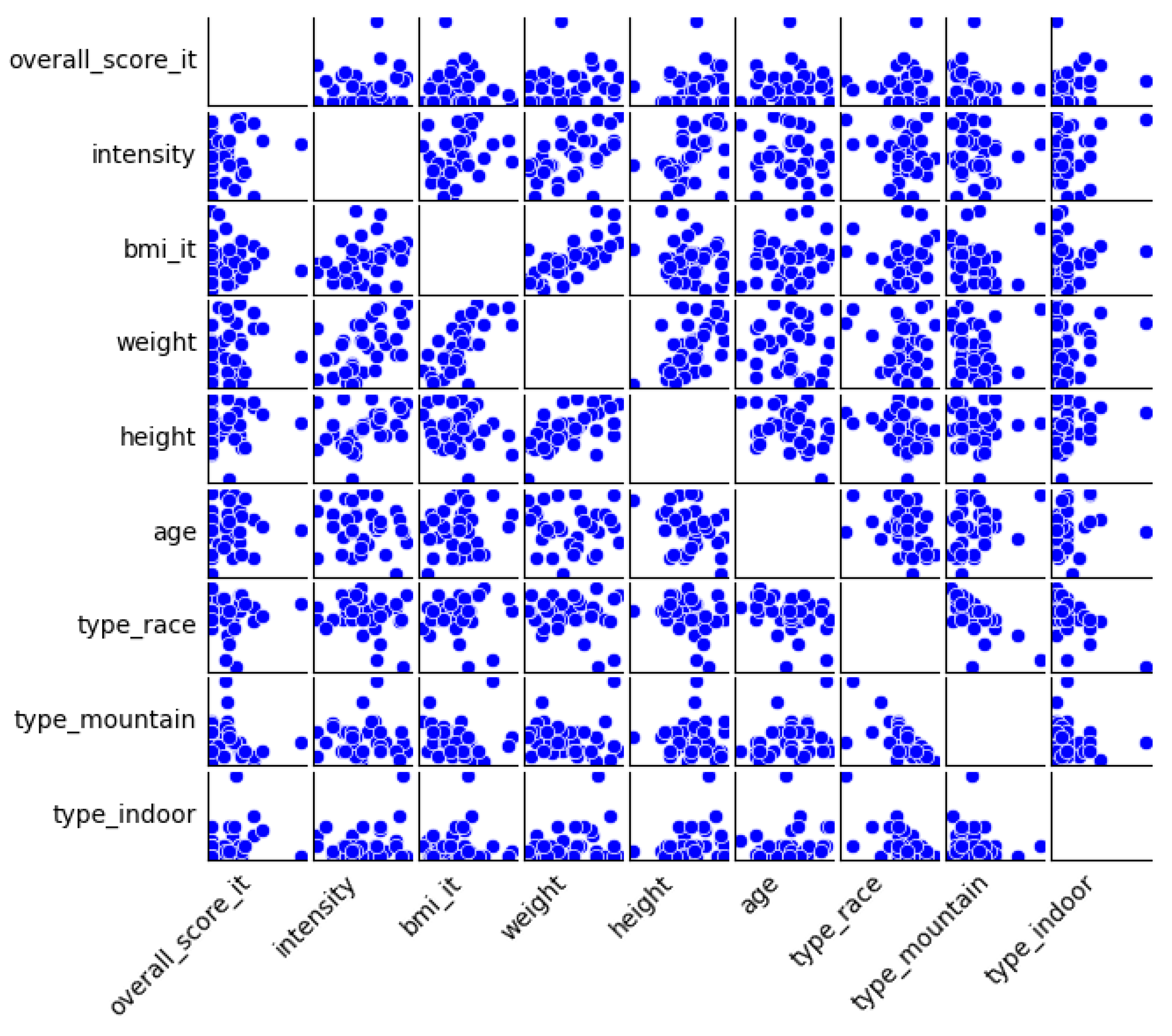
Table 3.
The total number of complaints and share of individuals per group, who reported a particular complaint and injury for each body part. Complaints are ranked by their total number in the sample. Complaints in this table were measured during the baseline test before the intervention started (Source: own illustration/SPSS).
| Baseline test | ||
|---|---|---|
| Body part | Intervention Group | Control Group |
| Neck/cervical spine | 44.4 % (8) | 23.5 % (4) |
| Knee | 33.3 % (6) | 35.3 % (6) |
| Lumbar spine | 22.2 % (4) | 29.4 % (5) |
| Finger | 22.2 % (4) | 17.6 % (3) |
| Wrists | 16.6 % (3) | 23.5 % (4) |
| Upper legs | 16.6 % (3) | 17.6 % (3) |
| Gluteal | 16.6 % (3) | 11.8 % (2) |
| Shoulders | 11.1 % (2) | 17.6 % (3) |
| Hip joint | 16.6 % (3) | 5.9 % (1) |
| Feet/toes | 11.1 % (2) | 11.8 % (2) |
| Other complaints | 5.5 % (1) | 17.6 % (3) |
| Arms | 5.5 % (1) | 5.9 % (1) |
| Total number of complaints | 40 | 37 |
Table 4.
The sum of the scores of the participants for each body part. Scores in this table were measured during the baseline test before the intervention started (Source: own illustration/SPSS).
Table 4.
The sum of the scores of the participants for each body part. Scores in this table were measured during the baseline test before the intervention started (Source: own illustration/SPSS).
| Baseline test | ||
|---|---|---|
| Body part | Intervention Group | Control Group |
| Neck/cervical spine | 45 | 20 |
| Knee | 32 | 33 |
| Lumbar spine | 28 | 23 |
| Gluteal | 19 | 18 |
| Finger | 20 | 16 |
| Wrists | 15 | 20 |
| Upper legs | 16 | 13 |
| Shoulders | 11 | 15 |
| Hip joint | 21 | 3 |
| Feet/toes | 8 | 9 |
| Other complaints | 4 | 13 |
| Arms | 4 | 4 |
| Sum | 223 | 187 |
Table 5.
The table shows the sums of the scores for each body part, measured during the first post-test and second post-test. The numbers in the brackets represent the changes in the scores compared to the previous test (Source: own illustration/SPSS).
Table 5.
The table shows the sums of the scores for each body part, measured during the first post-test and second post-test. The numbers in the brackets represent the changes in the scores compared to the previous test (Source: own illustration/SPSS).
| First Post-Test | Second Post-Test | |||
|---|---|---|---|---|
| Body part | Intervention Group | Control Group | Intervention Group | Control Group |
| Neck/cervical spine | 15 (-30) | 13 (-7) | 15 (0) | 14 (+1) |
| Knee | 22 (-10) | 27 (-6) | 20 (-2) | 25 (-2) |
| Lumbar spine | 23 (-5) | 5 (-18) | 21 (-2) | 6 (+1) |
| Gluteal | 20 (+1) | 12 (-6) | 15 (-5) | 10 (-2) |
| Finger | 11 (-9) | 10 (-6) | 11 (0) | 10 (0) |
| Wrists | 0 (-15) | 15 (-5) | 0 (0) | 13 (-2) |
| Upper legs | 9 (-7) | 5 (-8) | 9 (0) | 5 (0) |
| Sholders | 0 (-11) | 9 (-6) | 0 (0) | 8 (-1) |
| Hip joint | 18 (-3) | 0 (-3) | 17 (-1) | 0 (0) |
| Feet/toes | 0 (-8) | 9 (0) | 0 (0) | 9 (0) |
| Other complaints | 0 (-4) | 0 (-13) | 0 (0) | 0 (0) |
| Arms | 0 (-4) | 4 (0) | 0 (0) | 0 (-4) |
|
Sum / Average change per participant |
118 (-105) -5.83 |
109 (-78) -4,6 |
108 (-10) -0.56 |
100 (-9) -0,53 |
Table 6.
Simple linear regression model 1 estimates the impact of the intervention on the overall score from the baseline test to the first post-test (Source: own illustration/Python).
Table 6.
Simple linear regression model 1 estimates the impact of the intervention on the overall score from the baseline test to the first post-test (Source: own illustration/Python).
| Variable | Coefficient | Std. Error | t-value | p-value | 95% confidence interval |
|---|---|---|---|---|---|
| Intercept | 12.39 | 2.64 | 4.69 | 0.00 | [7.11, 17.67] |
| Time | -5.83 | 3.74 | -1.56 | 0.12 | [-13.3, 1.632] |
| Group (control group) | -1.39 | 3.79 | -0.37 | 0.72 | [-8.96, 6.19] |
| Interaction term | 1.25 | 5.37 | 0.23 | 0.82 | [-9.47, 11.96] |
R2: 0.06 | R2-adjusted: 0.01.
Table 7.
Regression model 2 estimates the impact of the intervention and additional covariates from the baseline test to the first post-test on the overall score (Source: own illustration/Python).
Table 7.
Regression model 2 estimates the impact of the intervention and additional covariates from the baseline test to the first post-test on the overall score (Source: own illustration/Python).
| Variable | Coefficient | Std. Error | t-value | p-value | 95% confidence interval |
|---|---|---|---|---|---|
| Intercept | 10.83 | 16.78 | 0.65 | 0.52 | [-22.71, 44.36] |
| Time | -5.8 | 3.65 | -1.59 | 0.12 | [-13.09, 1.5] |
| Group (control group) | -4.21 | 3.92 | -1.08 | 0.29 | [-12.05, 3.62] |
| Interaction term | 1.23 | 5.23 | 0.24 | 0.82 | [-9.23, 11.69] |
| BMI | -0.26 | 0.68 | -0.38 | 0.71 | [-1.62, 1.12] |
| Age | 0.32 | 0.19 | 1.67 | 0.1 | [-0.07, 0.71] |
| Type mountain bike | -0.22 | 0.09 | -2.39 | 0.02 | [-0.4, -0.04] |
R2: 0.143 | R2-adjusted: 0.061.
Table 8.
Simple linear regression model 3 estimates the impact of the intervention on the overall score from the first post-test to the second post-test (Source: own illustration/Python).
Table 8.
Simple linear regression model 3 estimates the impact of the intervention on the overall score from the first post-test to the second post-test (Source: own illustration/Python).
| Variable | Coefficient | Std. Error | t-value | p-value | 95% confidence interval |
|---|---|---|---|---|---|
| Intercept | 6.56 | 1.82 | 3.61 | 0.00 | [2.93, 10.18] |
| Time | -0.56 | 2.57 | -0.22 | 0.83 | [-5.68, 4.57] |
| Group (control group) | -0.14 | 2.61 | -0.06 | 0.96 | [-5.35, 5.06] |
| Interaction term | 0.03 | 3.69 | 0.01 | 0.99 | [-7.33, 7.38] |
R2: 0.001 | R2-adjusted: -0.044.
Table 9.
Regression model 4 estimates the impact of the intervention and additional covariates from the first post-test to the second post-test on the overall score (Source: own illustration/Python).
Table 9.
Regression model 4 estimates the impact of the intervention and additional covariates from the first post-test to the second post-test on the overall score (Source: own illustration/Python).
| Variable | Coefficient | Std. Error | t-value | p-value | 95% confidence interval |
|---|---|---|---|---|---|
| Intercept | -8.98 | 12.12 | -0.74 | 0.46 | [-33.2, 15.25] |
| Time | -0.4 | 2.51 | -0.16 | 0.88 | [-5.42, 4.63] |
| Group (control group) | -1.46 | 2.71 | -0.54 | 0.59 | [-6.87, 3.95] |
| Interaction term | -0.11 | 3.60 | -0.03 | 0.98 | [-7.30, 7.09] |
| BMI | 0.42 | 0.50 | 0.83 | 0.41 | [-0.58, 1.42] |
| Age | 0.20 | 0.14 | 1.48 | 0.14 | [-0.07, 0.47] |
| Type mountain bike | -0.11 | 0.06 | -1.77 | 0.08 | [-0.24, 0.02] |
R2: 0.092 | R2-adjusted: 0.005.
Table 10.
Simple linear regression model 5 estimates the impact of the intervention on the overall score from the baseline test to the second post-test (Source: own illustration/Python).
Table 10.
Simple linear regression model 5 estimates the impact of the intervention on the overall score from the baseline test to the second post-test (Source: own illustration/Python).
| Variable | Coefficient | Std. Error | t-value | p-value | 95% confidence interval |
|---|---|---|---|---|---|
| Intercept | 12.39 | 2.89 | 4.79 | 0.00 | [7.23, 17.56] |
| Time | -6.39 | 3.66 | -1.75 | 0.085 | [-13.69, 0.91] |
| Group (control group) | -1.39 | 3.71 | -0.37 | 0.71 | [-8.8, 6.02] |
| Interaction term | 1.27 | 5.25 | 0.242 | 0.81 | [-9.20, 11.75] |
R2: 0.07 | R2-adjusted: 0.03.
Table 11.
Regression model 6 estimates the impact of the intervention and additional covariates from the baseline test to the second post-test on the overall score (Source: own illustration/Python).
Table 11.
Regression model 6 estimates the impact of the intervention and additional covariates from the baseline test to the second post-test on the overall score (Source: own illustration/Python).
| Variable | Coefficient | Std. Error | t-value | p-value | 95% confidence interval |
|---|---|---|---|---|---|
| Intercept | 11.53 | 16.04 | 0.72 | 0.48 | [-20.52, 43.58] |
| Time | -6.45 | 3.57 | -1.81 | 0.075 | [-13.58, 0.68] |
| Group (control group) | -4.17 | 3.83 | -0.37 | 0.71 | [-8.8, 6.02] |
| Interaction term | 1.34 | 5.12 | 0.26 | 0.79 | [-8.88, 11.57] |
| BMI | -0.28 | 0.66 | -0.42 | 0.68 | [-1.59, 1.04] |
| Age | 0.32 | 0.19 | 1.66 | 0.1 | [-0.07, 0.7] |
| Type mountain bike | -0.22 | 0.1 | -2.42 | 0.02 | [-0.4, -0.04] |
R2: 0.156 | R2-adjusted: 0.076.
Table 17.
Regression model 13 estimates the impact of the intervention from the baseline test to the second post-test on the perceived training intensity (Source: own illustration/Python).
Table 17.
Regression model 13 estimates the impact of the intervention from the baseline test to the second post-test on the perceived training intensity (Source: own illustration/Python).
| Variable | Coefficient | Std. Error | t-value | p-value | 95% confidence interval |
|---|---|---|---|---|---|
| Intercept | 3.964 | 0.161 | 24.571 | 0.000 | [3.642, 4.287] |
| Time | 2.954 | 0.228 | 12.948 | 0.000 | [2.499, 3.410] |
| Group (control group) | -0.891 | 0.232 | -3.851 | 0.000 | [-1.354, -0.429] |
| Interaction term | 1.350 | 0.327 | 4.124 | 0.000 | [0.697, 2.004 ] |
R2: 0.885 | R2-adjusted: 0.879.
Disclaimer/Publisher’s Note: The statements, opinions and data contained in all publications are solely those of the individual author(s) and contributor(s) and not of MDPI and/or the editor(s). MDPI and/or the editor(s) disclaim responsibility for any injury to people or property resulting from any ideas, methods, instructions or products referred to in the content. |
© 2025 by the authors. Licensee MDPI, Basel, Switzerland. This article is an open access article distributed under the terms and conditions of the Creative Commons Attribution (CC BY) license (http://creativecommons.org/licenses/by/4.0/).
Copyright: This open access article is published under a Creative Commons CC BY 4.0 license, which permit the free download, distribution, and reuse, provided that the author and preprint are cited in any reuse.


