
Submitted:
24 April 2025
Posted:
25 April 2025
You are already at the latest version
Abstract
We consider melting of a one-dimensional domain (x≥0), initially at the melting temperature u=0, through fixing the boundary temperature to a value u(0,t)=U_0 > 0)–the so called Stefan melting problem. The governing transient heat-conduction equation involves a time derivative and the divergence of the temperature gradient. In the general case the order of the time derivative and the gradient can take values in the range (0,1]. In these problems it is known that the advance of the melt front s(t) can be uniquely determined by a specified prefactor multiplying a power of time related to the order of the fractional derivatives in the governing equation. For given fractional orders the value of the prefactor is the unique solution to a transcendental equation formed in terms of special functions. Here, our main purpose is to provide efficient and simple numerical schemes to compute these prefactors. The values of the prefactors are obtained through a dimensionalization that allows the recovery of the solution for the quasi-stationary case when the Stefan number approaches zero. The mathematical analysis of this convergence is given, providing consistency to the numerical results obtained.
Keywords:
fractional Stefan problem
; free boundary
; Caputo derivative
1. Introduction
The Stefan problem of melting is a well known free boundary problem that has been deeply studied in the last century. The scope of this model is very broad, as can be seen in the review article [26] which cites and compiles more than 5000 articles on Stefan problems up to the year 2000.
When we deal with one-dimensional Stefan problems, under certain initial and boundary conditions, the motion of the free boundary (the melt front) behaves as the square of time t[1,16]. In particular, if we address the one-phase Stefan problem with a constant boundary condition, that is, if we consider the problem to find the pair of functions representing the temperature and the advance of the interface, such that
then the free boundary is given in terms of the square root of time,
where is the positive solution to the transcendental equation
We call the prefactor of the free boundary because, clearly, the advance of the interface is totally characterized by this number. The relevance of computing this parameter (which is relatively easy nowadays) was exposed by Solomon in [24] by giving exact data and demonstrating the importance of similarity solutions in semi-infinite domains to approximate exact solutions.
The heat transport governing equation in the Stefan problem above, (1), is the classical diffusion equation. This equation arises as a consequence of inserting the phenomenological Fourier law for heat transfer into the heat continuity equation (first law of thermodynamics). However, the Fourier law is not the only way to model heat transfer. The theory of non-Fourier heat transfer is highly diverse, as can be observed, for instance, in Zhmakin’s book [31] or the work [23]. Such treatments are suitable to model heat transfer in the presence of fractal structures, or amorphous materials like glassy polymers [2] or silica glasses [13]. The focus of this article is a particular class of non-Fourier heat transfer models, namely those that employ fractional calculus to describe anomalous diffusion. More explicitly, we consider here non-Fourier models in presence of fractional integrals or derivatives of Riemann-Liouville or Caputo type. We refer the readers to the works of Metzler and Klafter [17] and Voller [29] which provide an in-depth discussion on the modeling of anomalous diffusion processes using fractional derivatives, as well as the books [9,10,15,18,22] for the theory and applications of fractional diffusion equations.
When the presence of anomalous diffusion is considered in a free boundary problem with an imposed constant temperature at the fix boundary, an interesting feature emerges: the advance of the free boundary is proportional to a power of t that differs from (see e.g. [21] or [28]). That is,
when the process is referred to as superdiffusive and when as subdiffusive.
We are strongly convinced that fractional models can be valuable when emphasizing the evolution of the free boundary. Thus, mirroring classical work on Stefan problems [24], our goal here is to develop algorithms and techniques to compute the prefactor associated with both super- and sub- diffusive one-dimensional, one-phase Stefan melting problems. In carrying out this task we will use the similarity solutions of anomalous Stefan problems that has been previously presented in the literature. In this light, we emphasis that the key component in our work is to arrive at computations that produce explicit numerical values for the prefactors . Beyond their intrinsic value, such results are useful in validating the effectiveness and accuracy of numerical methods for phase-change problems in presence of anomalous diffusion, e.g., [4,7,8,11]. As a verification of our proposed computations we provide a mathematical analysis that shows that when the governing dimensionless group, the Stefan number , our calculations for converge to the known explicit values associated with quasi-stationary anomalous Stefan problems [21,28].
Our paper is laid out as follows. In Section 2, the time fractional and space fractional Stefan problems for a melting process are presented. Section 3 is devoted to the a dimensionless scaling of such problems, focusing on the role of the Stefan number in each case. Section 4 and 5 deal with the space fractional and time fractional cases, respectively, having both the same structure. The selfsimilar solutions for the general and the stationary problems are presented first. Then a method for the computation of the prefactor is presented and finally, an analytical proof of the convergence of the prefactors of the general solutions to the prefactors of the quasi-stationary solution when the Stefan number approaches zero, is given. Finally we present the conclusions and future work in Section 6.
2. Modeling the Space and Time Fractional Stefan Problems in a Melting Process
Suppose that is a cylinder of anomalous phase change material with constant cross-section A and length , where is an isolated extreme. Let be the temperature of the cylinder at position x and time t and let be the heat flux. We assume that, initially, the bar is at its melt temperature and a melting process with a sharp moving interface is initiated by imposing a constant temperature at . This free boundary, representing the moving melt interface, is assumed to be an increasing function in time, i.e,
The total energy in the model is given by the enthalpy
where the thermophysical parameters at the liquid phase are the specific heat c and latent heat ℓ, which is the energy used in the phase change. With this definition we can use the basic thermodynamic principles to recover two balance statements:
The balance of energy in the liquid melt,
where is the material density and the of balance energy at the interface where the phase change occurs,
This is recognized as the classical Rankine–Hugonoit condition, the double brackets representing jumps in the enthalpy and the heat flux respectively and the velocity of the free boundary.
It is well known that equation (1) is obtained after replacing the classical Fourier law in the balance equation (6). This law states that the local heat flux q at a point x is proportional to the gradient of temperature
where we have assumed that the conductivity of the material k is constant. By contrast, here we consider a non-local flux law defined by the relation
This equality states that the flux at every time t and position x is a generalized sum of all the local fluxes at every position between the left extreme of the slab () and the current position, imposing the condition that the local fluxes “closer” to the current position have more weighting than the local fluxes “further” away. Note the constant is defined by
where is a parameter that has been added to preserve the physical dimensions.
At this point let us recall the classical definitions of fractional calculus that will be used in this article.
For every we define the fractional integral of Riemann-Liouville of order by
Now, for we define the fractional derivatives of Riemann-Liouville and Caputo of order , respectively, by
and
a.e. in . The possibility to define these functions at must be analyzed in every case.
With these fractional derivative definitions in hand we can provide non-local definitions of the flux. In particular we note that (9) can be expressed in terms of the Caputo derivative
referred to as the Caputo flux. In this way, replacing (11) in the balance equations (6) and (7) we obtain the governing equations of the space fractional Stefan problems considered in this article
and
Here we have used (5) to compute
Also, we have assumed that the non-local flux at the solid phase is given in terms of the local fluxes between the current position and the right extreme , that is by
which, according to (5), yields that for every . Then
Thus, on defining the region and providing appropriate initial and boundary conditions we obtain the Space Fractional Stefan Problem: Find the pair of functions and with enough regularity such that
We move now to defining a time fractional model, achieved through introducing the concept of memory enthalpy in the balance equations.
where and is a parameter that has been added to preserve dimensional consistency. It is important to stress that expression (15) corresponds to a continuous function that converges pointwise1 to when , and thus it can be interpreted as a regularization of the piecewise function which presents a finite jump at the interface. The idea of considering a regularized enthalpy is a common idea in the literature [3,27,30], the novelty of the approach here is to achieve this through a fractional integral as opposed to the more standard approach of allowing the phase change to occur smoothly over a small temperature region–a mushy zone.
On joining (4), (5) and (15) we have that
Then, by replacing (16) and (8) in the balance equation (6) we obtain the governing equation in the liquid region
or equivalently
For the condition at the interface, we use the continuity of the memory enthalpy to deduce that
Then the classical Stefan condition at the interface (1) is “lost” in the memory enthalpy model and it can be replaced by
Remark 1.
Condition (20) was previously obtained for the memory flux Stefan problem in [14] and later in [21]. It is a natural condition for the memory enthalpy problem, which comes from the continuity of the “memory enthalpy” at the interface.
Following from the above analysis, we can present the Time Fractional Stefan Problem: Find the pair of functions and with enough regularity such that
3. The Dimensionless Problems
In this subsection, we aim to rewrite problems (14) and (21) in a dimensionless form, allowing us to recover the quasi-stationary problems associated with each case in the limit as the dimensionless Stefan number approaches zero. Note that the dimensionless form of the time fractional problem has previously been derived in [19][Prop. 8], the addition of the spacial fractional case is new.
To start our derivations of the dimensionless problem formulations we identify the dimensions of the problem properties in Table 1 and provide a Proposition 1 to determine the dimensions of fractional derivative operators.
Proposition 1.
For every it holds that:
- (1)
- .
- (2)
- .
- (3)
- .
Proof.
We only give the proof of 1, which is a simple compute.
□
Remark 2.
At this point it is important to stress that the classical change of variable for the time, which is generally defined by and , is not used in this article because we are specially interested in obtaining a non-dimensional model that permits to obtain the quasi-stationary case when the dimensionless Stefan number (see Table 1) approaches zero.
The importance given to the quasi-steady-state case lies in the fact that we exactly know the value of the prefactor of the free boundary for any given fractional order .
3.1. The Dimensionless Spacial Fractional Stefan Problem
To simplify, without loss of generality, we rewrite problem (14) with the melt temperature .
First, let us clarify the units of measure of the parameter which was added to give physical dimension consistency. The appropriate dimensions follow directly from the governing equation (22)-(i). By applying Proposition 1 and the dimensions noted in Table 1 to this equation we arrive at the following dimensional balance
which implies that
Change of variables for the Space Fractional case. If we let be a characteristic position we can define the the following dimensionless space and time variables in terms of the quantities in Table 1
In addition, on using as the characteristic temperature, we can construct dimensionless dependent variables for temperature and front position as
Then, by making the substitution in the fractional integral, we have
And
3.2. The Dimensionless Time Fractional Stefan Problem
Let us work now with problem (21) for the case . That is, consider the problem to find the pair of functions and with enough regularity such that
As before, we start by clarifying the role of the parameter . But first, it is important to introduce an equivalent problem to (36) that will be used in this subsection. More precisely, according to [21, Prop. 5], problem (36) is equivalent to the problem to find the pair of functions and such that
Note that we can rewrite equation (37) by using the diffusion coefficient and defining in the following way.
From this equation, using Proposition 1, Table 1, we obtain the dimensional balance
From which it follows that
Remark 3.
Consistent with Remark 2, we consider the non-classical change of variable (25) in order to achieve the quasi-stationary problem when the Stefan number approaches zero.
Change of variables for the Time Fractional case. Let be a characteristic position and consider the change of variables (25). We define as before,
where and are related by (25). Applying the substitution in the following integral, we deduce that
Also,
Then
From the other side,
Substituting (42), (43) and (44) in (38) gives
Note that is an admissible parameter verifying (40). Then by replacing this parameter into (45) and addressing with initial and boundary conditions, the following dimensionless problem associated to the Time Fractional Stefan Problem is obtained: Find the pair of functions and enough regular such that
4. Computing the Prefactor for the Space Fractional Case
4.1. Closed Solutions
Let us start with the quasi-stationary case. This problem is usually attained by making the specific heat . The resulting problem is trivial in (14) or (21) but we focus now in problem (35). Thus, by assuming that the latent heat ℓ and the imposed temperature are finite positive numbers, it is immediately clear from the Stefan number definition in Table 1 that
Then, the limit problem obtained from (35) by making is the Space Fractional quasi-Stationary Problem: Find the pair of functions and with enough regularity such that
Remark 4.
The change of variable performed in (25)-(26) and (41) remains unaffected when considering the limit . Indeed,
is independent of c.
Problem (48) was solved in [28] and its close solution is given by the pair
We now present an exact solution to problem (35), originally introduced in [20], which has been adapted here for the dimensionless case with the Stefan number as the main parameter. To that end, let us introduce the special functions involved
Definition 1.
Let , and l such that . The three-parametric Mittag-Leffler function is defined by
Remark 5.
A particular case is and we recover the classical Mittag-Leffler function for and . Also, a two parametric Mittag–Leffler function is recovered for the case and the special case of our interest is For the role of the three-parametric Mittag-Leffler function we refer the reader to the original works of Kilbas and Siago
We will consider the parameters . For this case we have
and the coefficients verify the next recursive form
We know from [12,Th.1] that the three-parametric Mittag-Leffler functions (50) already defined are entire functions for every .
Define the function by
Now, by mimicking the steps in [20, Section5], it is straightforward that the pair given by
and
where is the unique solution to the equation
is the solution to problem (35).
Remark 6.
Let us highlight that the expression for theprefactor of the free boundarythat we are trying to approximate is given by
The results in the next proposition can be founded in [20, Prop.8 and Section5].
Proposition 2.
The function given in (53) verifies the following properties:
- 1.
- is a non-negative function such that .
- 2.
- The following limits hold:
- 3.
- The function given by is a decreasing function.
4.2. Computing
Using series expansion of in the definition of we can rewrite the equation (56) as
The solution to the last equation (59) can be interpreted as the root of the following function in the left hand side. Thus, a simple method like the bisection method can be applied to find the solution to (59), after making an efficient computation of the 3-parametric Mittag-Leffler functions (in [5], a simple code is presented to see how it has been computed).
4.3. Analysis of the Convergence to the Quasi-Stationary Case
As it was stated in Section 3, the quasi-stationary problem is obtained by making the sensible heat in (35). However taking into account (47) and being the Stefan number the visible parameter in our equations, the convergence to the quasi-stationary case will be analyzed by making . It is also worth noting that the convergence analysis is not affected by the change of variable, according to Remark 4.
In view of the results obtained from the previous algorithm for for a fix (see Table 2), the next theorem is presented.
Theorem 1.
Proof.
For every let the unique positive solution to (56). Equivalently, verifies the equation
where H is the function defined in Proposition 2. Let . If we suppose that , from Proposition 2 item 3 we deduce that . Then, , which is a contradiction. Then the family is decreasing respect on the parameter and being the positiveness of the elements we deduce that Now, making in (56) yields that and from Proposition 2 we have
Now, using (56) again
From (61) and Proposition 2,
Finally, we make in (62) and use (63), (64) and the property of the Gamma function saying that to obtain
□
Corollary 1.
5. Computing the Parameter for the Time Fractional Case
5.1. Close Solutions
Let us start by introducing the special functions involved in the representation of the solution for the time fractional case. For more details we refer the reader to [25]
Definition 2.
For every , the upper incomplete Beta function of parameters is given by
Also, the regularized upper incomplete Beta functions is defined by
Here, is the classical Beta function defined by .
Remark 7.
Note that the former functions are not symmetric respect to the parameters α and β, in contrasts to the classical Beta function which verifies that
Proposition 3.
For all , it holds that
Proof.
Applying Fubini’s theorem, we have that
and the thesis holds by using the Beta function definition and (71). □
We start with the quasi-stationary problem. That is, we consider the limit problem obtained from (46) by making (or equivalently ), which is the Time Fractional Quasi-Stationary Problem: Find the pair of functions and with enough regularity such that
where is the function given by
Problem (74) was already addressed in [21], where the following solution was obtained:
Regarding the non-stationary problem (46), we must refer first to the work of Kubica and Ryszewska [14] where a similarity solution was obtained. However, unlike the solution here, this solution was not presented in a compact form in terms of calculable transcendental functions. To more clearly see this, we present a selfsimilar solution following the lines in [14]. To begin, let us recall the formulation of Problem (46).
Let us define the one variable function in terms of a self-similar variable (which is different than the one considered in [14]).
And let the free boundary be given by
Remark 8.
We have made a simplification in the notation by denoting , in the aim to simplify the reading of the next computes. And the correct notation will be recovered at the end of this section.
We have
From the boundary condition (77) and making the substitution , it holds that
Also
Then u is a solution to the fractional PDE (77) if and only if F is a solution to the fractional ODE
or equivalently
Note that condition (77) implies that . Then, integrating (84) between and 1 yields
Let us work with the integrals in the r.h.s of (85) starting from the second one.
In the first one we apply Fubini and proceed as in (86) to get
By replacing (86) and (87) in (85) we obtain
Now, proceeding as in [14] we define the function
and the operator such that
Then verifies
It is important to recall that we have written the operator L and function G in terms of the incomplete Beta function, but the work and estimations done in Section 5.3 and 5.4 of [14] are valid for these expressions. The recursive argument is also valid, consisting of applying the operator L to both sides of equation (91) and use eq. (91) to recover a new equation for times, yielding that
In [14,Secc.5.2] it was proved that taking the limit when in (92) yields that
And integrating between and 1 and using condition (46) we get an expression for F which is
The uniform convergence of the series in (93) as well as the regularity of function F were analyzed in the mentioned paper. We look now for the parameter a, by using the boundary condition (77). In other words, we look for a positive value a such that
where from (90) and denoting , the operators are given by
for and we define as .
In order to obtain an expression in terms of the powers of the parameter , we redefine the operators as follows. First we define
and then we replace it in (95), multiply both sides by , and we deduce that the prefactor a verifies that
Now, define the function
We know from [14][Secc- 5.2] that the series in (98) is absolutely convergent and thus the function is a well defined continuous function. Moreover, is an increasing and positive function. Thus, the equation
admits a unique positive solution, named and we can recover a asking that
More precisely, recalling the definition of , we state that the prefactor a is given by
5.2. Computing
In this section, we outline the elements needed to compute the prefactor a. i.e. the coefficients . After this computation, the value of a is achieved using the nonlinear equation (99) in a similar way than before (see [5] for details on the computation).
For that purpose, let us focus on the coefficients defined in (97).
Proposition 4.
For every the coefficients defined in (97) verify that
Proof.
We prove first that, for every
In fact, applying (96), Fubini’s Theorem and making the substitution in the penultimate equality, we get
Repeating the former argument times and using (96) we obtain
which completes the proof.
□
We also present the following property needed for next section.
Proposition 5.
For all , it holds that .
Proof.
It immediately follows from the positiveness of
and formula (103). □
5.3. Analysis of the Convergence to the Quasi-Stationary Case
Following a similar approach presented in Section 4.3, and recalling (47), the analysis of convergence will be state by making .
Theorem 2.
Proof.
Let the unique positive solution to .
By Proposition 5, we deduce that , and . Then, from this comment and equality
it holds that .
We can compute now the following limit
□
Corollary 2.
Proof.
First, note that, being for all , it follows that
By induction, we deduce that
Then,
and for the series in the right-hand-side converges absolutely. Hence, using that for all when , we obtain that
and the convergence is proven.
□
6. Conclusions
We have presented selfsimilar solutions for one-dimensional time and space fractional Stefan melting problems; problems directly derived from thermodynamically consistent balance laws. It is well known that, when a constant temperature boundary () is applied and the initial position of the sharp interface is the origin (), these solution exhibit sub- and super- diffusion behaviors respectively, i.e., the melt front advance is determined as the product of a prefactor and time to a power n, different from the diffusion value of . In both the fractional time and space cases, the time exponent is given in terms of known functions of the orders of the space and time derivatives in the problem formulations. The main contribution of the current work has been to, for the first time, make explicit computations for the values of the prefactors. We expect that our analysis will be useful when proposing fractional models for anomalous diffusion. Besides, the exact solutions (prefactor values) computed here will be a strong tool for testing numerical methods for fractional free boundary problems.
Author Contributions
Conceptualization, Mathematical Analysis, Writting, S. Roscani, L. Venturato and V. Voller. ; Conceptualization and Numerical Methods, N. Caruso.
Acknowledgments
S. R., L. V. and N. C. where supported by the projects Proyectos Austral N°006-25CI2001 from Universidad Austral, PIP N° 11220220100532 from CONICET, 80020230300102UR from UNR. S.R. was supported by PICT-I-INVI-00317.
Conflicts of Interest
“The authors declare no conflicts of interest.”
References
- Alexiades, V.; Solomon, A. D. Mathematical Modelling of Melting and Freezing Processes, Hemisphere: Taylor and Francis, Washington, 1993.
- Arya, R. K.; Thapliyal, D.; Sharma, J.; Verros, G. D. Glassy Polymers—Diffusion, Sorption, Ageing and Applications Coatings 2011 11 (9), 1049. 11 (9).
- Bertsch, M.; Klaver, M. The Stefan problem with mushy regions: Differentiability of the interfaces, Ann. Mat. Pura Appl., 1994, 166, 27–61. [Google Scholar] [CrossRef]
- Błasik, M.; Klimek, M. Numerical solution of the one phase 1D fractional Stefan problem using the front fixing method Math Method Appl Sci 2015,38(15), 3214–3228.
- Caruso, N.; Roscani, S.; Venturato, L. carusonahuel/FractionalStefanProblems_Computing_prefactors: Computing prefactors (v1.0.0). Zenodo. [CrossRef]
- Feng, Y. ; Goree, J; Liu, B. Identifying anomalous diffusion and melting in dusty plasmas Phys Rev E 2010, 82. [Google Scholar]
- Garshasbi, M.; Sanaei, F. Studying a time-fractional moving boundary diffusion model of solvent through a glassy polymer: A computational approach. Int J Numer Model 2024, 37(2), e3181. [Google Scholar] [CrossRef]
- Gruber, C. A.; Vogl,C. J.; Miksis,M. J.; Davis,S. H. Anomalous diffusion models in the presence of a moving interface. Interfaces Free Bound 2023, 15(2), 181–202. [Google Scholar] [CrossRef]
- R. Hilfer. Applications of Fractional Calculus in Physics, 2000.
- Jin, B. Fractional differential equations; Springer, Switzerland, 2021.
- Kang, J.; Zhou, F.; Xia, T.; Ye, G. Numerical modeling and experimental validation of anomalous time and space subdiffusion for gas transport in porous coal matrix. Int J Heat Mass Tran 2016, 100, 747–757. [Google Scholar] [CrossRef]
- Kilbas, A.A.; Saigo, M. On Mittag-Leffler type function, fractional calculus operators and solutions of integral equations. Integr Transf Spec F 1996, 4(4), 355–370. [Google Scholar] [CrossRef]
- Kukhtetskiy, S. V.; Fomenko, E. V.; Anshits, A. G. Anomalous Diffusion of Helium and Neon in Low-Density Silica Glass. Membranes 2023, 13(9), 754. [Google Scholar] [CrossRef] [PubMed]
- Kubica, A. and Ryszewska K. A self-similar solution to time-fractional Stefan problem,Math Methods Appl Sci2021, 44(6), 4245–4275.
- D. Kumar and J. Singh. Fractional Calculus in Medical and Health Science. 2020.
- Meirmanov, A. The Stefan problem. Walter de Gruyter, Berlin, 1992.
- Metzler, R.; Klafter, J. The random walk’s guide to anomalous diffusion: a fractional dynamics approach. Phys Rev 2000, 2000 339, 1–77. [Google Scholar] [CrossRef]
- I. Podlubny. Fractional Differential Equations, 1999.
- Roscani, S.; Caruso, N.; Tarzia, D. Explicit solutions to fractional Stefan-like problems for Caputo and Riemann–Liouville derivatives Commun Nonlinear Sci Numer Simul2020,90, 105361. 90.
- Roscani, S.; Tarzia, D.; Venturato, L. The similarity method and explicit solutions for the fractional space one-phase Stefan problems, Fract Calc Appl Anal 2022,25, 995–1021. 25.
- Roscani, S.; Voller, V. On an enthalpy formulation for a sharp-interface memory-flux Stefan problem, Chaos Solitos Fract 2024, 181, ID 114679.
- Samko, S.; Kilbas, A.; Marichev, O. Fractional Integrals and Derivatives–Theory and Applications Gordon and Breach, New York, 1993.
- Schwarzwälder, M. C. , Myers, T. G. and Hennessy, M. G. The one-dimensional Stefan problem with non-Fourier heat conduction. In International Journal of Thermal Sciences,2020, 150.
- Solomon, A. D. An easily computable solution to a two-phase Stefan problem., Solar Energy1979, 23(6), 525–528.
- Srivastava, H. M.; Choi, J. Zeta and q-Zeta Functions and Associated Series and Integrals. Elsevier, London, 2012.
- Tarzia, D. A. A bibliography on moving–free boundary problems for the heat diffusion equation. The Stefan and related problems. MAT–Serie A.
- Ughi, M. A Melting Problem with a Mushy Region: Qualitative Properties, IMA J Appl Math 1984, 33(2), 135–152.
- Voller, V. R. Fractional Stefan problems Int J Heat Mass Transf 2014, 74, 269–277. 74.
- Voller, V. R. Anomalous heat transfer: Examples, fundamentals, and fractional calculus models. In Advances in Heat Transfer; Elsevier 50, 2018; pp. 333–380.
- Voller, V. R.; Cross, M.; Markatos, N. C. An enthalpy method for convection/diffusion phase change Numerical Methods in Thermal Problems1987,24, 271–284. 24.
- Zhmakin, A. I. Non-Fourier Heat Conduction. From Phase-Lag Models to Relativistic and Quantum Transport. Springer, Cham, Switzerland,2023.
| 1 | We refer the readers to Theorem 2.7 in [22] which states that, if , then |
Figure 1.
Space Fractional Stefan Problem. Convergence of (central box) given in (57) to the prefactor of the quasi-stationary case (right column) given in (49).
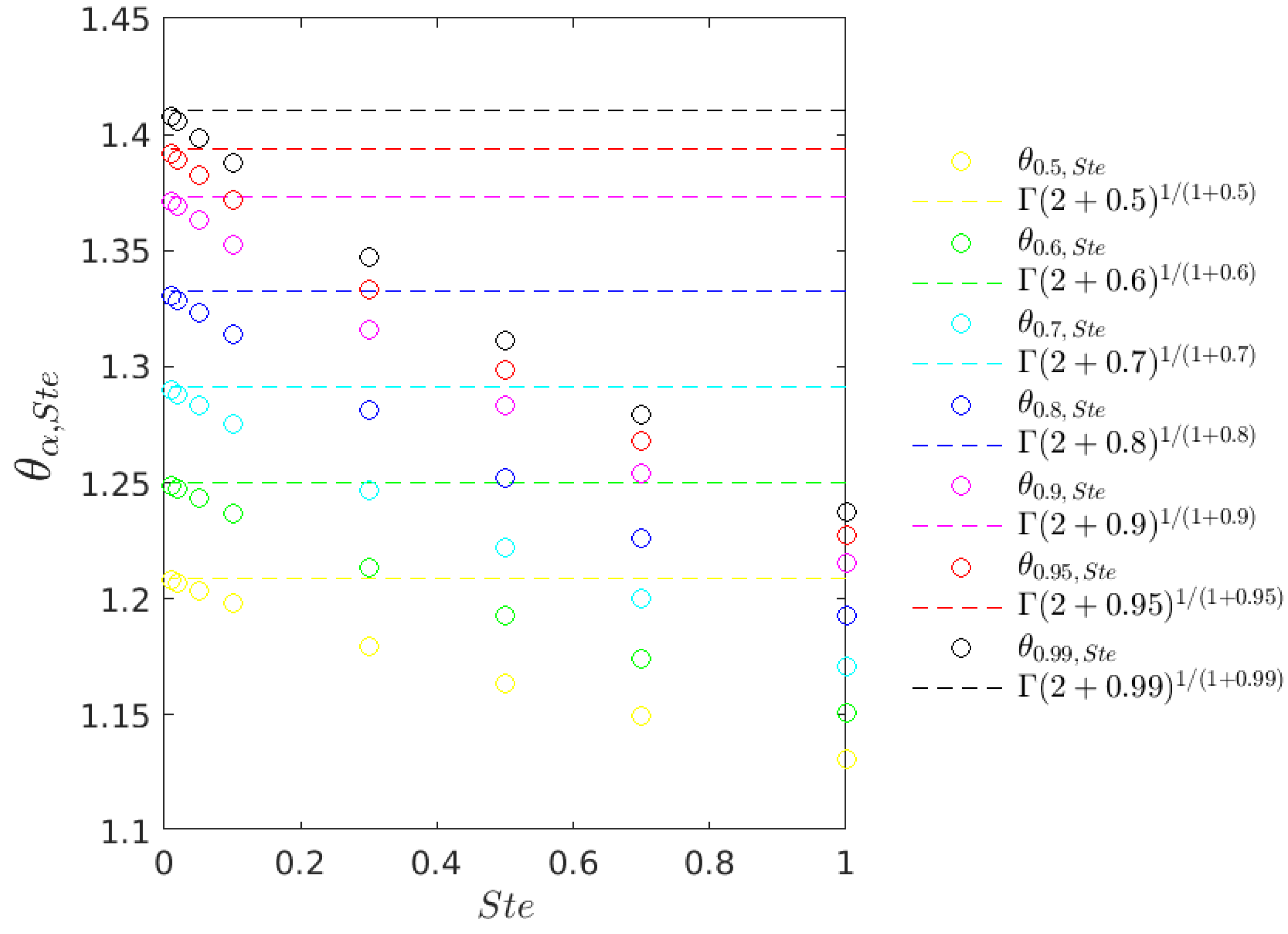
Figure 2.
Time Fractional Stefan Problem. Convergence of to the stationary case
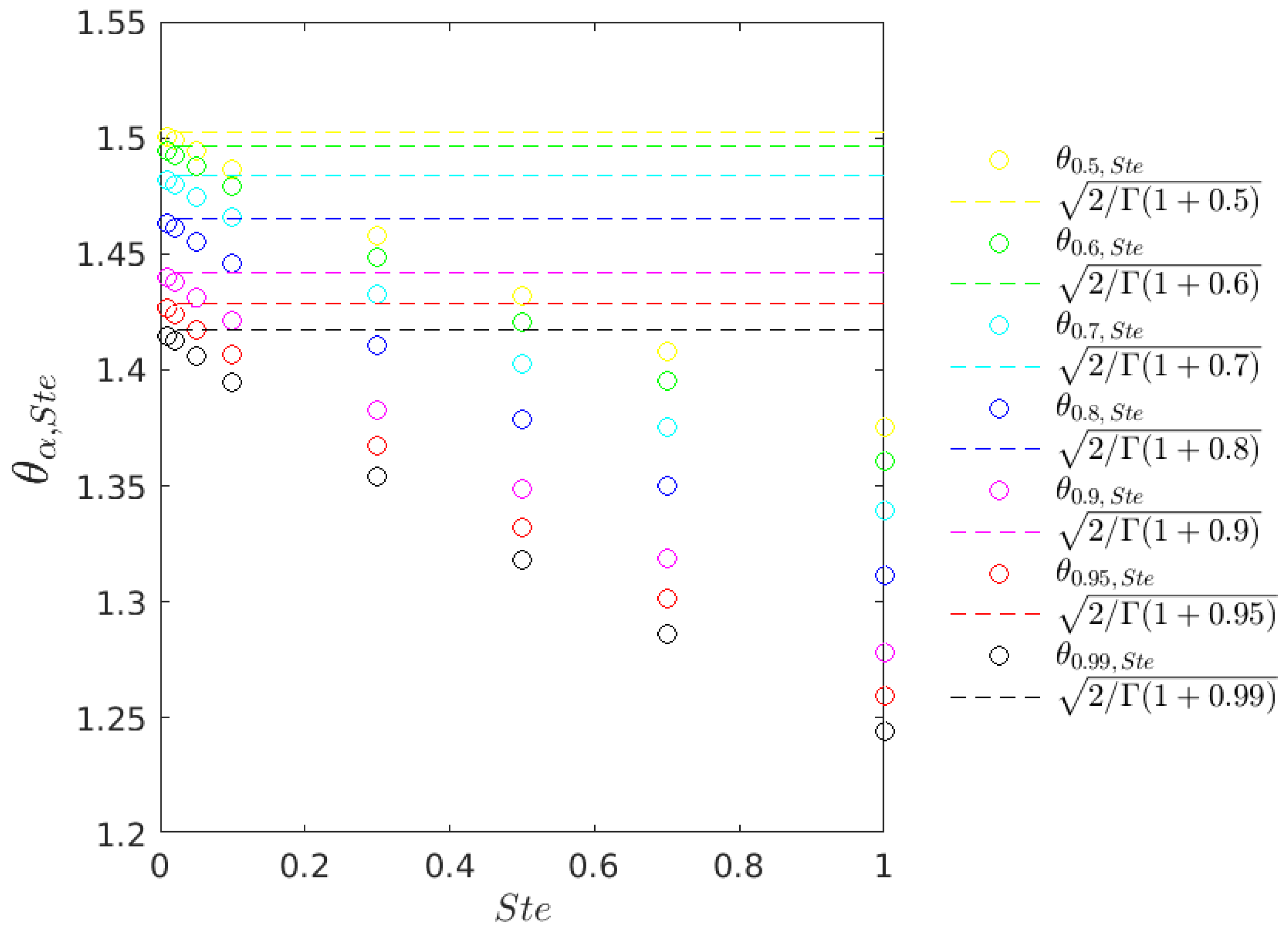

Table 1.
Nomenclature table with property dimensions; [M] mass, [T] time, [L] length, and [K] temperature.
Table 1.
Nomenclature table with property dimensions; [M] mass, [T] time, [L] length, and [K] temperature.
| Symbol | Definition | Dimension |
|---|---|---|
| u | Temperature | [K] |
| x | Spatial position | [L] |
| t | time | [T] |
| k | thermal conductivity | |
| mass density | ||
| c | specific heat | |
| diffusion coefficient | ||
| ℓ | latent heat per unit mass | |
| Stefan number | [-] |
Table 2.
Space Fractional Stefan Problem. Different values of (central box) given in (57) and the prefactor of the stationary case (right column) given in (49).
| [width=3em]Ste | 1.00 | 0.70 | 0.50 | 0.30 | 0.10 | 0.05 | 0.02 | 0.01 | 0 |
|---|---|---|---|---|---|---|---|---|---|
| 0.50 | 1.1311 | 1.1493 | 1.1635 | 1.1797 | 1.1984 | 1.2036 | 1.2068 | 1.2079 | 1.2090 |
| 0.60 | 1.1508 | 1.1744 | 1.1926 | 1.2132 | 1.2370 | 1.2435 | 1.2475 | 1.2489 | 1.2503 |
| 0.70 | 1.1711 | 1.2000 | 1.2221 | 1.2470 | 1.2755 | 1.2833 | 1.2882 | 1.2898 | 1.2915 |
| 0.80 | 1.1926 | 1.2264 | 1.2522 | 1.2811 | 1.3141 | 1.3231 | 1.3287 | 1.3306 | 1.3325 |
| 0.90 | 1.2155 | 1.2539 | 1.2830 | 1.3157 | 1.3528 | 1.3629 | 1.3692 | 1.3713 | 1.3734 |
| 0.95 | 1.2276 | 1.2681 | 1.2987 | 1.3331 | 1.3721 | 1.3828 | 1.3894 | 1.3916 | 1.3938 |
| 0.99 | 1.2376 | 1.2796 | 1.3114 | 1.3471 | 1.3876 | 1.3987 | 1.4055 | 1.4078 | 1.4101 |
Table 3.
Time Fractional Stefan Problem. Different values of (central box) and (right column)
| [width=3em]Ste | 1.00 | 0.70 | 0.50 | 0.30 | 0.10 | 0.05 | 0.02 | 0.01 | 0 |
|---|---|---|---|---|---|---|---|---|---|
| 0.50 | 1.3751 | 1.4077 | 1.4318 | 1.4580 | 1.4867 | 1.4944 | 1.4991 | 1.5007 | 1.5023 |
| 0.60 | 1.3606 | 1.3951 | 1.4206 | 1.4485 | 1.4794 | 1.4876 | 1.4927 | 1.4944 | 1.4961 |
| 0.70 | 1.3391 | 1.3755 | 1.4026 | 1.4324 | 1.4656 | 1.4744 | 1.4799 | 1.4818 | 1.4836 |
| 0.80 | 1.3114 | 1.3498 | 1.3786 | 1.4103 | 1.4459 | 1.4555 | 1.4614 | 1.4634 | 1.4654 |
| 0.90 | 1.2782 | 1.3186 | 1.3490 | 1.3829 | 1.4210 | 1.4313 | 1.4377 | 1.4399 | 1.4421 |
| 0.95 | 1.2598 | 1.3011 | 1.3324 | 1.3673 | 1.4068 | 1.4175 | 1.4242 | 1.4264 | 1.4287 |
| 0.99 | 1.2441 | 1.2863 | 1.3183 | 1.3540 | 1.3946 | 1.4057 | 1.4125 | 1.4149 | 1.4172 |
Disclaimer/Publisher’s Note: The statements, opinions and data contained in all publications are solely those of the individual author(s) and contributor(s) and not of MDPI and/or the editor(s). MDPI and/or the editor(s) disclaim responsibility for any injury to people or property resulting from any ideas, methods, instructions or products referred to in the content. |
© 2025 by the authors. Licensee MDPI, Basel, Switzerland. This article is an open access article distributed under the terms and conditions of the Creative Commons Attribution (CC BY) license (http://creativecommons.org/licenses/by/4.0/).
Copyright: This open access article is published under a Creative Commons CC BY 4.0 license, which permit the free download, distribution, and reuse, provided that the author and preprint are cited in any reuse.


