Submitted:
23 April 2025
Posted:
24 April 2025
You are already at the latest version
Abstract
Confocal scanning images of rocks play a crucial role in petroleum geology and hydrocarbon exploration, as they can reveal the internal microstructure of rocks with high resolution. This capability is of significant importance for enhancing the understanding of hydrocarbon storage, migration capacity, and production prediction. However, traditional two-dimensional images are unable to comprehensively depict the complex internal structures of rocks, which limits the accurate understanding of rock physical properties and geological processes. Therefore, this paper focuses on the three-dimensional (3D) reconstruction of confocal rock images.Firstly, a series of two-dimensional images containing rich microstructural information is obtained through confocal scanning. Subsequently, a preliminary 3D point cloud is constructed using voxelization methods, followed by triangular meshing. The surface reconstruction is achieved using the greedy projection triangulation method, extracting the 3D surface model of the rock. To enhance the realism of the model, texture mapping techniques are employed to project the color information from the original images onto the 3D model.Through comprehensive evaluation of the accuracy, stability, and visualization effects of the reconstructed model, experimental results demonstrate that the proposed method excels in terms of modeling precision, completeness, visual effects, and processing time. The reconstruction accuracy reaches 85%, with a geometric error of 0.05 millimeters, proving its effectiveness and feasibility.
Keywords:
Confocal
; 3D reconstruction
; greedy projection triangulation reconstruction
1. Introduction
With the continuous development of China’s industrial economy, petroleum, as a crucial industrial resource, plays an increasingly vital role in production [1]. In petroleum geological exploration and development, the parameter analysis and quantitative calculation of reservoir pore structures are of paramount importance for studying the physical properties of rocks, fluid migration patterns, and enhancing the efficiency of hydrocarbon reservoir development [2]. In recent years, methods focusing on the analysis of grain size and pore characteristics based on rock images have been widely applied in the geological field. Through precise analysis of pore characteristics and grain morphology between rock particles, a deeper understanding of the rock properties, reservoir parameters, and fluid characteristics of underground reservoirs can be achieved, thereby effectively improving the waterflood development efficiency of oilfields and significantly increasing oil recovery rates [3]. As the key medium for hydrocarbon storage and migration, the internal pore structure of rocks is complex and intricate, resembling a labyrinth, which directly determines the storage capacity and flow efficiency of hydrocarbons. Therefore, in-depth exploration of the microstructural characteristics of rocks, especially grain size and pore features, has become a core approach to revealing rock attributes and estimating reservoir performance. This not only aids in optimizing hydrocarbon field development strategies but also provides essential theoretical and technical support for the efficient exploitation of hydrocarbon resources, holding significant scientific and practical value.
Currently, methods for three-dimensional (3D) reconstruction of rocks can be broadly divided into two categories: one is 3D digital rock reconstruction based on physical experiments, and the other is 3D digital rock reconstruction based on numerical methods. The physical experiment-based 3D digital rock reconstruction method involves directly acquiring the 3D structural data of rock cores using high-precision instruments [4]. Physical experiment methods include 2D thin-section stacking imaging [5], X-ray computed tomography (CT) scanning [6], and focused ion beam scanning [7]. The core principle relies on high-precision instruments (such as high-power optical microscopes, scanning electron microscopes, or CT imaging devices) to obtain 2D slice images of rocks, followed by 3D reconstruction based on depth information recorded during the scanning process, thereby generating a complete 3D digital rock model. However, such methods can only achieve single observations of the 2D surface of samples. Focused ion beam technology may introduce damage due to changes in the physical morphology of the sample surface during grinding, thereby affecting observation accuracy. Nanoscale CT scanning technology faces the contradiction between resolution and image size, making it difficult to simultaneously achieve high resolution and large-scale imaging, necessitating a trade-off between imaging volume and resolution. Additionally, acquiring 3D pore structure images through physical experiment methods not only requires high-end equipment but is also costly, limiting its widespread application in industrial settings.
The numerical reconstruction-based 3D digital rock reconstruction first obtains actual 3D digital rock data as training samples, then maps the information in the images to the distribution characteristics of rock images in the training samples through mathematical modeling, and finally converts the 2D information into 3D information based on the mapping to reconstruct the 3D digital rock [8]. Currently, common numerical reconstruction methods include Gaussian field method [9,10], simulated annealing method [11], multiple-point geostatistics [12,13], and Markov chain Monte Carlo method [14]. However, the Gaussian field method cannot address the issue of poor connectivity in reconstructed digital rocks; the simulated annealing method is susceptible to modeling constraints, and as the number of constraints increases, the reconstruction process slows down, leading to chaotic rock pore structures [15,16]; multiple-point geostatistics assumes that rock samples have similar structural characteristics in different directions, making it less effective for samples with strong anisotropy, and requires hard data constraints in advance [17]; the Markov chain Monte Carlo method is less suitable for samples with strong heterogeneity [18].
With the development of deep learning, Mosser et al. [19] introduced deep convolutional generative adversarial networks (DC-GAN) into 3D digital rock reconstruction, leveraging 3D convolution to learn the 3D distribution of data and achieving good reconstruction results on the Berea sandstone dataset. However, 3D convolution operations in such methods demand significant computational resources, and the models face issues of instability and convergence difficulties during training. Additionally, DC-GAN requires large amounts of data for training, and the high cost of obtaining rock thin-section data limits the practical application and promotion of this method.
In summary, while physical experiment-based 3D digital rock reconstruction methods offer high precision, they are expensive and complex. In contrast, 2D slice-based 3D digital rock random reconstruction methods are cost-effective and easy to implement but suffer from lower precision and coarser reconstruction results, leaving room for improvement. Compared to traditional random reconstruction methods, generative adversarial network-based 3D digital rock reconstruction shows improved results but still faces challenges such as unstable model training and convergence difficulties. Moreover, existing methods fall short in handling rocks with complex pore structures and strong heterogeneity, resulting in poor pore connectivity.
Therefore, to address these issues, this paper proposes a 3D rock reconstruction technique based on confocal scanning images. Confocal imaging technology can provide high-resolution image data, accurately capturing the microstructural details of rocks, particularly suitable for studying complex pore structures. Additionally, this technology resolves the issue of discontinuous imaging in traditional methods through sequential slice stacking, enabling more complete 3D structural reconstruction. Furthermore, confocal imaging technology offers higher computational efficiency and precision in 3D reconstruction, accurately reflecting pore connectivity and microstructural features, providing a reliable foundation for rock physical property simulation and reservoir parameter analysis. This method involves collecting rock samples and acquiring images under a confocal microscope. The original images are preprocessed, and techniques such as point cloud generation and greedy projection triangulation are used to construct and post-process the 3D model. Performance is enhanced through improved registration, optimized scanning, and denoising algorithms. Finally, the method is tested for accuracy, stability, and visualization effects, providing technical and theoretical support for the study of rock microstructures in fields such as geological exploration.
2. Preparation Three-Dimensional Reconstruction Process
This study collected a series of confocal images that provide high-resolution views of rock surfaces. The three-dimensional (3D) reconstruction process is illustrated in Figure 1. After acquiring the raw image data, the preprocessing stage is initiated, which enhances image quality and lays a solid foundation for subsequent 3D reconstruction. Firstly, the color images are converted into grayscale images, which simplifies the processing of image data while preserving essential texture information of the rock surfaces. Next, histogram equalization is applied to optimize image contrast, making different regions of the rock surface more distinguishable. To further improve the visual quality of the images, adaptive histogram equalization is employed. This technique adjusts enhancement parameters based on the local characteristics of the image, thereby enhancing contrast while avoiding distortion caused by over-enhancement. Finally, mean filtering is implemented to eliminate noise in the images. This filtering method reduces salt-and-pepper noise by calculating the average value of each pixel and its neighboring region and replacing the original pixel value with this average. Using the processed images, a 3D point cloud is generated. With the point cloud data obtained, the greedy projection triangulation algorithm is applied to process the data. This algorithm involves mapping the point cloud onto a two-dimensional plane and performing triangulation on this basis, effectively transforming discrete points into a continuous 3D surface.
3. Acquisition and Preprocessing of Confocal Scanning Rock Images
3.1. Acquisition of Confocal Scanningrock Images
As shown in Figure 2, the Leica TCS SP5 II laser scanning confocal microscope was used in this study to acquire rock images. This equipment consists of several key components, including the light source, stage, optical microscope, computer, and the entire optical system. Below are the detailed specifications of the microscope:
1.Light Source:
The microscope is equipped with four independent excitation channels, covering a spectral range from 400 nm to 800 nm. The specific laser wavelengths are listed in Table 1. In this experiment, the laser wavelength was set to 488 nm.
2.Objective Lens:
The confocal microscope is equipped with three objective lenses with different parameters, as detailed in Table 2. The selection of the objective lens is determined based on the specific requirements of the sample.
3.Scanning Parameters:
The frequency options for image scanning include 100Hz, 200Hz, and 400Hz, while the image resolution offers several options such as 512 × 512, 1024 × 1024, 2048 × 2048, etc.
This study utilizes confocal microscopy to capture transmission, light, and heavy images of existing samples, aiming to reveal the internal microstructure and compositional distribution of the samples. As shown in Figure 3, Figure 4 and Figure 5, the images are divided into three types: transmission images, light images, and heavy images.
Transmission images are formed by transmitted light, which can display the overall structure and mineral distribution of the rock samples. For thin-section samples, transmission images can clearly show the transparency, color, and texture characteristics of minerals, aiding in the identification of mineral types and their spatial distribution. Light images are formed by reflected or scattered light, typically using shorter wavelengths for imaging. These images can highlight the surface morphology, mineral boundaries, and micro-cracks of the rock samples. Heavy images are formed by fluorescence or nonlinear optical effects, usually using longer wavelengths for imaging. For rock samples, heavy images can display the fluorescence characteristics of specific minerals or deep structural information.
In summary, for rock samples, transmission images, light images, and heavy images provide different information from the perspectives of overall structure, surface morphology, and deep features, respectively. Transmission images are suitable for mineral identification and overall structural analysis, light images are suitable for surface feature and microstructure studies, and heavy images can be used for fluorescent mineral identification and deep structural analysis. The combined use of these images can provide comprehensive microscopic information support for this study.
3.2. Contrast Enhancement and Dataset Preparation
Confocal images are often affected by laser scattering, detector noise, and sample fluorescence background during acquisition, leading to reduced image quality, diminished feature contrast, and potential geometric distortions. These factors not only compromise the clarity and accuracy of the images but also increase the difficulty of subsequent analysis. Therefore, preprocessing becomes a crucial step to improve image quality, enhance feature contrast, reduce noise interference, correct geometric distortions, and adapt to subsequent analysis algorithms. Through preprocessing techniques such as denoising, contrast enhancement, and geometric correction, images can be made clearer and features more prominent, thereby providing a more reliable data foundation for subsequent quantitative analysis and feature extraction, ensuring the accuracy and reliability of the research results.
3.2.1. Histogram Equalization
This study employs the histogram equalization algorithm [20] to enhance the contrast of confocal images. The histogram equalization algorithm can increase the contrast between pores and the background in confocal images, enabling better differentiation between pore and background regions. Equalization is achieved by first calculating the cumulative gray histogram based on the gray histogram, and then establishing a mapping relationship between the input image and the output image based on the relationship between the gray histogram and the cumulative gray histogram. The mapping relationship is expressed by Equation (1).
In the equation, and represent the height and width of the image, represents the output pixel, and represents the number of pixels with a gray value of k in the image’s gray histogram. The operational steps are as follows:
- (1)
- Calculate the gray histogram.
- (2)
- Compute the cumulative gray histogram.
- (3)
- Derive the mapping relationship based on steps (1) and (2), and finally output the gray pixel values.
3.2.2. Dataset Creation
A rock cylinder with a height of 10 cm and a diameter of 2.5 cm was scanned to produce 397 slices. After histogram equalization processing, a total of 397 contrast-enhanced rock images were obtained. Each rock image has a resolution of 753×753 pixels, including 99 heavy images, 99 light images, and 99 transmission images. These images were sequentially numbered from 0 to 396.
4. Point Cloud Generation and Triangular Mesh Construction
4.1. Rock Point Cloud Generation
Point cloud generation is the process of transforming 2D image data acquired through confocal microscopy into a 3D discrete point set. During confocal scanning of rock samples, 2D images at different depth levels capture the structural information of the rock. By analyzing these images, the pixel positions of target structures (e.g., mineral grain boundaries, pore contours) are combined with the scanning parameters of the confocal microscope (e.g., scanning step size, coordinate system settings). Using spatial coordinate mapping algorithms, the 2D pixel coordinates are converted into 3D spatial coordinates.
The 3D point cloud data structure is a digital model used to represent and capture objects or scenes in 3D space. This data structure consists of numerous discrete points distributed in a 3D Cartesian coordinate system. Each point explicitly records its precise spatial position, determined by the values of the x, y, and z axes. Additionally, these points may store auxiliary information, such as color data or reflection intensity values, providing a richer and more complete description of the 3D object or scene.
4.2. Weight Rule Definition and Triangular Mesh Construction
In the 3D reconstruction process, holes often appear in the generated mesh models due to insufficient sampling, data loss, or limitations of the reconstruction algorithms. These holes can negatively impact subsequent model analysis. Therefore, existing hole-filling techniques are applied to further stitch and repair the generated 3D pore models. Two critical steps in this process are defining appropriate weight rules and performing triangular mesh construction. Weight rules help determine the positions of newly generated vertices, while triangular mesh construction creates new faces to close the holes.
4.2.1. Weight Rule Definition
Weight rules aim to assign a weight to each vertex on the hole boundary. These weights are used to calculate the positions of new vertices added to fill the hole. Weights can be based on various factors, such as geometric features of the vertices (e.g., curvature, normal vectors), the length of boundary edges, and the area of adjacent faces. In the hole-filling process of 3D models, the definition of weight rules is crucial for determining the positions of newly generated vertices. These rules are typically set based on the geometric and topological characteristics of the hole boundary points, ensuring that the new vertices smoothly and naturally close the hole while preserving the overall geometric properties of the model. This study adopts geometric feature-based weight rules, which rely on vertex characteristics such as curvature, normal vectors, and edge length to reflect the influence of each vertex on the hole-filling shape.
The curvature weight formula is shown in Equation (2), where is the curvature weight of the vertex , is the discrete Gaussian or mean curvature of the vertex, and is the weight factor.
The normal vector difference weight formula is shown in Equation (3), where is the weight of vertex based on the difference of normal vectors, is the unit normal vector of vertex, is the average value of the normal vectors of the edge points of the hole, and rn is the weight factor.
The distance weight formula is shown in Equation (4), which considers the distance from the vertex to the hole center or centroid, adjusting the influence of the vertex based on its position.
Among them, is the distance weight of the vertex , is the centroid coordinate of the hole, and is the weighting factor.
The boundary edge length weight formula is shown in Equation (5), which emphasizes the influence of vertices adjacent to longer boundary edges on the hole shape.
This study comprehensively considers the above weight rules to determine the final weight of each vertex, as shown in Equation (6), balancing the impact of various geometric features on hole filling.Here, represents the set of boundary edges adjacent to the vertex , and denotes the comprehensive weight of the vertex .
In this way, the generation and positioning of new vertices during the hole-filling process can be more precisely controlled, thereby achieving better repair results and improved mesh quality.
4.2.2. Triangulation
In the process of 3D reconstruction, mesh models often exhibit holes due to insufficient sampling, data loss, or limitations in reconstruction algorithms, which can adversely affect subsequent model analysis. Therefore, existing hole-filling techniques are applied to further repair and suture the porous 3D model. During the hole-repairing process, two critical steps are defining appropriate weighting rules and performing triangulation. Weighting rules help determine the positions of newly generated vertices, while triangulation involves creating new triangular facets based on these vertices to close the holes.
The objective of triangulation is to utilize the vertices along the hole boundary and potential newly generated vertices to construct triangular facets that seal the hole. This step requires careful consideration of facet quality to avoid distorted or excessively elongated triangles. Delaunay triangulation maximizes the minimum angle of triangles by satisfying the Delaunay condition: the circumcircle of any triangle contains no other points in its interior. This approach aims to maximize the minimum angle, thereby preventing narrow triangles and yielding high-quality meshes.
The triangulation procedure is detailed as follows:
New Vertex Generation: Compute the positions of new vertices based on weighting rules and the geometric characteristics of the hole.
Vertex Aggregation: Combine the original vertices along the hole boundary with the newly generated vertices into a unified vertex set.
Delaunay Triangulation: Apply Delaunay triangulation to the vertex set to generate new triangular facets. Verify the Delaunay condition by ensuring that no points lie within the circumcircle of any triangle. If a triangle violates this condition (i.e., its circumcircle contains other points), adjust the connections to enforce compliance.
Facet Filtering: Select facets generated by Delaunay triangulation that are entirely confined within the hole region for repair. As illustrated in Figure 9, the resulting triangulation guarantees that no points reside within the circumcircle of any triangle, and this configuration achieves the maximum minimum angle among all possible triangulations.
4.3. Mesh Subdivision and Optimization
In the process of hole-filling for 3D models, mesh subdivision and optimization are two critical subsequent steps that enhance the mesh quality of the repaired regions and the overall geometric details of the model. These steps ensure that the repaired model is not only visually smooth and natural but also geometrically accurate.
4.3.1. Mesh Subdivision
Mesh subdivision is a technique used to increase mesh density and improve mesh distribution. It achieves this by adding more vertices and facets to the existing mesh. Commonly used subdivision methods include Loop subdivision and Catmull-Clark subdivision. Loop subdivision is particularly suitable for triangular meshes, where each subdivision divides every triangle into four new triangles, as illustrated in Figure 10.
In this process, new vertices are added at the midpoint of each edge, and the positions of the original vertices are adjusted. Catmull-Clark subdivision, on the other hand, is suitable for quadrilateral meshes, where each subdivision divides every quadrilateral into four new quadrilaterals. Similar to Loop subdivision, this process also involves adding new vertices at the midpoints of edges and the centers of faces. Since the mesh model reconstructed using MC (Marching Cubes) is a triangular mesh, this paper employs Loop subdivision for mesh refinement. The Loop subdivision algorithm consists of two main steps: adding new vertices (midpoints of edges) and adjusting the positions of the original vertices.
Adding New Vertices:For each edge, the average of the coordinates of its two endpoints is calculated to generate a new vertex (i.e., the midpoint of the edge). For each triangle, this results in the creation of three new vertices.
Adjusting the Positions of Original Vertices:The new position of each original vertex is determined by a weighted average of its own position and the positions of its neighboring vertices. The weights for the vertices are calculated as shown in Equation (7).
Here, n represents the degree of the vertex (i.e., the number of edges connected to the vertex), and denotes the weight assigned to the neighboring vertices when calculating the new position of the vertex.
Finally, new triangular facets are generated using the original vertices and the newly added vertices.
4.3.2. Mesh Optimization
Mesh optimization aims to improve the quality of the mesh by adjusting vertex positions, including reducing distorted triangles, increasing the size of the minimum angle, and more. Common mesh optimization methods include Laplacian smoothing and various energy minimization-based approaches. As shown in Table 3, a comparison is made between these two mesh optimization methods in terms of implementation complexity, computational cost, applicability, model feature preservation, and detail preservation.
From the comparative analysis, it is evident that for the pore reconstruction of confocal scanning rock images, the pore features are complex and intricate. To establish a more realistic rock pore model, this paper adopts energy minimization-based optimization for mesh refinement.
Energy minimization-based optimization is an advanced mesh processing technique that improves mesh quality by minimizing an energy function defined on the mesh. This method can smooth the mesh while preserving important features and details of the model, making it suitable for scenarios requiring highly precise control over mesh quality. The energy function typically incorporates multiple geometric and topological constraints, reflecting the ideal state of the mesh. The optimization process involves defining one or more energy terms, each targeting a specific characteristic of the mesh.
Area Uniformity: Aims to make the areas of all triangles in the mesh as similar as possible, reducing excessively large or small triangles.
Edge Length Uniformity: Seeks to make the lengths of all edges in the mesh as consistent as possible, avoiding elongated triangles.
Angle Optimization: Targets maximizing the minimum angle in the mesh to improve the shape quality of triangles.
Shape Preservation: Minimizes shape changes between the original and optimized meshes, particularly at feature edges and sharp regions.
The energy function E is typically expressed as a weighted sum of the above energy terms:
where shaperepresent the energy terms for area uniformity, edge length uniformity, angle optimization, and shape preservation, respectively. The weights balance the influence of each term.
Optimization Process
1.Initialization: Start with the original mesh and compute the current values of its energy terms.
2.Iterative Optimization: Use mathematical optimization techniques to adjust the positions of mesh vertices, minimizing the energy function E.
3.Termination Condition: Stop the optimization process when the change in the energy function falls below a predefined threshold or when the number of iterations reaches a preset limit.
4.4. Greedy Projection Triangulation Reconstruction Algorithm
The greedy projection triangulation algorithm [21] employs Delaunay triangulation to construct a complete target model. Compared to the Poisson reconstruction algorithm, which can generate a target model but often lacks detailed features due to excessive smoothing and may introduce unnecessary redundant surfaces, the greedy projection triangulation algorithm offers a more balanced approach. Additionally, while the Marching Cubes reconstruction algorithm may miss fine details and generate excessive lines and faces, leading to redundancy and potential holes that degrade reconstruction quality, the greedy projection triangulation algorithm addresses these limitations. Therefore, this paper adopts the greedy projection triangulation strategy and provides a detailed explanation of the algorithm in the following sections.
The greedy projection triangulation algorithm is advantageous due to its simplicity and efficiency, enabling rapid generation of an approximate 3D model from point cloud data. However, the method may not always produce optimal triangulation results because it seeks only local optima at each step, potentially overlooking global geometric properties. Moreover, in certain scenarios, such as sparse or noisy point clouds, the algorithm may generate low-quality triangles. To enhance robustness and reconstruction quality, researchers often integrate additional techniques, such as local feature analysis, point cloud simplification, and advanced triangulation strategies. These improvements enable the greedy projection triangulation algorithm to provide effective 3D reconstruction solutions across various applications.
In the k-d tree-based nearest neighbor search algorithm, for any point q in the input point cloud dataset, the algorithm efficiently identifies its k nearest neighbors using the k-d tree structure, thereby defining a local neighborhood. Based on the search results, the point cloud data is categorized into different types, such as boundary points, free points, completed points, and edge points. Subsequently, a projection plane is constructed using point q and its k nearest neighbors, and the neighboring points are mapped onto this 2D plane.
For any point q in the input point cloud dataset and its neighboring points, there exists a mapping relationship from 3D space to a 2D tangent plane. Specifically, each neighboring point can be uniquely projected onto the tangent plane passing through point q, forming a one-to-one mapping. Using the normal estimation method in the greedy projection triangulation algorithm, the approximate normal vector of each point can be calculated, and the tangent plane can be determined via the plane equation. Assuming the normal vector of a point is m=(A,B,C) and point N(x,y,z) lies on the tangent plane of , the tangent plane can be expressed as Equation (9):
By applying a projection matrix, the 3D point cloud data can be mapped onto a 2D slice plane. Through translation and rotation operations, the projection of the point cloud data on the 2D slice plane can be obtained. The projection matrix is given by Equation (10):
where:
is the translation matrix:
is the rotation matrix around the x-axis by angle α:
is the rotation matrix around the y-axis by angle θ:
Using these formulas, the projection of any point onto its tangent plane can be calculated as shown in Equation (11):
When applying the greedy projection triangulation algorithm to triangulate planar point cloud data, the algorithm selects locally optimal points as expansion seeds, maps the point cloud step-by-step into 3D space based on projection relationships, and iterates until surface reconstruction is complete. The specific steps are as follows:
- Randomly select a point from the point cloud data as the initial seed point.
- Use the k-d tree to perform a nearest neighbor search, connecting the seed point to its nearest neighbors to form an initial edge.
- Calculate the point closest to this edge and construct the first triangle.
- Continue finding the point closest to any edge of the existing triangles and generate new triangles iteratively.
- Repeat the above steps until all points are incorporated, forming a complete topological structure. The algorithm terminates at this stage,as illustrated in Figure 11.
This diagram illustrates the distribution of data points in the feature space, revealing clustering patterns, potential groupings, and outliers. In the k-nearest neighbor graph, the contribution of different features to data point classification or clustering can be evaluated. Features that better separate data points exhibit clearer distinctions in the graph. The diagram also shows local density, with higher-density regions indicating concentrated data points and lower-density regions indicating dispersion. For high-dimensional datasets, the local projection diagram of k-nearest neighbors visualizes the local structure of the data in a lower-dimensional space, aiding in understanding intrinsic relationships within the data.
4.5. 3D Reconstruction Results
Multiple tests were conducted based on the greedy projection triangulation reconstruction algorithm, ultimately achieving 3D reconstruction. Its core concept involves projecting point cloud data onto a 2D plane, performing triangulation on this plane to generate triangular facets, and subsequently constructing a 3D model.
The algorithm accepts a point cloud dataset as input, where each point contains its 3D spatial coordinates. Normals are estimated for each point in the cloud to determine the optimal projection direction. A k-d tree or other spatial indexing structure accelerates the search for nearest neighbors in the point cloud. For each point, neighboring points within its local neighborhood are projected onto a 2D plane based on its normal direction. A triangulation process is then applied to the projected points to form triangular facets. The reconstruction results are illustrated in Figure 13 and Figure 14.
Post-reconstruction, the model can be enhanced with texture mapping, where real-world image details are applied to the 3D model. This significantly improves visual realism and enables more accurate simulation of light-surface interactions during rendering, yielding higher-quality visualization results.
Texture mapping allows the use of lower-resolution geometric models while enhancing visual fidelity through high-resolution textures. This approach reduces computational load and storage requirements without compromising visual quality.
The algorithm demonstrates robust performance in reconstructing complex geometries while maintaining computational efficiency, making it suitable for applications requiring rapid and accurate 3D modeling from point cloud data.
4.6. Experiment and Analysis
4.6.1. Evaluation Metrics
To comprehensively evaluate the 3D reconstruction results of confocal scanning rock images, we employ four metrics: Reconstruction Accuracy (RA), Model Completeness (MC), Processing Time (PT), and Geometric Error (GE). Reconstruction Accuracy quantifies the similarity between the generated 3D model and the actual object. Model Completeness assesses whether the reconstructed 3D model fully captures the structural integrity of the original object. Processing Time measures the total computational duration from image acquisition to the generation of the 3D model. Geometric Error calculates the spatial deviation between the reconstructed model and the ground-truth geometry. These metrics collectively provide a multi-dimensional evaluation framework to rigorously analyze the quality and accuracy of the reconstructed models.
The mathematical formulations of these metrics are defined in Equations (12), (13), (14), and (15):
4.6.2. Experimental Results and Analysis
As shown in Table 4, in the three-dimensional modeling experiments based on confocal images for shale samples, the average reconstruction accuracy was found to be approximately 82% after extensive comparative analysis of a large amount of data. In regions of the shale sample where pores are relatively large and regularly distributed, the reconstruction accuracy could reach around 85%. This is attributed to the accurate coordinate transformation during point cloud generation, which relies on the pixel position information and scanning parameters of the confocal images. Additionally, the triangulation meshing operation could closely conform to the actual structure in these relatively simple areas.
However, in areas where tiny pores and complex laminations intersect in the shale, the reconstruction accuracy significantly decreased to as low as 78%. This is mainly because the structure in these regions is extremely complex, and their features are not clearly and distinctly represented in the confocal images. This poses significant challenges to the subsequent feature extraction and model construction, resulting in a relatively large deviation between the model and the actual structure.
Regarding model completeness, detailed assessment and statistics revealed an average completeness of about 75%. In regions of the shale sample where mineral grains are relatively concentrated and pore connectivity is good, the model completeness could exceed 80%, allowing for a clearer representation of the local rock structure. However, overall, due to the complex lamination structure of shale, the presence of numerous tiny pores and fractures, and frequent changes in mineral composition in some areas, information on these intricate structural features is lost during the image acquisition process. Subsequently, due to limitations of existing technology and algorithms, it is difficult to fully restore the lost information, resulting in the failure to adequately represent many small pore branches and fracture ends in the final model, which severely affects model completeness.
In terms of processing time, thanks to efficient algorithm optimization and powerful computational support, the average processing time for this experiment was reduced to three minutes. During the image preprocessing stage, advanced fast denoising and adaptive contrast enhancement algorithms were employed, taking only about 30 seconds. These algorithms can quickly identify and remove noise from shale images while intelligently adjusting contrast based on local image features, providing high-quality images for subsequent processing in a very short time.
The point cloud generation and triangulation process took approximately 1 minute and 30 seconds. Despite the complex structure of shale, the improved spatial coordinate mapping algorithm and efficient triangulation techniques significantly increased data processing speed and reduced computational load. The mesh optimization and post-processing stage took about 1 minute, during which simplified but effective mesh optimization strategies were applied to quickly complete model post-processing while ensuring model quality. Even when dealing with more complex shale samples, the increase in processing time was relatively mild, representing a significant improvement over traditional methods.
In terms of geometric error measurement, the least squares method was used to measure the geometric error between the model and the actual shale sample. The results showed an average geometric error of 0.05 mm. In most regions of the shale, the geometric error was relatively stable and low. However, in locally complex areas such as pore edges and lamination intersections, the geometric error increased significantly, with some regions exceeding 0.1 mm. This is due to the complex and variable geometry of these local regions, where existing modeling algorithms struggle to accurately calculate coordinates and construct models that fully match the actual conditions. Further in-depth research and algorithm improvement are needed to enhance the accuracy of the model in these critical areas.
In summary, the three-dimensional modeling method based on confocal images for shale, as presented in this study, has achieved certain results but still faces many challenges. The complex structure of shale has led to significant limitations in existing methods in terms of reconstruction accuracy and model completeness. Future work needs to actively explore more advanced image analysis and modeling algorithms to further enhance the ability to recognize and reconstruct tiny pores and complex lamination structures. While significant progress has been made in processing time, there is still room for further optimization, and more efficient algorithms and computational architectures can be explored. For geometric errors, especially those in locally complex areas, in-depth research on algorithm improvement is necessary to enhance the model’s precise representation of shale’s microscopic geometric features, thereby providing more reliable three-dimensional models for geological research and oil and gas development related to shale.
5. Conclusion
This study proposes a three-dimensional reconstruction technique for rocks based on confocal scanning images, employing innovative methods in image preprocessing, point cloud generation triangular, meshing, and greedy projection triangulation reconstruction algorithms. In the image preprocessing stage, histogram equalization and other methods were used to improve image quality, providing a reliable data foundation for modeling. During the point cloud generation and triangular meshing processes, various weighting rules were combined to effectively repair holes and optimize mesh quality. Experimental validation demonstrated that the proposed method performs excellently in terms of modeling accuracy, completeness, visual effects, and processing time, with a reconstruction accuracy of 85% and a geometric error of 0.05 mm, proving its effectiveness and feasibility. This technique provides an effective solution for offering more valuable three-dimensional models of rock microstructures for geological exploration, oil and gas development, and other related fields.
References
- H. B. Xu, “3D digital core reconstructions based on Wasserstein generative adversarial networks,” M.S. thesis, Dept. of Mathematics, Hefei Univ. of Tech., Hefei, Anhui, China, 2022.
- T. R. Zhang, Q. Z. Teng, Z. J. Li, and L. B. Qing, “Super-resolution reconstruction for three-dimensional core CT images,” J. Zhejiang Univ. (Eng. Sci.), vol. 52, no. 7, pp. 1294-1301, Jul. 2018.
- W. D. Tang, “Research on pore extraction and granule segmentation of rock cast slice image,” M.S. thesis, Dept. of Petroleum Engineering, Northeast Petroleum Univ., Daqing, Heilongjiang, China, 2022.
- M. Y. Liao, “Study and Implementation of Digital Rock Reconstruction Based on Deep Convolutional Networks and Generative Adversarial Models,” M.S. thesis, Dept. of Petroleum Engineering, Southwest Petroleum Univ., Chengdu, Sichuan, China, 2022.
- L. Tomutsa, D. B. Silin, and V. Radmilovic, “Analysis of chalk petrophysical properties by means of submicron-scale pore imaging and modeling,” SPE Reservoir Evaluation & Engineering, vol. 10, no. 3, pp. 285-293, Jun. 2007. [CrossRef]
- S. Youssef, D. Bauer, M. Han, S. Bekri, E. Rosenberg, M. Fleury, and O. Vizika-kavvadias, “Pore-Network Models Combined to High Resolution micro-CT to Assess Petrophysical Properties of Homogenous and Heterogeneous Rocks,” in Int. Pet. Technol. Conf., Kuala Lumpur, Malaysia, 2008, pp. IPTC-12884-MS.
- R. M. Sok, M. A. Knackstedt, T. Varslot, A. Ghous, S. Latham, and A. P. Sheppard, “Pore scale characterization of carbonates at multiple scales: Integration of micro-CT, BSEM, and FIBSEM,” Petrophysics, vol. 51, no. 6, pp. 621-635, Nov. 2010.
- F. Jiang, “A Research on Three-Dimensional Reconstruction Method of Three-Dimensional Digital Core,” M.S. thesis, Dept. of Petroleum Engineering, Yangtze Univ., Jingzhou, Hubei, China, 2019.
- M. Y. Joshi, “A Class of Stochastic Models for Porous Media,” in Proceedings, University of Kansas, vol. 1, M. Y. Joshi, Ed. Lawrence, KS, USA: University of Kansas, 1974, pp. 1–302.
- J. A. Quiblier, “A new three-dimensional modeling technique for studying porous media,” J. Colloid Interface Sci., vol. 98, no. 1, pp. 84–102, Mar. 1984. [CrossRef]
- R. D. Hazlett, “Statistical characterization and stochastic modeling of pore networks in relation to fluid flow,” Math. Geol., vol. 29, no. 6, pp. 801–822, Nov. 1997. [CrossRef]
- H. Okabe and M. J. Blunt, “Prediction of permeability for porous media reconstructed using multiple-point statistics,” Phys. Rev. E, vol. 70, no. 6, art. no. 066135, Dec. 2004. [CrossRef]
- H. Okabe and M. J. Blunt, “Pore space reconstruction using multiple-point statistics,” J. Pet. Sci. Eng., vol. 46, no. 1-2, pp. 121–137, 2005. [CrossRef]
- K. Wu, N. Nunan, J. W. Crawford, I. M. Young, and K. Ritz, “An efficient Markov chain model for the simulation of heterogeneous soil structure,” Soil Science Society of America Journal, vol. 68, no. 2, pp. 346–351, 2004. [CrossRef]
- J. Yao, X. C. Zhao,Y. J. Yi and J. Tao, “Current Status and Prospects of Digital Core Technology,” Pet. Geol. Recov. Effic., vol. 12, no. 6, pp. 52–54+86, Dec. 2005.
- X. C. Zhao, J. Yao, J. Tao and Y. J. Yi, “Modeling Digital Core Based on Simulated Annealing Algorithm[J].” Applied Mathematics A Journal of Chinese Universities (Ser. A), vol. 22, no. 2, pp. 127-133, 2007.
- T. Zhang, D. T. Lu, D. L. Li, “A Method of Reconstruction of Porous Media Using a Two-Dimensional Image and Multiple-Point Statistics,” J. Univ. Sci. Technol. China, vol. 40, no. 3, pp. 271-277, Mar. 2010.
- C. C. Wang, J. Yao, Y. F. Yang, X. Wang, G. S. Ji, and Y. Gao, “Structure Characteristics Analysis of Carbonate Dual Pore Digital Rock,” J. Univ. Pet. China (Ed. Sci.), vol. 37, no. 2, pp. 71-74, Feb. 2013.
- L. Mosser, O. Dubrule, and M. J. Blunt, “Reconstruction of three-dimensional porous media using generative adversarial neural networks,” Phys. Rev. E, vol. 96, no. 4, art. no. 043309, Oct. 2017. [CrossRef]
- P. Ji, X. Y. Hu, R. Q. Zhang, “Research on Image Enhancement Technology Based on Histogram Equalization Algorithm,” J. Bengbu Univ., vol. 10, no. 2, pp. 40-43, 2021. [CrossRef]
- X. Y. Liu, J. Wang, Q. F. Chang and X. G. Wang, “Fast 3D Reconstruction of Point Cloud Based on Improved Greedy Projection Triangulation Algorithm,” Laser Infrared, vol. 52, no. 5, pp. 763-770, 2022. [CrossRef]
Figure 1.
D Reconstruction System.
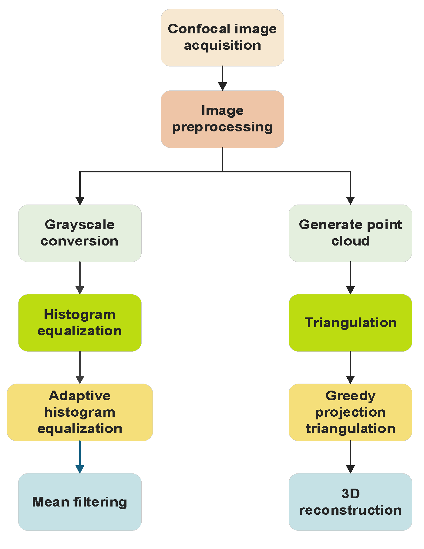
Figure 2.
Laser Scanning Confocal Microscope.
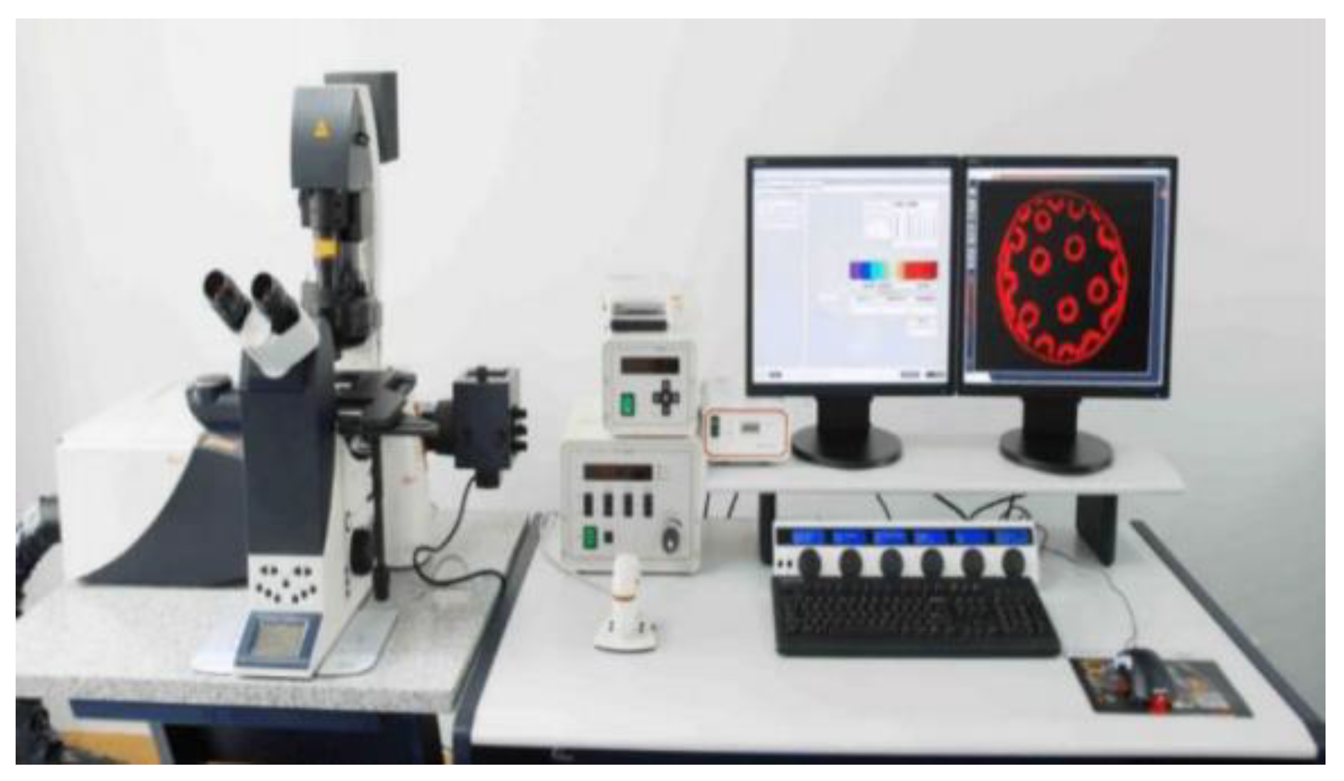
Figure 3.
Transmission image.
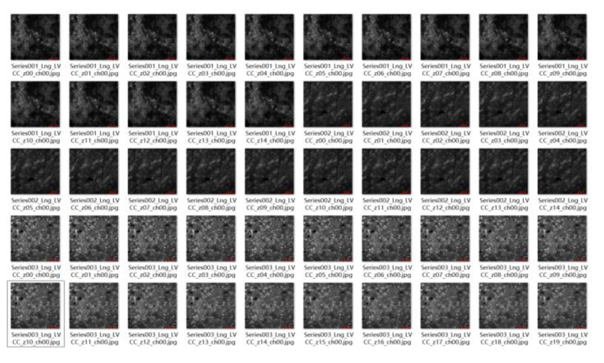
Figure 4.
light image.

Figure 5.
heavy image.
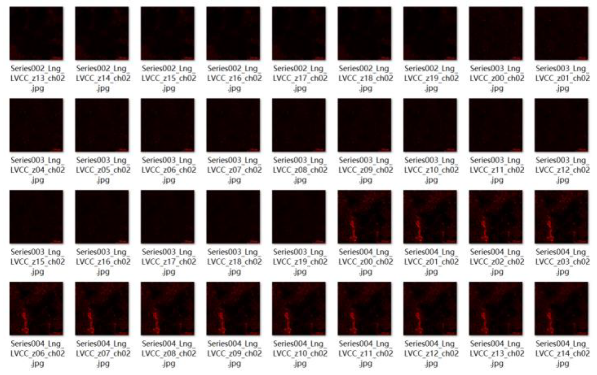
Figure 6.
Histogram of the source image.
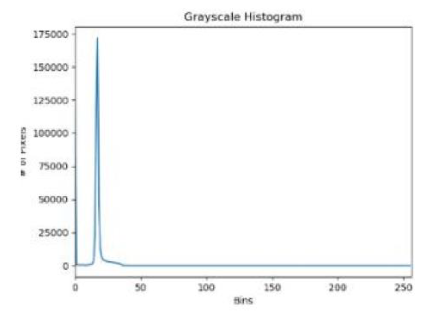
Figure 7.
Histogram after equalization processing.
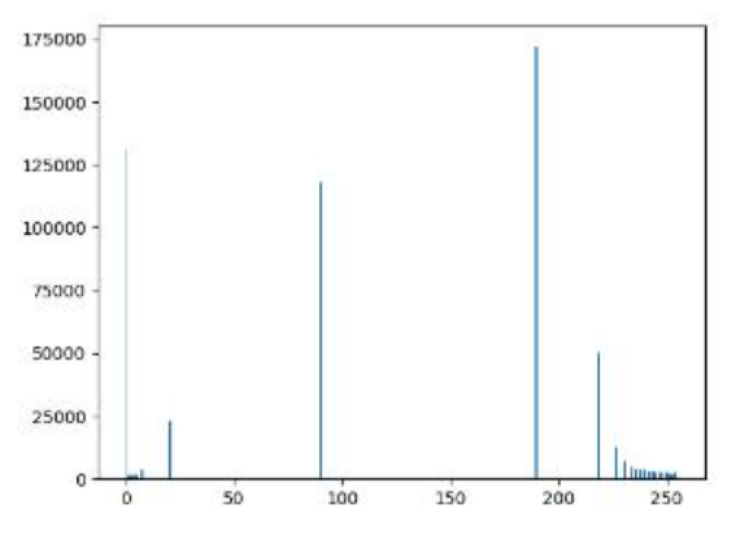
Figure 8.
Comparison between the source image and the image after equalization processing.
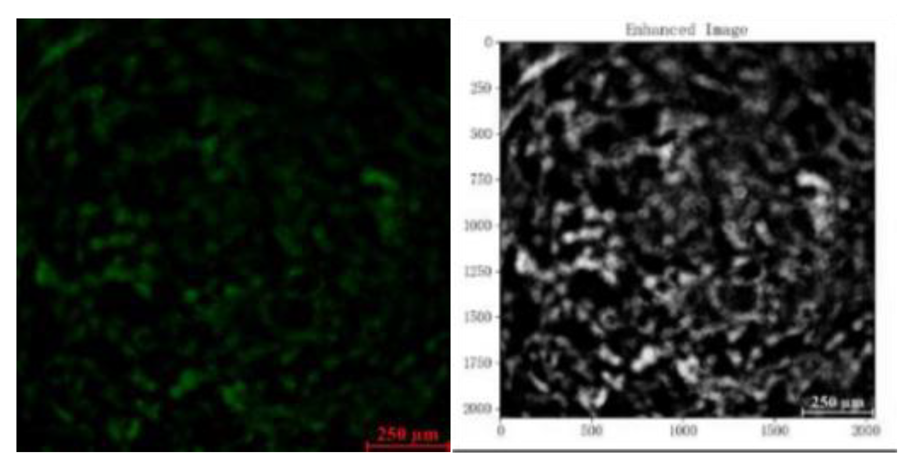
Figure 9.
Delaunay Triangulation Diagram.
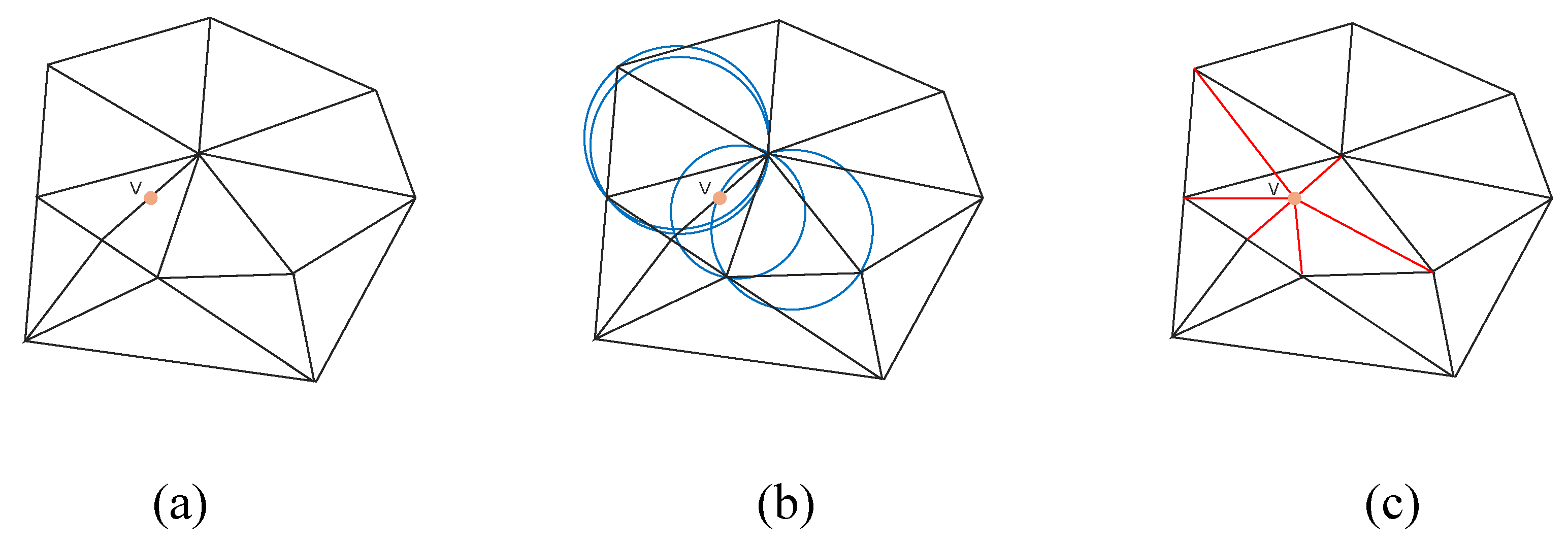
Figure 10.
Mesh Subdivision Diagram.
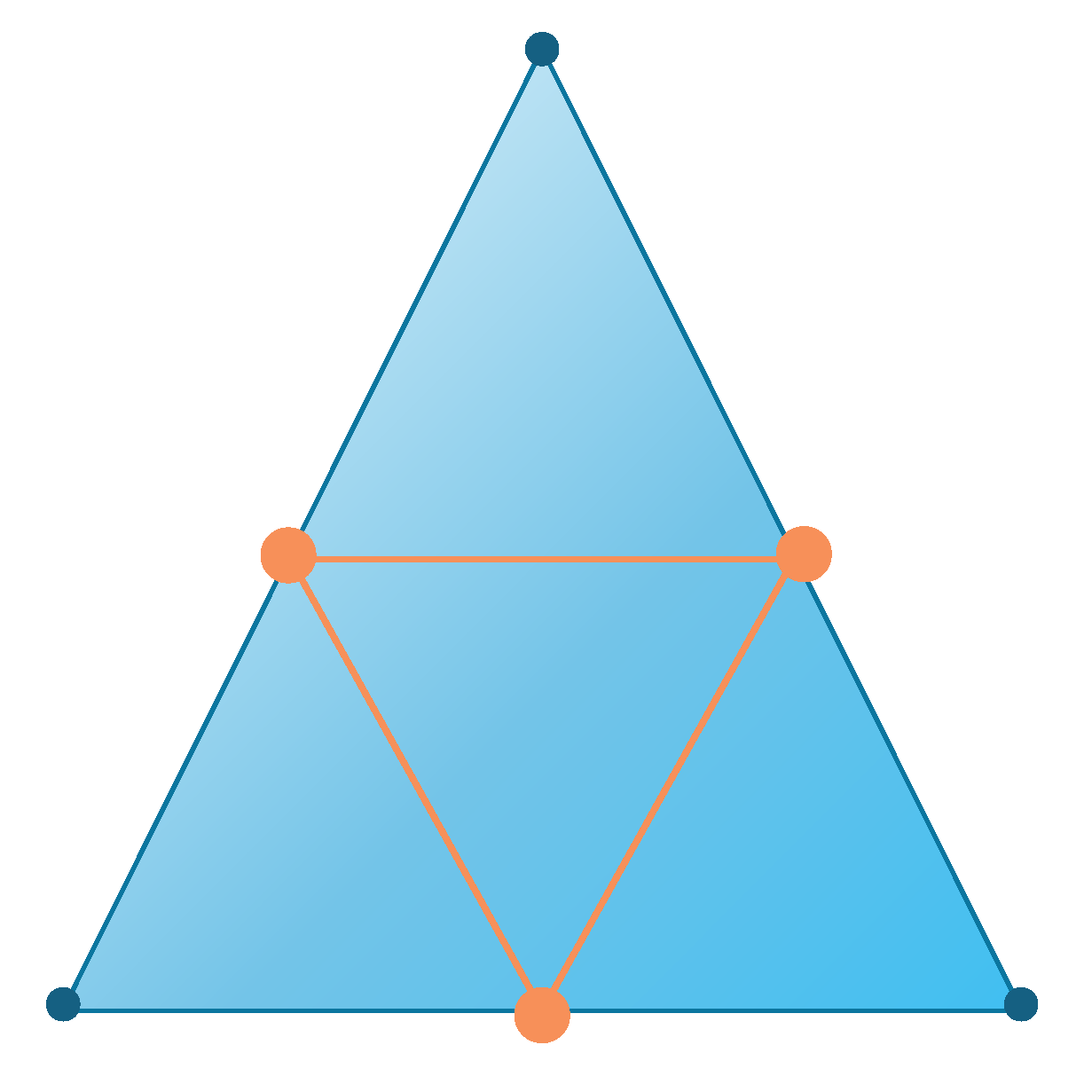
Figure 11.
Local Projection Diagram of k-Nearest Neighbors.
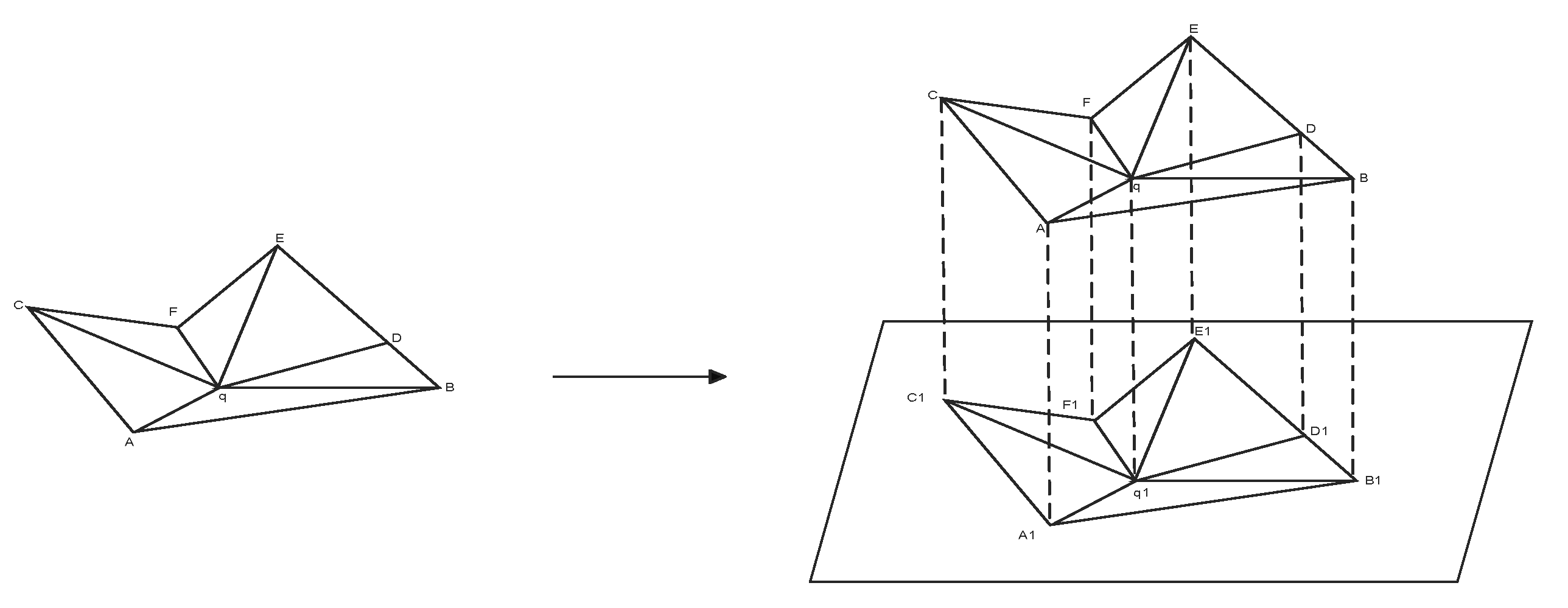
Figure 12.
Flowchart of Greedy Projection Triangulation.
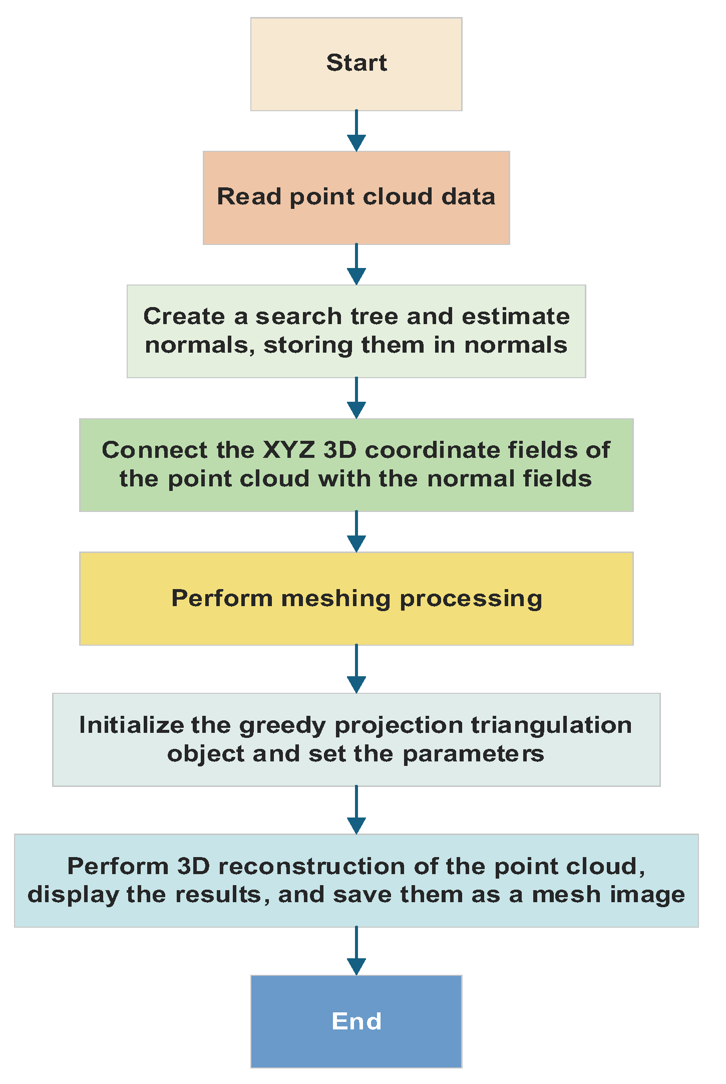
Figure 13.
3D Reconstruction Results from Different Perspectives.
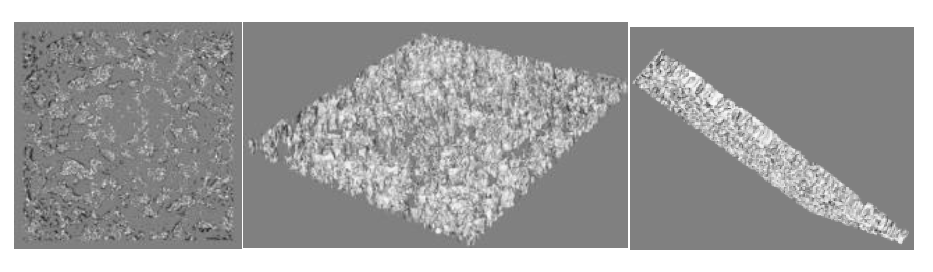
Figure 14.
Texture-Mapped 3D Reconstruction.
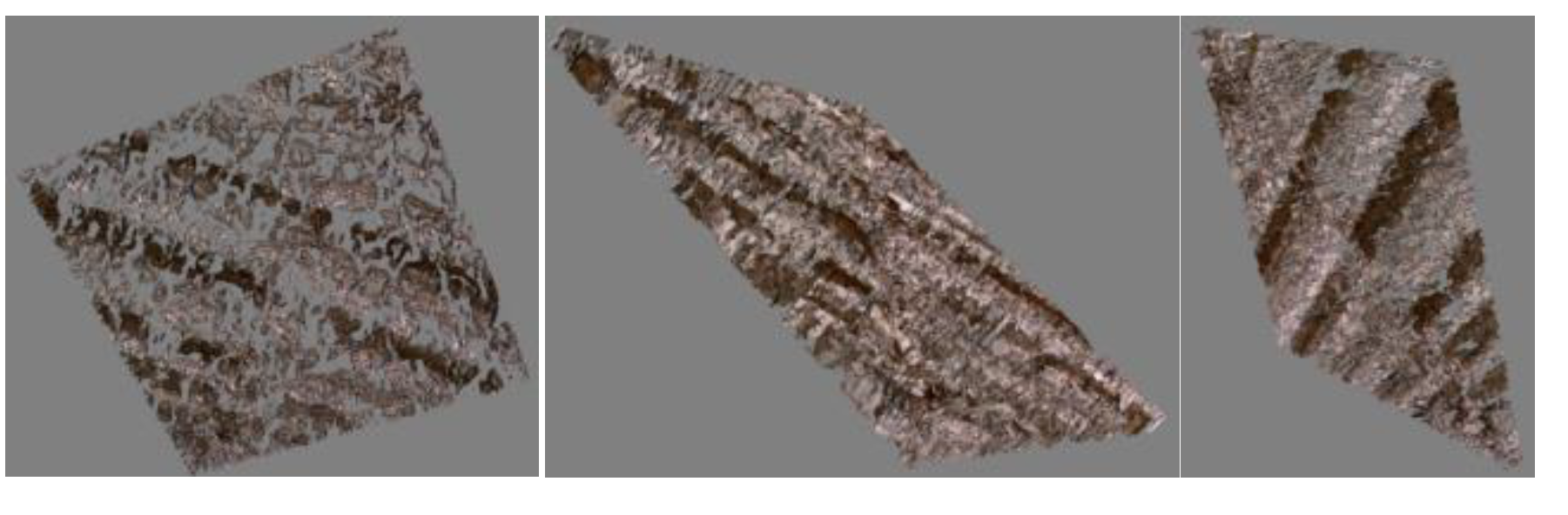

Table 1.
Laser Wavelength Range.
| Laser | Wavelength |
| 405 Diode | 405nm |
| Argon | 458nm,475nm,488nm,514nm |
| HeNe 543 | 543nm |
| DPS 561 | 561nm |
| HeNe 633 | 633nm |
Table 2.
Objective Lens Parameters.
| Magnification | Numerical Aperture |
| 10 | 0.3 |
| 20 | 0.5 |
| 40 | 0.85 |
Table 3.
Comparison of Two Mesh Optimization Methods.
| Feature | Laplacian Smoothing | Energy Minimization-Based Optimization |
| Implementation Complexity | Low | High |
| Computational Cost | Low | High |
| Applicability | Slightly irregular meshes | Meshes with complex or special requirements |
| Model Feature Preservation | Poor | Good |
| Detail Preservation | Poor | Good |
Table 4.
Three-dimensional modeling experiments based on confocal images.
| Evaluation Index | Average Value | Simple Region | Complex Region |
| Reconstruction Accuracy | 82% | 85% | 78% |
| Model Completeness | 75% | 80% | 70% |
| Processing Time (minutes) | 3 | 2.5 | 3.5 |
| Geometric Error (mm) | 0.05 | 0.05 | 0.1 |
Disclaimer/Publisher’s Note: The statements, opinions and data contained in all publications are solely those of the individual author(s) and contributor(s) and not of MDPI and/or the editor(s). MDPI and/or the editor(s) disclaim responsibility for any injury to people or property resulting from any ideas, methods, instructions or products referred to in the content. |
© 2025 by the authors. Licensee MDPI, Basel, Switzerland. This article is an open access article distributed under the terms and conditions of the Creative Commons Attribution (CC BY) license (http://creativecommons.org/licenses/by/4.0/).
Copyright: This open access article is published under a Creative Commons CC BY 4.0 license, which permit the free download, distribution, and reuse, provided that the author and preprint are cited in any reuse.


