Submitted:
23 April 2025
Posted:
23 April 2025
You are already at the latest version
Abstract
The paper investigates the deployment of data analytics and machine learning to improve welding quality in Tecnomulipast srl, a small-to-medium sized manufacturing firm located in Puglia, Italy. The firm produces food machine components and more recently mechanized its laser welding process with the introduction of an IoT-enabled system integrating photographic control. The investment, underwritten by the Apulia Region under PIA (Programmi Integrati di Agevolazione) allowed Tecnomulipast to not only mechanize its production line but also embark upon wider digital transformation. This involved the creation of internal data analytics infrastructures that have the capability to underpin machine learning and artificial intelligence applications. This paper addresses a prediction of weld bead width (LC) with a dataset of 1,000 observations. Input variables are laser power (PL), pulse time (DI), frequency (FI), beam diameter (DF), focal position (PF), travel speed (VE), trajectory accuracy (TR), laser angle (AN), gas flow (FG), gas purity (PG), ambient temperature (TE), and penetration depth (PE). The parameters were exploited to build and validate some supervised machine learning algorithms like Decision Trees, Random Forest, K-Nearest Neighbors, Support Vector Machines, Neural Networks, and Linear Regression. The performance of the models was measured by MSE, RMSE, MAE, MAPE, and R². Ensemble methods like Random Forest and Boosting performed the highest. Feature importance analysis determined that laser power, gas flow, and trajectory accuracy are the key variables. This project showcases the manner in which Tecnomulipast has benefited from public investment to introduce digital transformation and adopt data-driven strategies within Industry 4.0.
Keywords:
Tecnomulipast
; laser welding
; machine learning
; digital transformation
; Industry 4.0
1. Introduction
The increasing adoption of artificial intelligence and data analytics within production operations represents a paradigm shift for how production efficiency and quality are tracked and optimized. Although big industries have driven such developments, their application within small-to-medium enterprises (SMEs) of traditional industries like food machinery production is sparse and underresearched. This research bridges that gap by examining how a Southern Italian SME, Tecnomulipast srl, adopted a data-driven approach for predicting and controlling weld quality within an IoT-enabled laser welding machine. The main research question for this research is: To what extent can machine learning models effectively predict weld bead width (LC) as an essential quality metric from real-time process information observed from a digitally transformed welding machine? Despite the proliferation of sensor-rich production environments, extant research is of little help for SMEs that seek to effectively apply machine learning models for real-time quality prediction, especially for highly specialized processes such as laser welding. Most research tends to target big-industry implementation or is restricted within lab-scale experiments. This research offers a new case study of a regionally funded innovation project (via the Apulia Region’s PIA program) where a full-scale machine learning infrastructure was implemented and validated using 1,000 production samples. By comparing multiple supervised algorithms and selecting the best performing predictor, this research offers actionable findings into how SMEs can converge with Industry 4.0 values through extensive, interpretable, as well as scalable, data science techniques.
The article continues as follows, the second section presents the analysis of the literature, the third section presents the data and the variables, the fourth section contains the results of the machine learning regressions, the fifth section shows the results of the network analysis, the sixth section contains the conclusions.
2. Literature Review
The following commentary critically examines how recent research in the machine learning and laser welding fields supports and enlightens the Tecnomulipast srl, a small and medium-sized enterprise (SME) located within the region of Apulia, Southern Italy. Tecnomulipast is part of a digital transformation process, investing in the deployment of an automated laser welding system fed by an IoT solution and analytics infrastructure. The chosen articles are theoretically and practically relevant to the challenges and opportunities of the company as aligned with Industry 4.0 philosophies. The research by Wang et al. (2025) lays a solid groundwork by responding to issues of machine learning model generalizability in intelligent welding systems production within automotive production. Their concern for domain adaptation as well as transferability is of specific relevance for Tecnomulipast, an SME, as it, as many SMEs, will have to adapt advanced algorithms to its unique production process, frequently from less of both the necessary data as well as resources compared to large multinational companies. Their multi-sensor data utilization as well as their concern for robustness is closely aligned with the company’s approach of adopting an interconnected, sensor-intensive welding environment.
Ma et al. (2025) make a contribution by using an innovative hybrid strategy that integrates a Kolmogorov-Arnold Network (KAN) with a genetic algorithm for deep penetration laser welding optimization. Their two-layer approach is a balance between prediction accuracy and interpretability—two considerations fundamental for industrial environments where technicians need to trust as well as comprehend the judgments made by artificial intelligent systems. For Tecnomulipast, the use of interpretable models is essential given the low density of internal data science capabilities, as well as the necessity for actionable, transparent outputs from artificial intelligent systems.
The paper by Poornima et al. (2024) proposes a hybrid DNN-HEVA model for weld quality prediction of duplex stainless steel butt welds. Although specific to one material, the approach—merging deep learning with geometric analysis—is extensible to other applications, including Tecnomulipast production processes. Application of techniques for shape-aware modeling is of particular significance for their vision-based inspection system, given the prevalence of weld bead and joint geometrical information for quality evaluation. Din et al. (2024) break new ground for visual quality inspection by utilizing Vision Transformers for laser welding image classification. Their multi-model feature aggragation approach presents a direction for Tecnomulipast’s photographic process control, as it already samples images during welding processes. The attention mechanism of the transformer could prove crucial for enhancing defect identification, particularly for detecting subtle visual abnormalities that might be overlooked by standard CNNs.
In an applied context, Maculotti et al. (2024) provide a comparison of machine learning models for optimizing laser welding of deep-drawing steel. Their benchmarking strategy is directly applicable to Tecnomulipast’s project, wherein several supervised learning models (such as Random Forest, SVM, Neural Networks) were compared. The research highlights trade-offs between model interpretability, performance, and computational cost—considerations critical for SMEs balancing innovation with efficiency of operation. Hartung et al. (2023) provide a machine learning approach for weld geometric reconstruction as part of the overall vision for automation of quality control. Their research can be leveraged further for further development at Tecnomulipast, wherein inline inspection is envisioned as part of the digital transformation journey. Reconstructing weld geometry through sensor readings and regression models is a compelling option for minimizing reliance on human observation and enhancing consistency.
Ying-chao et al. (2023) concentrate on real-time monitoring through emission spectroscopy in laser wire welding. Since Tecnomulipast is not as of yet utilizing spectroscopic techniques, the essential principle—multiple-sensor, real-time weld pool monitoring—is very much relevant. Their research supports the necessity of multistreaming as a means of process control as well as detecting anomalies, consistent with Tecnomulipast’s IoT-capable arrangement. Chianese et al. (2022) examine the application of photodiodes for weld gap and penetration depth sensing of welding between copper and steel, especially for the welding of battery tabs. Their application of low-cost, high-frequency sensors could motivate cost-effective sensor integration by Tecnomulipast, most notably for real-time weld penetration sensing without the introduction of high-end vision systems.
Earlier, Cai et al. (2019) had shown how high-speed imaging and machine learning could be used for predicting weld bead width. Their findings confirmed the value of temporal imaging and algorithmic comparison, as exemplified by Tecnomulipast’s approach of using photographic information to predict quality factors such as bead width and penetration. Practical deployment of predictive models from image information is one of the key innovations of the Tecnomulipast project. Ozkat et al. (2017) and Sokolov et al. (2020) offer insights from the viewpoint of physics-based, as well as hybrid modeling. Ozkat’s multi-physics decoupling addresses variability caused by gaps between parts, while Sokolov’s research on keyhole mapping using optical coherence tomography underpins closed-loop control. Although such methods are complex and appropriate for higher-end manufacturing, they represent longer-term innovation pathways that Tecnomulipast could pursue as its system develops further and its digital infrastructure becomes established.
These articles demonstrate the international trend toward machine learning- and IoT-driven smart manufacturing systems. They endorse the notion that integrating data-driven models, interpretable artificial intelligence, real-time sensor input, and visual monitoring can make laser welding processes more adaptable and efficient. For Tecnomulipast srl, they provide both motivation and backing. This company, a small enterprise implementing digital transformation through support from its region of origin (PIA - Regione of Apulia, Italy), is a demonstration that even SMEs can be front-runners in implementing intelligent, data-driven technologies for optimizing production. By aligning its initiatives with the techniques and tenets examined within this advanced study, Tecnomulipast is an example for other small businesses within its region wishing to adopt Industry 4.0 technologies. The intersection of machine learning, autonomous inspection, and digital networking is not only a powerful tool for quality improvement, but for the larger sustainability and competitiveness of small manufacturers within the changing global industrial context (Table 1).
3. Data and Variables
The variables employed for training machine learning models for the prediction of production efficiency of a laser machine within a production firm consist of a mixture of process variables, environmental variables, and quality metrics. The product identifier (PRD2T) provides a distinct reference for each of the produced items, making it possible for them to be traced through the observations. Laser power (PL), pulse duration (DI), and pulse frequency (FI) determine the essential energy and temporal laser welding process specifications, which directly impact thermal input as well as welding stability. Beam diameter (DF) and focal position (PF) capture spatial accuracy as well as energy concentration on the target material, relevant for the stability of consistent weld penetration. The travel speed (VE) captures the speed of laser movement, impacting productivity as well as thermal diffusion. Trajectory and repeatability (TR) capture the mechanical accuracy of the machine, one of the most critical indicators of uniform weld paths as well as minimizing defects. The laser incident angle (AN) impacts energy absorption as well as weld geometry, of higher significance for reflective or complex materials. Gas flow (FG) and gas purity (PG) capture the weld pool shielding conditions, critical for preventing contamination as well as porosity. Ambient temperature (TE) captures context for thermal fluctuations that could affect stability of process. And finally, penetration depth (PE) as well as bead width (LC) are direct quality indicators of the weld as well as can be employed as target variables as well as efficiency as well as consistency proxies within supervised learning models that can predict the efficiency as well as uniformity of the laser machine (Table 2).
The information pertains to a company whose welding process is automated by a machine fitted with IoT as well as photographic inspection technologies. All variables have 1000 valid values with no missing values. Values seem normalized with z-score standardization, as evidenced by means near zero and standard deviations near one, making them ready for higher-level statistical analysis or machine learning applications. Both process parameters (laser power, pulse length, frequency, speed, beam width, focal position) as well as output characteristics (bead width, penetration) are the main variables. Their distributions have mild asymmetry and platykurtic behavior, with flatter distribution compared to a normal distribution. This is supported by consistently negative kurtosis values as well as by the Shapiro-Wilk test, whose p-values are lower than 0.001 for all variables, rejecting the normality hypothesis. The most relevant output variables, bead width (LC) and penetration (PE), have negative skewness, meaning that the data have heavier tails on the left side of the distribution and that welds most often have values higher than the mean, although by a minor amount. The machine would seem to have good operating stability, as interquartile ranges are thin, and median absolute deviations are low for all variables, meaning there is little dispersion. Since the non-normal distribution of the data, however, could make classical linear models insufficient for identifying underlying patterns, robust or non-parametric statistical analysis could be needed. Gas-related variables such as gas flow (FG) and gas purity (PG) have higher skewness and modes, perhaps as a consequence of batch variation, as well as of the application of different shielding strategies for different welding contexts. In summary, the data represent a technologically mature, well-maintained system, whose well-regulated parameters, however, have usual variation typical of industrial automation processes (Table 3).
4. Machine Learning
Assessing information on automatic welding within the framework of Industry 4.0 is a strategic action for a small-to-medium company such as Tecnomulipast srl, from Southern Italy operating within the food machinery production industry. IoT technology integration with real-time acquisition systems turns a standard production activity into an intelligent, trackable, and optimizable function. Data analysis from welding enables the company not only to track joint quality with accuracy, minimize process variation, predict anomalies, and enhance overall efficiency, but is critical for raising competitiveness within an industrialized, globalized world. Comparing between machine learning models such as Boosting, Decision Tree, K-Nearest Neighbors, Linear Regression, Neural Networks, Random Forest, Regularized Linear Regression, and Support Vector Machine is of prime relevance as each of the models differs as regards predictive capacity, interpretability, and adaptability to the dataset. Knowing the best-performing algorithm is not only a matter of selecting the best-performing solution, but the one that is stable, efficient, and scalable given available technical and infrastructural capabilities. Technically-scientifically, utilizing the following statistical indicators as evaluation metrics such as MSE (Mean Squared Error), MSE (scaled), RMSE (Root Mean Squared Error), MAE/MAD (Mean Absolute Error / Median Absolute Deviation), MAPE (Mean Absolute Percentage Error), R² (Coefficient of Determination) is methodologically accurate, widely adopted within the industrial data science best practices, and well-accepted within the scientific literature. These metrics enable an integral analysis of model quality by capturing error size (MSE, RMSE), outlier resistance (MAE, MAD), relative error (MAPE), as well as the capacity of the model for variance explanation of the target factor (R²). Their joint utilization enables a balanced, objective, reproducible evaluation that is best practice within industrial-grade data science.
We have estimated the following equation:
Facing the normalized performance measures of the various machine learning models used for the weld bead width (LC) prediction task, Random Forest is the most precision, stable, and generalization-capacity-rich algorithm. It consistently produces the best outcome for virtually all the evaluation metrics. In particular, it captures the lowest achievable values for MSE, MSE (scaled), RMSE, MAE/MAD, and MAPE—reflecting the smallest prediction error—while also capturing the highest value of R² (1.000) that guarantees perfect adaptability within the normalized framework. Boosting is likewise a highly performing algorithm, ranking second best by the majority of the metrics through an R² value of 0.806 as well as low error values for MSE (0.241), RMSE (0.174), and MAPE (0.116), reflecting high reliability as well as stability. Neural Networks exhibit competitive efficiency through an R² value of 0.758 coupled with relatively low values of MSE as well as MAPE, reflecting their suitability as an alternative. Support Vector Machines as well as Regularized Linear Regression prove mediocre efficiency, whereas K-Nearest Neighbors performs with the worst, through an R² value of 0.000 alongside the highest errors for all the metrics. The Decision Tree model performs better than KNN but not as efficiently as ensemble-based methods through its lower generalization capacity. To sum up, Random Forest is the best choice for the task through precision, stability, as well as generalization, whereas Boosting offers a strong alternative with equivalent reliability within predictive welding analytics (Table 4).
Selecting Random Forest as our best-performing model, we can analyze the feature importance values to see how much each of the input variables contributes toward predicting weld bead width (LC) most strongly. The table offers three indicators for each of the variables: Mean decrease in accuracy, Total increase in node purity, and Mean dropout loss. These all measure how much each of the variables contributes toward building the model’s predictability. By far the most powerful is clearly PE (penetration depth), with the highest mean decrease in accuracy (0.522), highest increase in node purity (94.680), and highest mean dropout loss (0.598). This is consistent with the expectation that weld penetration is closely correlated with bead width and is a very critical quality determinant of welding in the current scenario. Second is significantly PL (laser power) with a strong decrease in accuracy (0.369), a high node purity (68.918), and a very high dropout loss (0.399). Not unexpectedly, laser power directly controls the energy input during the welding process. Following are FG (gas flow) and PG (gas purity) with values for all metrics rather near-identical. Both of the parameters are crucial for providing a clean welding environment and for preventing defects, so their influence is not surprising. AN (laser angle) and DF (beam diameter) are moderately important, indicating a secondary but still contributary role toward the quality of the weld. Least of all are DI (pulse duration), VE (travel speed), and FI (pulse frequency). Their very low values for all metrics point toward a minor influence on the output within the specific operating window of this dataset. Least of all is TE (ambient temperature), PF (focal position), and TR (trajectory repeatability). These variables are most likely kept relatively constant during operation, or perhaps have previously had their optimal values optimized, so their variability is minimized, and their statistical impact is low. In conclusion, the Random Forest model singles out the penetration depth, laser power, and gas parameters as the prime drivers of bead width of weld during the automated process of Tecnomulipast srl. These findings not only make sense from the welding physics point of view, but they also offer actionable targets for controlling the process, as well as for optimizing the process, within the context of Industry 4.0 (Figure 1).
The following is an additive feature attribution output for five test cases, as given by the Random Forest model for predicting weld bead width (LC). The values, presumably created by a SHAP or equivalent interpretability procedure, demonstrate the contribution of each attribute, relative to a set value (the "Base" column, constant at –0.045 for all cases).
In both instances, the value predicted is much less than the base, varying between –1.226 and –1.390. This is a decrease from the base because of the cumulative adverse effects of some of the main features, specifically PE (penetration depth), PL (laser power), FG (gas flow), and PG (gas purity).
PE is consistently the greatest negative contributor in all cases, ranging from –0.38 to –0.384. This is consistent with what is observed in the feature importance as well: the greatest contribution is by penetration depth, significantly pulling the prediction down.
PL is seen to have strong negative effect, from –0.287 to –0.296. This is consistent with its function of regulating power input—greater power can result in wider bead width, and such deviations from optimal power values would contribute negatively within these given test cases.
FG and PG have strong to moderate negative effects, supporting the significance of gas parameters for weld quality. The steady values for all the cases (approximately between –0.17 and –0.20 for FG, and between –0.13 and –0.15 for PG) demonstrate stable, though considerable, impact on the estimated outcome.
The other variables, such as DF (beam diameter) and AN (angle of incidence), have negative contributions across all instances, though less so. Their directional regularity assures constant though secondary impacts on the model's projections.
In contrast, variables such as VE (speed of travel) and PF (position of focus) display slight positive or zero effects, occasionally helping raise the prediction by a slight amount. FI (pulse frequency), DI (pulse duration), TR (repeatability of trajectory), and TE (ambient temperature) have near-zero or low effects, consistent with their low values of feature importance. In conclusion, such findings uphold interpretability and internal consistency of the Random Forest model. The most salient features—penetration depth, laser power, and gas flow settings—exhibit the highest and most uniform effects on the predictions for varying test cases. This reflects the model’s capability for yielding trustworthy, understandable information for quality control of welding for applications such as real-time predictive systems within the context of Industry 4.0 (Figure 2).
5. Network Analysis
After performing a machine learning analysis, it is logical, therefore, to apply network analysis with centrality metrics because machine learning models are good at predicting but do not necessarily capture the internal dynamics of interdependencies among variables. Network analysis offers a structural representation of the relationships, giving further insight into the interplay of variables with each other within the system. By examining centrality metrics like betweenness, closeness, strength, and expected influence, one can determine where variables are central, where they are bridges, and where they are on the periphery. For example, PL (laser power) is ranked highest for all centrality metrics, meaning that it is the most powerful, influencing role within the network of variables. This is as expected given its probable significance within predictive models. DF (beam diameter) and PF (focal position) have significant betweenness, meaning they are connectors between variables, potentially affecting multiple paths even though they are not necessarily the most direct influencers. In contrast, for variables such as DI, FI, and TR, there are negative values for all metrics, suggesting they are not so much central and potentially have isolated effects on the system. Furthermore, network analysis offers the ability to corroborate the machine learning by comparing network metrics with importances from the model, as well as identifying redundant, weakly connected variables, facilitating reduction of dimensions and feature choice. Having the ability to see possible chains of influence among variables improves interpretability of intricate models, such as within industrial environments where behavior of the system is as critical as is predictive accuracy. In all, the combination of network analysis with centrality metrics following machine learning creates a fuller, system-level view that helps interpret models, streamline processes, as well as make informed choices on variable significance as well as role interplay (Figure 3).
6. Conclusions
The paper showcases the real-world application value of IoT-enabled data acquisition systems coupled with machine learning methods for improving weld quality prediction for a small-to-medium-sized manufacturing company. In a real-case study of Tecnomulipast srl based in Gravina in Puglia, supported by public funds through the PIA program, the research showcases how a digitalized production environment can make sophisticated predictive analytics available for laser welding. Among the machine learning algorithms applied, Random Forest was identified as the best-performing algorithm, indicating the best prediction accuracy for all the considered performances (MSE, RMSE, MAE, MAPE, and R²). The chosen model not only produced low prediction errors, but for detailed interpretability, feature significance analysis as well as additive contribution methods could be employed. Penetration depth (PE), laser power (PL), and gas flow parameters (FG, PG) were recognized as the main factors affecting weld bead width (LC), yielding actionable insights for process improvement as well as quality control.
In addition, the application of network analysis based on centrality indicators provided a complementary view of interdependencies among variables. This methodology disclosed structural interconnections between parameters, corroborating machine learning evidence and allowing for better interpretability of models. Laser power and beam geometry turned out to be central variables within the topology of the system, indicating their decisive impact not only on output quality but on process dynamics as well. Altogether, the research affirms that a union of machine learning with network analysis yields predictive capabilities, as well as systemic insight. For SMEs, looking forward to adapting to Industry 4.0, this dual strategy addresses a scalable, transparent, and efficient framework for optimizing production through data.
Acknowledgement
Results obtained in the research and development project "Tecnomulipast" - Codice Pratica 683TK4 - a valere sul Bando Programmi Integrati di Agevolazioni PIA Piccole Imprese (Art 27 Reg. Regionale 17/2014 e smi).
References
- Wang, P. E., Ghassemi-Armaki, H., Pour, M., Zhao, X., Ma, J., Sattari, K., & Carlson, B. (2025). Applicable and generalizable machine learning for intelligent welding in automotive manufacturing. Welding in the World, 1-36. [CrossRef]
- Ma, S., Leng, J., Chen, Z., Du, Y., Zhang, X., & Liu, Q. (2025). Intrinsically and Post-Hoc Interpretable Kolmogorov-Arnold Network and Genetic Algorithm for Laser Deep Penetration Welding Parameters Optimization. IEEE Transactions on Instrumentation and Measurement. [CrossRef]
- Poornima, C. L., Rao, C. S., & Varma, D. N. (2024). Predicting weld quality in duplex stainless steel butt joints during laser beam welding: a hybrid DNN-HEVA approach. Journal of Advanced Manufacturing Systems, 23(04), 801-836. [CrossRef]
- Din, N. U., Zhang, L., Nawaz, M. S., & Yang, Y. (2024). Multi-model feature aggregation for classification of laser welding images with vision transformer. Journal of King Saud University-Computer and Information Sciences, 36(5), 102049. [CrossRef]
- Maculotti, G., Genta, G., & Galetto, M. (2024). Optimisation of laser welding of deep drawing steel for automotive applications by Machine Learning: A comparison of different techniques. Quality and Reliability Engineering International, 40(1), 202-219. [CrossRef]
- Hartung, J., Jahn, A., & Heizmann, M. (2023). Machine learning based geometry reconstruction for quality control of laser welding processes. tm-Technisches Messen, 90(7-8), 512-521. [CrossRef]
- Ying-chao, F., Yi-ming, H., Jin-ping, L., Chen-peng, J., Peng, C., Shao-jie, W., ... & Huan-wei, Y. (2023). On-Line Monitoring of Laser Wire Filling Welding Process Based on Emission Spectrum. SPECTROSCOPY AND SPECTRAL ANALYSIS, 43(6), 1927-1935.
- Chianese, G., Franciosa, P., Nolte, J., Ceglarek, D., & Patalano, S. (2022). Characterization of photodiodes for detection of variations in part-to-part gap and weld penetration depth during remote laser welding of copper-to-steel battery tab connectors. Journal of Manufacturing Science and Engineering, 144(7), 071004. [CrossRef]
- Cai, W., Wang, J., Cao, L., Mi, G., Shu, L., Zhou, Q., & Jiang, P. (2019). Predicting the weld width from high-speed successive images of the weld zone using different machine learning algorithms during laser welding. Math. Biosci. Eng, 16(5), 5595-5612. [CrossRef]
- Ozkat, E. C., Franciosa, P., & Ceglarek, D. (2017). Development of decoupled multi-physics simulation for laser lap welding considering part-to-part gap. Journal of Laser Applications, 29(2). [CrossRef]
- Sokolov, M., Franciosa, P., Al Botros, R., & Ceglarek, D. (2020). Keyhole mapping to enable closed-loop weld penetration depth control for remote laser welding of aluminum components using optical coherence tomography. Journal of Laser Applications, 32(3). [CrossRef]
Figure 1.
Feature Importance Metrics of Random Forest Regression. .
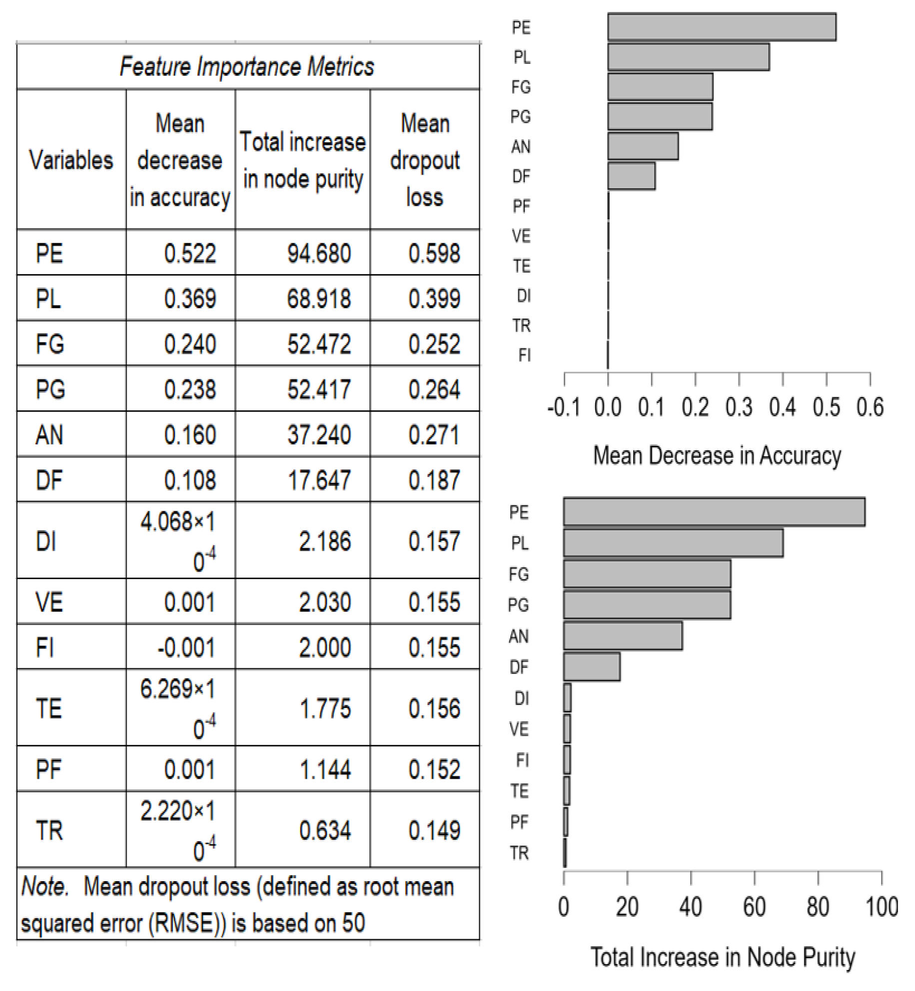
Figure 2.
Predictions using Random Forest Regression.
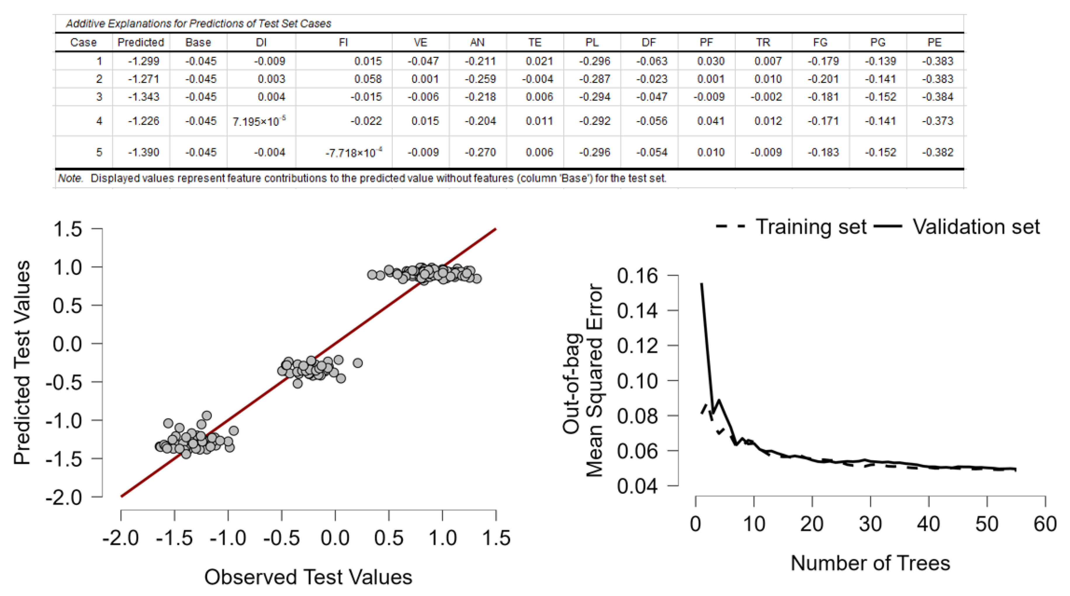
Figure 3.
Network Analysis.
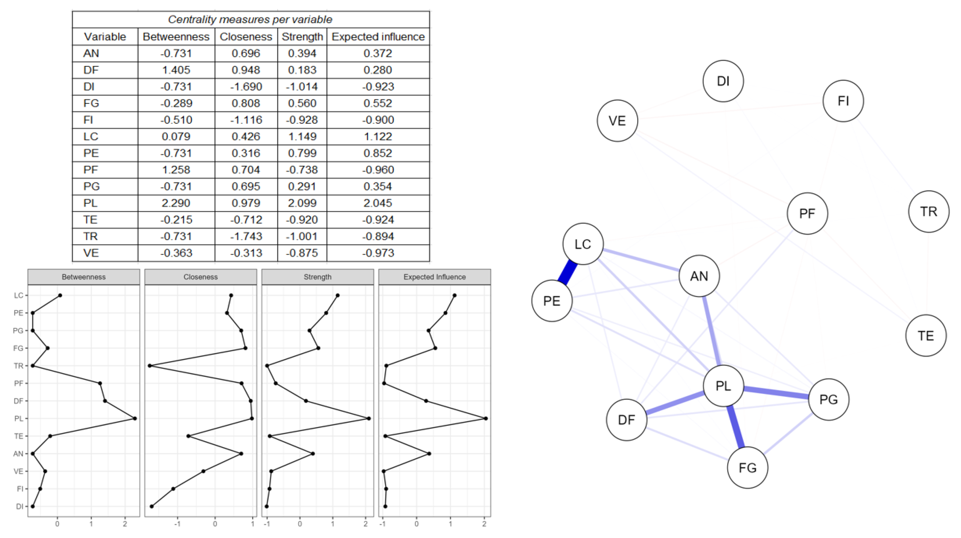

Table 1.
Synthesis of the literature.
| Macro-theme | Reference | Key Contribution | Relevance to Tecnomulipast |
|---|---|---|---|
| Generalizable & Scalable ML for Welding | Wang et al. (2025) | Generalizable ML framework for intelligent welding in automotive contexts | Supports the transfer of scalable ML models to SME-level environments like Tecnomulipast’s real-world setup |
| Maculotti et al. (2024) | Comparison of ML algorithms for laser welding optimization | Helps choose the most efficient and interpretable algorithm given SME constraints and real production data | |
| Interpretable & Hybrid AI Models | Ma et al. (2025) | Interpretable Kolmogorov-Arnold Network with genetic optimization | Offers a transparent model for parameter tuning, suitable for a resource-limited SME |
| Poornima et al. (2024) | Hybrid DNN-HEVA model for weld quality prediction | Shows the benefit of combining geometry-aware models with AI, useful in Tecnomulipast’s photo-based inspections | |
| Image-Based Monitoring & Vision AI | Din et al. (2024) | Vision Transformer with feature aggregation for weld image classification | Directly relevant to Tecnomulipast’s photographic system for monitoring welds in real time |
| Cai et al. (2019) | Prediction of weld bead width from high-speed images using various ML algorithms | Validates the image-based predictive approach used by Tecnomulipast | |
| Inline Quality Control & Process Monitoring | Hartung et al. (2023) | Geometry reconstruction using ML for automated weld quality control | Useful for extending Tecnomulipast’s inspection system with automated defect detection |
| Ying-chao et al. (2023) | Real-time monitoring via emission spectra in laser wire welding | Reinforces the importance of continuous monitoring, even if different sensing tech is used | |
| Chianese et al. (2022) | Photodiode-based gap and penetration monitoring in dissimilar metal welding | Suggests low-cost sensor strategies for penetration monitoring applicable to SMEs | |
| Process Control & Closed-Loop Systems | Sokolov et al. (2020) | Optical coherence tomography for closed-loop penetration control | Presents a future direction for Tecnomulipast’s system evolution towards real-time adaptive control |
| Ozkat et al. (2017) | Multi-physics simulation accounting for part-to-part gap in laser welding | Supports hybrid modeling to complement ML, useful for better understanding material-behavior interaction |
Table 2.
Description of Variables.
| Description | Unit of measurement and range | Acronym | |
| Product | Unique identifier for each product produced. | It is represented with a progressive number. | PRD2T |
| Laser power (W) | Energy supplied by the laser to perform the welding. | Expressed in Watts (W). Usually variable between 1500 W and 1800 W. | PL |
| Pulse duration (ms) | Time during which the laser remains active for each pulse. | Expressed in milliseconds (ms). Variable between 5 and 8 ms. | DI |
| Pulse frequency (Hz) | Number of laser pulses per second. | Expressed in Hertz (Hz). Typically variable between 2000 and 2300 Hz. | FI |
| Beam diameter (µm) | Width of the laser beam at the welding point. | Expressed in microns (µm). Typically between 100 and 130 µm. | DF |
| Focal position (mm) | Focal distance from the material surface. | Expressed in millimeters (mm). Varies between -0.5 mm, 0 mm, +0.5 mm, 1 mm. | PF |
| Travel speed (mm/s) | Speed with which the laser moves during the welding process. | Expressed in mm/s. Varies between 10 and 13 mm/s. | VE |
| Trajectory and repeatability | Accuracy and repeatability of the laser movement system. | Typical values: < ±0.1 mm, < ±0.15 mm, < ±0.2 mm, < ±0.25 mm. | TR |
| Laser incidence angle (°) | Angle formed by the laser beam from the material surface. | Typical values: 75°, 80°, 85°, 90°. | AN |
| Gas flow | Type of gas used to protect the welding pool and keep it pure. | Expressed in l/min for flow | FG |
| Gas purity | Type of gas used to protect the welding pool and keep it pure. | % for purity. | PG |
| Ambient temperature (°C) | Temperature of the environment in which the welding is performed. | Variable between 25°C and 28°C. | TE |
| Penetration (mm) | Depth of the welding in the material. | Expressed in mm. Typically between 1.5 mm and 3.5 mm. | PE |
| Bead width (µm) | Width of the welding line generated by the laser. | Expressed in microns (µm). Typically between 200 µm and 500 µm. | LC |
Table 3.
Descriptive Statistics.
| LC | DI | FI | VE | AN | TE | PL | DF | PF | TR | FG | PG | PE | |
| Valid | 1000 | 1000 | 1000 | 1000 | 1000 | 1000 | 1000 | 1000 | 1000 | 1000 | 1000 | 1000 | 1000 |
| Missing | 0 | 0 | 0 | 0 | 0 | 0 | 0 | 0 | 0 | 0 | 0 | 0 | 0 |
| Mode | 0.731 | 0.610 | -1.607 | 0.283 | -1.315 | 1.343 | 1.164 | -0.839 | 1.145 | 1.096 | -1.646 | 1.192 | -1.326 |
| Median | 0.277 | 0.011 | -0.039 | 0.014 | -0.010 | -0.010 | 0.057 | -0.024 | 0.278 | 0.190 | -0.099 | 0.318 | 0.267 |
| Mean | -7.000×10⁻⁹ | 1.000×10⁻⁹ | 1.400×10⁻⁸ | 3.000×10⁻⁹ | 5.000×10⁻⁹ | -2.100×10⁻⁸ | 2.600×10⁻⁸ | 6.000×10⁻⁹ | 1.050×10⁻⁷ | 7.800×10⁻⁸ | -3.189×10⁻¹⁸ | 3.900×10⁻⁸ | 6.000×10⁻⁹ |
| Std. Deviation | 1.001 | 1.001 | 1.001 | 1.001 | 1.001 | 1.001 | 1.001 | 1.001 | 1.001 | 1.001 | 1.001 | 1.001 | 1.001 |
| Coefficient of variation | -1.429×10+8 | 1.001×10+9 | 7.146×10+7 | 3.335×10+8 | 2.001×10+8 | -4.764×10+7 | 3.848×10+7 | 1.668×10+8 | 9.529×10+6 | 1.283×10+7 | -3.138×10+17 | 2.565×10+7 | 1.668×10+8 |
| MAD | 0.686 | 0.876 | 0.871 | 0.841 | 0.967 | 0.861 | 1.010 | 0.863 | 0.867 | 0.905 | 0.927 | 0.829 | 0.734 |
| MAD robust | 1.017 | 1.298 | 1.291 | 1.247 | 1.434 | 1.277 | 1.498 | 1.280 | 1.286 | 1.342 | 1.375 | 1.229 | 1.089 |
| IQR | 2.068 | 1.751 | 1.758 | 1.683 | 1.934 | 1.699 | 2.008 | 1.728 | 2.169 | 2.112 | 1.855 | 1.883 | 1.995 |
| Variance | 1.001 | 1.001 | 1.001 | 1.001 | 1.001 | 1.001 | 1.001 | 1.001 | 1.001 | 1.001 | 1.001 | 1.001 | 1.001 |
| Skewness | -0.380 | 0.003 | 0.076 | 0.011 | 0.019 | -0.033 | 0.001 | 9.900×10⁻⁴ | -0.211 | -0.148 | 0.001 | -0.280 | -0.353 |
| Std. Error of Skewness | 0.077 | 0.077 | 0.077 | 0.077 | 0.077 | 0.077 | 0.077 | 0.077 | 0.077 | 0.077 | 0.077 | 0.077 | 0.077 |
| Kurtosis | -1.473 | -1.221 | -1.188 | -1.170 | -1.510 | -1.198 | -1.931 | -1.222 | -1.473 | -1.651 | -1.580 | -1.471 | -1.392 |
| Std. Error of Kurtosis | 0.155 | 0.155 | 0.155 | 0.155 | 0.155 | 0.155 | 0.155 | 0.155 | 0.155 | 0.155 | 0.155 | 0.155 | 0.155 |
| Shapiro-Wilk | 0.856 | 0.953 | 0.953 | 0.957 | 0.913 | 0.954 | 0.749 | 0.954 | 0.854 | 0.811 | 0.895 | 0.880 | 0.894 |
| P-value of Shapiro-Wilk | < .001 | < .001 | < .001 | < .001 | < .001 | < .001 | < .001 | < .001 | < .001 | < .001 | < .001 | < .001 | < .001 |
| Range | 3.173 | 3.456 | 3.426 | 3.494 | 3.675 | 3.482 | 2.330 | 4.474 | 2.602 | 2.414 | 3.431 | 3.514 | 3.734 |
| Minimum | -1.838 | -1.717 | -1.687 | -1.739 | -1.886 | -1.755 | -1.166 | -2.257 | -1.457 | -1.318 | -1.646 | -2.322 | -2.085 |
| Maximum | 1.335 | 1.739 | 1.739 | 1.755 | 1.789 | 1.727 | 1.164 | 2.216 | 1.145 | 1.096 | 1.786 | 1.192 | 1.649 |
| 25th percentile | -1.169 | -0.876 | -0.884 | -0.850 | -0.964 | -0.825 | -1.004 | -0.875 | -1.024 | -1.017 | -0.925 | -0.936 | -1.105 |
| 50th percentile | 0.277 | 0.011 | -0.039 | 0.014 | -0.010 | -0.010 | 0.057 | -0.024 | 0.278 | 0.190 | -0.099 | 0.318 | 0.267 |
| 75th percentile | 0.899 | 0.875 | 0.874 | 0.832 | 0.970 | 0.874 | 1.004 | 0.853 | 1.145 | 1.096 | 0.930 | 0.947 | 0.889 |
| Sum | -7.000×10⁻⁶ | 1.000×10⁻⁶ | 1.400×10⁻⁵ | 3.000×10⁻⁶ | 5.000×10⁻⁶ | -2.100×10⁻⁵ | 2.600×10⁻⁵ | 6.000×10⁻⁶ | 1.050×10⁻⁴ | 7.800×10⁻⁵ | -1.665×10⁻¹⁵ | 3.900×10⁻⁵ | 6.000×10⁻⁶ |
Table 4.
Machine learning analysis results with an indication of the performance of the algorithms.
| Metric | Boosting | Decision Tree | KNN | Linear Regression | Neural Net | Random Forest | Regularized Linear | SVM |
| MSE | 0.241 | 0.379 | 1.000 | 0.655 | 0.310 | 0.000 | 0.586 | 0.517 |
| MSE (scaled) | 0.179 | 0.393 | 1.000 | 0.393 | 0.250 | 0.000 | 0.536 | 0.464 |
| RMSE | 0.174 | 0.297 | 1.000 | 0.487 | 0.165 | 0.000 | 0.408 | 0.382 |
| MAE / MAD | 0.051 | 0.000 | 1.000 | 0.759 | 0.228 | 0.088 | 0.684 | 0.620 |
| MAPE | 0.116 | 0.000 | 1.000 | 0.312 | 0.165 | 0.005 | 0.803 | 0.115 |
| R² | 0.806 | 0.645 | 0.000 | 0.516 | 0.758 | 1.000 | 0.452 | 0.581 |
Disclaimer/Publisher’s Note: The statements, opinions and data contained in all publications are solely those of the individual author(s) and contributor(s) and not of MDPI and/or the editor(s). MDPI and/or the editor(s) disclaim responsibility for any injury to people or property resulting from any ideas, methods, instructions or products referred to in the content. |
© 2025 by the authors. Licensee MDPI, Basel, Switzerland. This article is an open access article distributed under the terms and conditions of the Creative Commons Attribution (CC BY) license (http://creativecommons.org/licenses/by/4.0/).
Copyright: This open access article is published under a Creative Commons CC BY 4.0 license, which permit the free download, distribution, and reuse, provided that the author and preprint are cited in any reuse.


